Minimization of Machine Speed Deviation by
Eigenvalue Adjusment of State Matrix of
Interconnected Network Fitted with UPFC and
Power Oscillation Damper
Dr I. I. Alabi, Dr A. I. Araga, F.O. Adunola
Department Of Electrical/Electronic Engineering, Nigerian Defence Academy,Kaduna, Nigeria.
ABSTRACT: In this paper the approach of eigenvalue adjustment of state matrix of a large interconnected network is used to minimize the machine speed deviations for a large interconnected Network fitted with FACTS device and Power Oscillation Damper. As a foundational work the generalized mathematic model of multi-machine power system with embedded FACTS was developed. This is principally aimed at providing benchmark models to enable in-depth analysis of dynamic and transient performances of the Machines when subjected to credible disturbance scenarios at different operating points. The results obtained clearly reveals the effectiveness of this approach
Keywords: UPFC, POD, Damping, Speed Deviation
I. INTRODUCTION
Wide variations in consumer demands often lead to perturbations in the power system dynamics. Whenever there is an imbalance between the mechanical input power to the rotor and the electrical output power from the stator electromechanical oscillation is triggered in the generator, the power transmission network consists of transmission lines, transformers and other energy storing accessories through which the ripples of this energy imbalance is transmitted as oscillation across the whole network. These oscillations are sometimes prolonged low frequency types that can lead to adverse effects on the performance of the power system in general and in extreme cases, culminate in catastrophic system failure. This research intends to deploy eigenvalue analysis method to a network embedded with FACTS Device and Power Oscillation Damper for the purpose of damping these oscillations and maintain the performance of an integrated power system at optimal level.
II. LITERATURE REVIEW
Eigenvalue analysis (modal analysis) is a valuable tool in analysis of power system small signal stability. It provides information about the inherent dynamic characteristic of the power system and assists in its design. It is typically used in studies of inter-area oscillations [1]. Eigenvalues can be used to determine the small-signal stability of the power systems. They are also good indicators for the bifurcation points such as saddle-node bifurcation and Hopf bifurcation. Eigenvalues and eigenvectors can be used to determine mode shapes, participation factors, controllability and observability of each mode.
Eigenvalues with the largest real parts and eigenvalues with the least damping ratios are of great importance for power system applications. In power system analysis, eigenvalues are widely used to study system uncertainty, estimate stability boundary, and enhance system stability performance. Eigenvalue computation is a linear analysis technique based on the linearized model. In reference [2], the author summarize the main research developments in the computational methods for eigenvalue problems during the 20th century.
eigenvalue computation algorithms, the Arnoldi method is believed to be the most efficient approach. But the method is heavily influenced by the selection of the number of guard vectors. The only way to explore this is by numerical tests.
It has been assumed that the dominant eigenvalue is the critical eigenvalue that will eventually cross the imaginary axis [6], but this may not always be the
case especially when the current operating point is some distance away from the instability boundary.
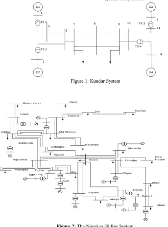
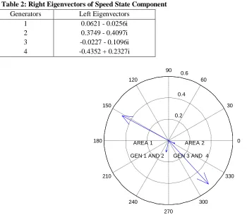
III. DESCRIPTION OF TEST SYSTEM Figures 1 and 2 shows the single line diagram of the test systems used. Details of system data are given in [7-8]. The sub-transient models of the systems synchronous machines were used with the detailed dynamic model of other embedded system components.
G1
G2
G3
G4 1
5
2
6
7 9 10
3
11
4 8
TX 1 TX 3
TX 4 TX 2
Figure 1: Kundur System
M4 Shiroro Kaduna
Kano
Gombe Kainji
Birnin Kebbi
Jebba GS Jebba
Oshogbo
Aiyede
Egbin
Egbin PS Akangba
AES
Ikeja West Benin
Ajaokuta
Onitsha
New Haven
Okpai Aja
Sapele
Aladja
Delta1
Delta 2
Afam Alaoji Jos
Katampe
IV. PROPOSED APPROACH
An electric power system can be represented by a set of non-linear differential-algebraic equations (DAE), as follows [9]
𝑥 = 𝑓 𝑥, 𝑦, 𝑢
0 = 𝑔 𝑥, 𝑦, 𝑢 (1) 𝑤 = 𝑥, 𝑦, 𝑢
After solving the power flow problem, a modal analysis is carried out by computing the eigenvalues and the participation factors of the state matrix of the system [2]. Linearizing equation (1) at an equilibrium point yields equation (2)
∆𝑥 0 ∆𝑤
=
𝐹𝑥 𝐹𝑦 𝐹𝑢
𝐺𝑥 𝐺𝑦 𝐺𝑢
𝐻𝑥 𝐻𝑦 𝐻𝑢
∆𝑥∆𝑦 ∆𝑢
(2)
𝐹𝑥= ∇𝑥𝐹𝑓 , 𝐹𝑦 = ∇𝑦𝐹𝑓, 𝐹𝑢 = ∇𝑢𝐹𝑓, 𝐺𝑥= ∇𝑥𝐺𝑔, 𝐺𝑦 = ∇𝑦𝐺𝑔, 𝐺𝑢 = ∇𝑢𝐺𝑔,𝐻𝑥= ∇𝑥𝐻, 𝐻𝑦= ∇𝑦𝐻,
𝐻𝑢 = ∇𝑢𝐻
Eliminating ∆𝑦 , and assuming that power flow Jacobian 𝐺𝑦 is non-singular (i.e. the system does
not show a singularity induced bifurcation), the state matrix A ( 𝐴 ∈ ℛ𝑛𝑥𝑛 ) of the system is given by 𝐴 = 𝐹𝑥− 𝐹𝑦𝐺𝑦−1𝐺𝑥 and the state space representation of equation (2) is
∆𝑥 = 𝐴∆𝑥 + 𝐵∆𝑢 (3) ∆𝑤 = 𝐶∆𝑥 + 𝐷∆𝑢
where the input matrix 𝐵 = 𝐹𝑢− 𝐹𝑦𝐺𝑦−1𝐺𝑢 (𝐵 ∈ ℛ𝑛𝑥𝑟), the output matrix 𝐶 = 𝐻𝑥− 𝐻𝑦𝐺𝑦−1𝐺𝑥
(𝐶 ∈ ℛ𝑚𝑥𝑛), and the feed forward matrix 𝐷 = 𝐹𝑢− 𝐻𝑦𝐺𝑦−1𝐺𝑢 (𝐷 ∈ ℛ𝑚𝑥𝑟).The state-space representation is the
base for controller design [10].
𝑥 ∈ ℛ𝑛 , is the vector of the state variables
𝑢 ∈ ℛ𝑙 is a set of controllable parameters (e.g controller reference signal)
𝑦 ∈ ℛ𝑚 is the vector of algebraic variables (e.g., bus voltage magnitudes and phase angles);
𝑤 ∈ ℛ𝑘 is a set of output variables (e.g., line current flows);
f is a set of differential equations that represents system and controller dynamics:
(𝑓: ℛ𝑛. ℛ𝑚. ℛ𝑙 → ℛ𝑛)
g is a set of algebraic equations that represents the transmission network power flows (𝑔: ℛ𝑛. ℛ𝑚. ℛ𝑙→ ℛ𝑚) h is a set of equations that represents output variables (e.g., measurements), such as line power flows and rotor angle speeds. (: ℛ𝑛. ℛ𝑚. ℛ𝑙 → ℛ𝑘)
The small signal stability analysis of equation (2) is based on the eigenvalues of the state matrix A. If the state matrix, A, for a typical power system having n distinct eigenvalues [11] then Λ, Φ and Ψ are: the diagonal matrix of eigenvalues, matrices of right and left eigenvectors given, respectively by compact matrix expression of equation (4)
𝐴Φ=ΦΛ⟹Λ=Φ−1𝐴Φ
Ψ𝐴 =ΛΨ⟹Λ=Ψ𝐴Ψ−1 (4) Φ≜Ψ−1
Where Λ≜ Diag 𝜆1 , 𝜆2 … 𝜆𝑖 … . 𝜆𝑛 and 𝜆𝑖 ≜ 𝜎𝑖± 𝑗𝜔𝑖 being 𝑖𝑡 eigenvalue of the A-matrix;
Φ≜ 𝜙1, 𝜙2, … … 𝜙𝑖… … 𝜙𝑛 ; Ψ≜ 𝜓1𝑇, 𝜓2𝑇, … … 𝜓𝑖𝑇… … 𝜓𝑛𝑇 𝑇; 𝜙𝑖 ∈ ℛ𝑛𝑥 1& 𝜓𝑖∈ ℛ1𝑥𝑛
Complex eigenvalues occur in conjugate pairs (since the state matrix is real), and each pair correspond to an oscillatory mode. The real component of the eigenvalues gives the damping, and the imaginary component gives the frequency of oscillation. A negative real part represents a damped oscillation whereas a positive real part represents oscillation of increasing amplitude. For the complex 𝑖𝑡 pair of eigenvalues (𝜎𝑖± 𝑗𝜔𝑖 ) the damping ratio 𝜁𝑖 is given
by:
It can also be shown [12] that 𝜆𝑖 = 𝜁𝑖𝜔𝑛𝑖 ± 𝑗𝜔𝑛𝑖 1 − 𝜁𝑖2 where 𝜔𝑛𝑖 is the undamped natural frequency associated
with the 𝑖𝑡 eigenvalues. The poorly damped oscillatory modes usually have small values of damping ratios and the selected control structures must act on them to improve overall dynamic stability the system of interest. Modal analysis as applied to linearized system is revisited in sequel.
V. RESULTS AND DISCUSSIONS
A. Result of Modal Analysis Test System 1
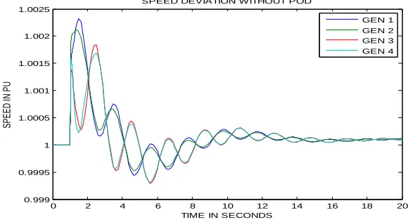
The Modal analysis is used in identifying the group of generators that constitute an area. Table 2 shows the list of left eigenvectors for the speed components of the system eigenvalues, Figure 3 shows the compass plot of the right eigenvectors of the speed state components of the 4 generators in the system. The plot is an indicator of the machines oscillating coherently in an area for the selected poor damped inter-area mode 3 in Table 1. Table 1: System Dominant Eigenvalues with and without POD
S/No EIGENVALUE WITHOUT POD
DAMPING RATIO WITHOUT POD
EIGENVALUE WITH POD
DAMPINGRATIO WITH POD 1 -0.8752 + 6.2808i 0.1380 -0.8628 + 6.2597i 0.1365
2 -0.9760 + 6.5082i 0.1483 -0.9572 + 6.4659i 0.1464
3 -0.2428 + 3.7434i 0.0647 -0.7690 + 3.1067i 0.2630
Table 2: Right Eigenvectors of Speed State Component Generators Left Eigenvectors
1 0.0621 - 0.0256i
2 0.3749 - 0.4097i
3 -0.0227 - 0.1096i 4 -0.4352 + 0.2327i
Figure 3: Mode Shape of Kundur two Area System
0.2 0.4
0.6
30
210
60
240
90
270 120
300 150
330
180 AREA 2 0
GEN 3 AND 4 AREA 1
B. Result of Dynamic Simulation
Figures 4 and 5 shows the result of dynamic simulation with three phase fault on Bus 11 for 0.05 sec. The effect of the damping on machine deviation from 1 pu without and with Power Oscillation Damper is clearly revealed.
Figure 4: Speed Deviation of the Four Machines without POD
Figure 5: Speed Deviation of the Four Machines With POD
C. Result of Modal Analysis Test System 2
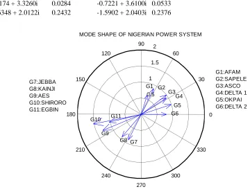
The Modal analysis is used in identifying the group of generators that constitute an area. Figure 6 shows the compass plot of the right eigenvectors of the speed state components of the 11 generators in the system. The plot is an indicator of the machines oscillating coherently in an area for the selected poor damped inter-area mode 1 in Table 3.
Table 3: System Eigenvalues and Dampng Ratios
--- EIGENVALUES DAMPING EIGENVALUES DAMPING
WITHOUT POD RATIO WITH POD RATIO
1 -1.6407 + 8.4932i 0.0219 -1.7438 + 8.5469i 0.0229 2 -0.5812 + 8.1009i 0.0088 -0.5544 + 8.0712i 0.0085 3 -1.0184 + 8.2293i 0.0148 -0.9708 + 8.0572i 0.0147 4 -1.0199 + 7.9320i 0.0159 -0.9688 + 7.7068i 0.0161 5 -0.6920 + 6.3196i 0.0171 -0.6600 + 7.1578i 0.0128 6 -0.9109 + 6.1541i 0.0235 -0.7063 + 6.2629i 0.0178
0 2 4 6 8 10 12 14 16 18 20
0.999 0.9995 1 1.0005 1.001 1.0015 1.002 1.0025
TIME IN SECONDS
S
P
E
E
D
IN
P
U
SPEED DEVIATION WITHOUT POD
GEN 1 GEN 2 GEN 3 GEN 4
0 2 4 6 8 10 12 14 16 18 20
0.9995 1 1.0005 1.001 1.0015 1.002
TIME IN SECONDS
SP
EE
D
IN
P
U
SPEED DEVIATION WITH POD
9 -0.3174 + 3.3260i 0.0284 -0.7221 + 3.6100i 0.0533 10 -1.6348 + 2.0122i 0.2432 -1.5902 + 2.0403i 0.2376
Figure 6: Mode shape of Nigerian Power System D. Result of Dynamic Simulation of Nigerian Power System
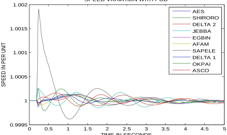
The Dynamic Simulation was performed with and without POD. Figures 7 and 8 shows the speed deviation of the 11 generators from 1 pu without and with POD.
Figure 7: Speed Deviation of the 11 Generators in the System without POD 0.5
1 1.5
2
30
210
60
240
90
270 120
300 150
330
180 0
MODE SHAPE OF NIGERIAN POWER SYSTEM
G6 G5
G4 G3 G2 G1
G7 G8 G9
G10 G11
G1:AFAM G2:SAPELE G3:ASCO G4:DELTA 1 G5:OKPAI G6:DELTA 2 G7:JEBBA
G8:KAINJI G9:AES G10:SHIRORO G11:EGBIN
0 0.5 1 1.5 2 2.5 3 3.5 4 4.5 5
0.999 0.9995 1 1.0005 1.001 1.0015 1.002 1.0025
TIME IN SECONDS
SP
EE
D
IN
P
ER
U
NI
T
SPEED VARIATION W ITHOUT POD
Figure 8: Speed Deviations of the 11 Generators in the System with POD
VII. CONCLUSION
In this work the Nigerian national grid is embedded UPFC controller that is equipped with Power Oscillation Damper, this constitutes the main case study system. The methods of Eigenvalue analysis, modal analysis and dynamic simulations, were deployed to show the impact of this damping method on Machine speed deviations. The results obtained are clear indications of the effectiveness of this proposed method.
REFERENCES
[1] G. Rogers, Power System Oscillations, Kluwer Academic Publishers, December 1999.
[2] G. H. Golub and H. A. van der Vorst, “Eigenvalue computation in the 20th century,” in J. Comput. and Appl. Math., vol. 123, no. 1–2, pp. 35–65, Nov. 2000.
[3] G. Angelidis and A. Semlyen, “Efficient calculation of critical eigenvalue clusters in the small signal stability analysis of large power systems,” IEEE Trans. Power Syst., vol. 10, no. 1, pp. 427–432, Feb. 1995.
[4] G. Angelidis and A. Semlyen, “Improved methodologies for the calculation of critical eigenvalues in small signal stability analysis,” IEEE Trans. Power Syst., vol. 11, no. 3, pp. 1209– 1217, Aug. 1996.
[5] L. T. G. Lima, L. H. Bezerra, C. Tomei, and N. Martins, “New methods for fast smallsignal stability assessment of large scale power systems,” IEEE Trans. Power Syst., vol. 10, no. 4, pp. 1979–1985, Nov. 1995.
[6] V. Ajjarapu and B. Lee, “Bifurcation theory and its application to nonlinear dynamical phenomena in an electrical power system,” IEEE Trans. Power Syst., vol. 7, no. 1, pp. 424–431, Feb. 1992.
[7] Nwohu, M. N., (2007). Voltage Stability Enhancement of the Nigerian Grid System using FACTS devices. Ph. D. Dissertation, ATBU Bauchi. Unpublished.
[8] P. Kundur, Power System Stability and Control, EPRI, McGraw-Hill, 1994, ISBN 0-07- 035958-X
[9] H.M. Ayres a, I. Kopcak b,*, M.S. Castro a, F. Milano c, V.F. da Costa a “A didactic procedure for designing power oscillation dampers of FACTS devices” Simulation Modelling Practice and Theory 18 (2010) 896–909. www.elsevier.com/locate/simpat
[10] F.L. Pagola, L. Rouco. and I.J. Perez-Arriaga, “Analysis and Control of Small-Signal Stability in Electric Power Systems by Selective Modal Analysis,” Eigenanalysis and Frequency Domain Methods for System Dynamic Performance, IEEE publication 90TH0292-3-PWR.
[11] M. E. Aboul-Ela, A. A. Salam, J. D. McCalley and A. A. Fouad, "Damping controller design for power system oscillations using global signals", IEEE Transactions on Power System, Vol 11, No. 2, May 1996, pp 767-77
0 0.5 1 1.5 2 2.5 3 3.5 4 4.5 5
0.9995 1 1.0005 1.001 1.0015 1.002
TIME IN SECONDS
S
P
E
E
D
I
N
P
E
R
U
N
IT
SPEED VARIATION WITH POD