Operational tsunami modelling with TsunAWI – recent developments and applications

(1)

Nat. Hazards Earth Syst. Sci., 13, 1629–1642, 2013 www.nat-hazards-earth-syst-sci.net/13/1629/2013/ doi:10.5194/nhess-13-1629-2013

EGU Journal Logos (RGB)

Advances in

Geosciences

Open Access

Natural Hazards

and Earth System

Sciences

Open Access

Annales

Geophysicae

Open Access

Nonlinear Processes

in Geophysics

Open Access

Atmospheric

Chemistry

and Physics

Open Access

Atmospheric

Chemistry

and Physics

Open Access Discussions

Atmospheric

Measurement

Techniques

Open Access

Atmospheric

Measurement

Techniques

Biogeosciences

Open Access Open Access

Biogeosciences

Discussions

Climate

of the Past

Climate

of the Past

Discussions

Earth System

Dynamics

Earth System

Dynamics

Discussions

Geoscientific

Instrumentation

Methods and

Data Systems

Open Access

_{Geoscientific}

Instrumentation

Methods and

Data Systems

Geoscientific

Model Development

Geoscientific

Model Development

Discussions

Hydrology and

Earth System

Sciences

Open Access

Hydrology and

Earth System

Sciences

Ocean Science

Discussions

Solid Earth

Discussions

The Cryosphere

Natural Hazards

and Earth System

Sciences

Open Access

Discussions

Operational tsunami modelling with TsunAWI – recent

developments and applications

N. Rakowsky, A. Androsov, A. Fuchs, S. Harig, A. Immerz, S. Danilov, W. Hiller, and J. Schr¨oter

Alfred Wegener Institute, Helmholtz Centre for Polar and Marine Research, Bremerhaven, Germany

Correspondence to: N. Rakowsky ([email protected])

Received: 30 November 2012 – Published in Nat. Hazards Earth Syst. Sci. Discuss.: – Revised: 21 February 2013 – Accepted: 1 March 2013 – Published: 22 June 2013

Abstract. In this article, the tsunami model TsunAWI

(Al-fred Wegener Institute) and its application for hindcasts, in-undation studies, and the operation of the tsunami scenario repository for the Indonesian tsunami early warning system are presented. TsunAWI was developed in the framework of the German-Indonesian Tsunami Early Warning System (GITEWS) and simulates all stages of a tsunami from the ori-gin and the propagation in the ocean to the arrival at the coast and the inundation on land. It solves the non-linear shallow water equations on an unstructured finite element grid that allows to change the resolution seamlessly between a coarse grid in the deep ocean and a fine representation of coastal structures. During the GITEWS project and the following maintenance phase, TsunAWI and a framework of pre- and postprocessing routines was developed step by step to pro-vide fast computation of enhanced model physics and to de-liver high quality results.

1 Introduction

The devastating tsunami in December 2004 triggered numer-ous activities aiming at the installation of a tsunami early warning system in the Indian Ocean. Since the time avail-able for early warning is very short, especially along the In-donesian coast facing the Sunda Trench, first estimates of the tsunami impact after an earthquake are based on precom-puted tsunami simulations. These can rely only on a model thoroughly tuned and verified following the guidelines based on Synolakis et al. (2007, 2008). Furthermore, for warning systems in the Indian Ocean, the implementation plan (IOC, 2008) demands to benchmark the operational models accord-ing to these guidelines.

In the framework of the German-Indonesian Tsunami Early Warning System (GITEWS), the tsunami modelling group at AWI (Alfred Wegener Institute) has developed the operational model code TsunAWI and provided the warning centre at the Indonesian Agency for Meteorology, Climatol-ogy, and Geophysics (BMKG), Jakarta, Indonesia, with a repository of 3470 prototypic tsunami scenarios. Since the start of GITEWS in 2005, the warning system was con-structed and improved step by step, integrating the daily ex-periences at the warning centre, and so was the TsunAWI code developed. In this article, we want to highlight some aspects of this process of TsunAWI developing from a re-search model to an operational code with a framework of pre-and postprocessing routines. The development of TsunAWI started as a spin-off of the ocean model FESOM (Finite El-ement Sea-Ice Ocean Model) (Wang et al., 2012b, and refer-ences therein), from which it inherited the main structure, the finite element discretisation, and some core routines. The first step was to drastically reduce the model physics, e.g. to elim-inate the vertical dimension, the temperature and the salinity. On the other hand, inundation, that can be neglected in large scale ocean modelling, had to be implemented.

The code TsunAWI simulates all stages of a tsunami from the source to propagation and run-up by solving the non-linear shallow water equations discretised with finite ele-ments on a two-dimensional unstructured triangular grid. This discretisation is very flexible with respect to resolution and allows for an excellent representation of complicated coastlines and bathymetry. Other tsunami models also take the advantages of unstructured grids, though usually pared with finite volume discretisations (e.g. ANUGA, Roberts et al., 2007). As the price for the unstructured mesh is a less efficient implementation, other models rely on regular

(2)

grids, which may be nested to resolve areas of interest, the finite difference model TUNAMI-N3 (Tohoku University’s Numerical Analysis Model for Investigation of Near-field Tsunami Number 3) (Imamura et al., 2006) being a well known example.

In Sect. 2, the basics of TsunAWI are introduced, namely the underlying shallow water equations, the discretisation with finite elements, and some implementation issues. Sec-tion 3 presents results on the 2004 Indian Ocean tsunami. The tsunami scenario repository built for GITEWS is described in Sect. 4. Section 5 concludes with a look at ongoing and planned research.

2 The tsunami simulation code TsunAWI

2.1 The governing equations

The non-linear shallow water equations (SWE)

The tsunami simulation code TsunAWI is based on the rotat-ing non-linear SWE given by the vertically averaged equa-tions of motion and continuity. We consider the boundary value problem in Cartesian coordinates (x, y)∈ in the plane domainwith boundary∂at the timet∈ [0, T]

∂v

∂t +fk×v+(v·∇)v+g∇ζ

+r

Hv|v| − ∇(Kh∇v)=0, (1) ∂ζ

∂t + ∇ ·(Hv)=0 (2)

for the horizontal velocity vector v=(u, v) and the total water depthH=h+ζ >0 as the sum of the unperturbed water depth h and the surface elevation ζ. Furthermore, ∇ =∂

∂x, ∂ ∂y

denotes the gradient operator,f the Coriolis parameter,k the vertical unit vector,r the bottom friction coefficient, andKhthe eddy viscosity coefficient.

Boundary conditions

On the solid part of the boundary∂1, the condition vn

∂1 =0 (3)

for the velocityvn=v×nnormal to∂1 is imposed. For

the open part ∂2, Oliger and Sundstr¨om (1978) derived 0 (v, ζ )|_∂

2 =21with the operator of the boundary condi-tion0and a vector function21determined by the boundary

regime, differing for inflow and outflow. In practice, the full information on the open boundary is unavailable, and one option is to impose the boundary condition on the elevation

ζ|_∂

2 =9(x, y, t ). The accuracy of this approach was analy-sed by Androsov et al. (1995). For most tsunami simulations, the radiation boundary condition

vn

∂2 =

r g

H ζ (4)

is implemented in TsunAWI providing free linear wave pas-sage through the open boundary, given the Coriolis acceler-ation plays only a small role (for a review of several open boundary conditions see Røed and Cooper, 1986). Further-more, as TsunAWI operates on unstructured grids, the open boundary can be replaced by a coarse global grid with a finely resolved focus on the region of interest.

Initial conditions

Initial conditions can be taken from various sources, e.g. Okada parameters (Okada, 1985) from geological sur-veys for hindcasts, or prototypic ruptures for the Sunda Arc provided by the German Research Centre for Geosciences (GFZ) for GITEWS (RuptGen, Babeyko et al., 2008, 2010). Especially for hindcasts, TsunAWI allows to elevate the ocean bottom and surface repeatedly within several time steps, following the time frame of the source model. Usu-ally, only an initial sea surface heightζ0is given, while the

velocity is assumed to be zero, but it is also possible to supply an initial velocity field additionally, e.g. derived from a land slide model as provided by Androsov and Voltzinger (2005).

Bottom friction

Manning bottom friction with a constant parameter is chosen for most calculations. Alternatively, a value varying with the surface structure can be provided.

2.2 Numerical method

Finite element method

Finite element methods are widely used in studies of wave generation and propagation in different fields of fluid dy-namics. They are often employed to simulate propagation of long waves such as ocean tides and tsunamis in the ocean in the framework of shallow-water equations, e.g. Kienle et al. (1987); Greenberg et al. (1987); Baptista et al. (1993). The main reason to choose finite elements is the computational mesh that can be adapted to cover basins with irregular bot-tom topography and coastlines. The spatial discretisation of TsunAWI is based on the finite element approach by Hanert et al. (2005) with modifications like added viscous and bot-tom friction terms, corrected momentum advection terms, ra-diation boundary condition, and nodal lumping of mass ma-trix in the continuity equation. The basic principles of dis-cretisation follow Hanert et al. (2005) with linear conform-ing elementsP1for sea surface heightζ and water depthh,

(3)

Leap-frog time stepping scheme

Simulation of tsunami wave propagation benefits from an explicit time discretisation. Indeed, numerical accuracy re-quires relatively small time steps, which reduces the main advantage of implicit schemes. Furthermore, modelling the inundation processes requires very high spatial resolution in coastal regions and consequently a large number of nodes, drastically increasing computational demands for an implicit time discretisation.

The leap-frog discretisation was chosen as a simple and easily implemented method. We rewrite Eqs. (1) and (2) in time discrete form

vn+1₋_vn−1

24t +fk×v

n₊ _vn_·∇

vn+g∇ζn

+ r

Hn|v

n_|_vn+1_{− ∇}_K h∇vn−1

=0,

(5)

ζn+1−ζn−1

24t

+ ∇ · Hnvn

=0 (6)

with the time step length4t and the time indexn. The leap-frog three-time-level scheme provides second-order accuracy and is neutral within the stability range. This scheme, how-ever, has a numerical mode, which is removed by the stan-dard Robert–Asselin filter. Notice that friction and viscosity contributions deviate from the usual leap-frog method.

Momentum advection scheme

Because of the discontinuous character of velocity represen-tation, special care is required with respect to the implemen-tation of the momentum advection. Earlier experiments with

P₁NC−P1code revealed problems with spatial noise and

in-stability of the momentum advection when the discretisation is used as described by Hanert et al. (2005). A modified im-plementation without upwinding terms was found to work well when paired with rather high viscous dissipation to re-move small-scale noise in the velocity field. In addition, the implementation of the momentum advection forP₁NC velo-cities involves cycling over edges in the numerical code, in addition to cycling over elements to assemble the elemen-tal contributions. This leads us to a simpler approach, which provides a smoothing of the velocity field while removing edge contributions.

According to this approach, prior to calculating the advec-tion term in the momentum equaadvec-tion, we project the veloc-ity fromP₁NC toP1space in order to smooth it. This pro-jection becomes numerically efficient by nodal quadrature (lumped mass matrix). The projected velocity is then used to estimate the advection term. Finally, the result is multi-plied with aP₁NCbasis function and integrated over the do-main (Maßmann et al., 2008). This results in a very stable be-haviour.

Viscosity

The coefficientKhfor the horizontal viscosity is determined

by a Smagorinsky parameterization

Kh=csmag4x4y4t

r

(ux)2+ vy 2

+1

2 uy+vx

2

(7)

(Smagorinsky, 1963). Optionally, the standard linear visco-sityKh=clin4x4ymay be chosen for comparison or to save computation time. The advantages of Smagorinsky viscosity are demonstrated in the simulation of the Okushiri channel experiment test case (Androsov et al., 2008).

Wetting and drying

For modelling wetting and drying, we use a moving bound-ary technique based on the “dry node concept” developed by Lynett et al. (2002). The idea is to exclude dry nodes from the solution, but to extrapolate the elevation to the dry nodes from their wet neighbours. As this scheme is neutrally stable, it requires horizontal viscosity in places of large gradients of the solution. The Smagorinsky viscosity (7) fulfills this task while keeping the dissipation on a level that does not affect the quality of the solution.

The implementation in TsunAWI showed that in order to retain stability it has to be decided which values to extrapo-late and how. Finally, linear extrapolation was chosen for the gradient∇ζ and the sea surface heightζ at dry elements and nodes. Furthermore, all other values at dry nodes, elements, and edges are excluded from further computations.

In the first versions of TsunAWI, the extrapolation scheme was not always stable at complicated coastlines when the mesh did not resolve the geography smoothly enough. This could lead to local numerical artefacts like spurious spikes in the amplitude or initial waves of high frequency in the far field of the source. Due to the fractal nature of many coastlines, this problem cannot be solved by mesh generation alone and was handed over to the postprocessing routines. With growing experience, the problem could be solved for TsunAWI, which now runs stably if the time step and mesh resolution are chosen appropriately.

Mesh generation

(4)

all triangles fulfill the criterion 4x≤min

cCFL

p gh, cg

h

∇h

. (8)

As the Triangle output is not smooth enough for numerical experiments, several smoothing iterations are applied. Each iteration consists of edge swapping, torsion smoothing, and linear smoothing. Torsion smoothing tries to adjust the an-gles around each node, linear smoothing acts on the distance between nodes. These strategies are described in Frey and Field (1991).

Code optimisation and parallelisation

The operational version of TsunAWI is parallelised with OpenMP (Open Multiprocessing) by defining parallel re-gions in the numerically most demanding parts of the code and splitting up the corresponding loops, thus sharing the load to the cores involved. The implementation in this ap-proach needs smaller changes than a fully parallel MPI (Mes-sage Passing Interface)-implementation, and proves to be nu-merically efficient, if data locality is ensured.

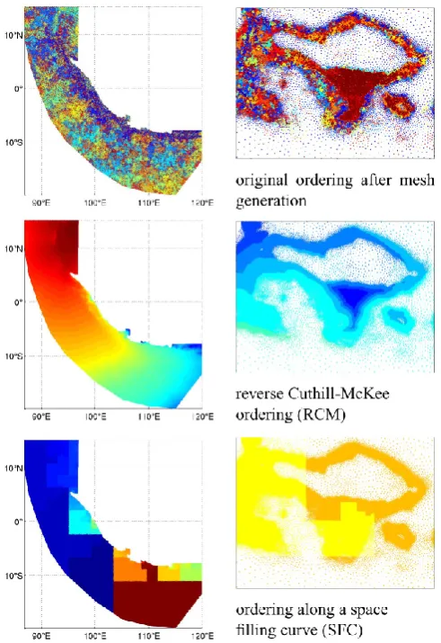
In fact, already in a serial code, data locality is crucial for the performance. In particular the representation of vari-ables in an unstructured mesh, if not constructed carefully, can result in many cache misses during calculation and con-siderably slow down the code. For TsunAWI simulations we therefore order the variables along a space filling curve (SFC, for triangular meshes with regular structure see Bader et al., 2008), which guarantees good data locality on all levels of the memory hierarchy by construction. The ordering is visu-alised in Fig. 1, the effect on the computation time is shown in Table 1. Results for one commonly used ordering tech-nique, reverse Cuthill-McKee (RCM, George and Liu, 1981), are given for comparison.

Pre- and postprocessing

Preprocessing for TsunAWI runs is dominated by producing a smooth computational grid that resolves the domain in the desired accuracy. In the first model runs, the time step length is tuned to be as long as possible while keeping the scheme stable. For a small number of runs in one setting, e.g. for a hindcast, the preliminary steps pass over into the main simulation. However, for repository calculations with several thousand scenarios, scripts have to be provided to automate the runs on large Linux clusters. While in the early days of GITEWS, TsunAWI computation was expensive compared to data storage, the ratio is now vice versa. We therefore now reduce the amount of data beforehand, e.g. by decid-ing at which locations a timeline is really needed in addition to global values like maximum amplitude, arrival time, and maximum flux.

TsunAWI output is written in netCDF (Common Data For-mat), which is standard in oceanography, but cannot be dis-played by GIS applications. A set of postprocessing scripts

Fig. 1. Three different orderings of variables in the regional Indone-sian grid, from dark blue for the first node to dark red for the last one (2.3 million). On the left for the whole domain, on the right a zoom at Bali region reduced to 16 colours emulating the distribution on 16 OpenMP threads.

Table 1. Computational time (s) for one TsunAWI time step, re-gional Indonesian scenario, on one blade of the SGI Altix UV at HLRN, 2×Intel Xeon 5570 (8 Cores, 2×hyperthreading).

OpenMP threads

1 2 4 8 16 32

orig. 3.84 2.16 1.48 0.89 0.52 0.40 RCM 1.64 1.12 0.59 0.35 0.20 0.19 SFC 1.47 0.90 0.51 0.31 0.17 0.14

and routines extracts the data products and converts them to shapefile format needed by the warning system.

(5)

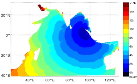
Fig. 2. Arrival time with a threshold of 2 cm for a minor tsunami scenario, Mw=8.0. In the regions marked in black, the fixed

threshold is never reached, at some, it is reached by the second or third wave crest.

we therefore chose a relative threshold of 10 % of the lo-cal maximum amplitude, see Fig. 3. Still, islands and other complicated geographical settings can produce discontinu-ous arrival times and there is no other way but checking the isochrones of each scenario manually.

3 Application: hindcast of the Indian Ocean tsunami in

December 2004

TsunAWI is still under development and the performance and model results must be constantly evaluated to ensure a consistent and stable code. Validation needs to be performed on several levels, like consistency and convergence, bench-marks in idealised settings with well defined results as pro-posed by Synolakis et al. (2007, 2008), and comparisons with real cases with measured data. This section focusses on one hindcast in detail, comparing model results with data from various sources. Of course, other major tsunami events like Chile 2010 and Japan 2011 and all Indonesian tsunamis since 2005, like Bengkulu 2009 and Mentawai 2010, have also been used for TsunAWI validation and parameter calibra-tion. The validation with the benchmarks by Synolakis et al. (2007, 2008) is performed whenever the TsunAWI code has been extended or enhanced with new model physics or nu-merical techniques, see e.g. Androsov et al. (2008) for re-sults on the sloping beach and Okushiri channel test cases, and Wekerle et al. (2010) for the effect of model parameters, e.g. mesh resolution, and model physics, e.g. non-linear ad-vection, on the Okushiri field test case. A paper summarizing the validation for the current state of TsunAWI in GITEWS is in preparation.

For the tsunami generated by the great Sumatra–Andaman earthquake on 26 December 2004, a large amount of data are available. In this section, model comparisons with observa-tions from satellite altimetry, tide gauge records, and field surveys are discussed. The results are closely related to the studies in Harig et al. (2008), where additional information can be found.

Fig. 3. Arrival time for the same scenario as in Fig. 2 but with a relative threshold of 10 % of the local maximum amplitude.

Topography and bathymetry data

Topography and bathymetry data are based on several sources. The General Bathymetric Chart of the Oceans (GEBCO) data are globally available with 30 arc seconds res-olution and are used as initial topographic and bathymet-ric information. It is replaced by more precise data wher-ever available. Bathymetric data are locally improved by ship measurements and nautical charts. Topographic infor-mation is improved by the Shuttle Radar Topography Mis-sion (SRTM) data, which are freely available at a resolu-tion of 90 m, however the vertical accuracy is usually not sufficient for model studies with inundation. For Indonesia, the SRTM data were additionally processed by the German Aerospace Agency (DLR) and provided at a resolution of 30m. In the Aceh region, additional bathymetric and topo-graphic data were provided by BPPT Jogyakarta.

Source model

(6)

Subfault Strike Dip angle Initial Slip [m] rupt. time

A 340◦ 10◦ 0 min 21.1±5.0 B 340◦ 10◦ 1 min 0.0±0.0 C 340◦ 10◦ 1 min 22.9±6.7 D 340◦ 10◦ 3 min 4.2±3.1 E 340◦ 10◦ 3 min 9.6±1.3 F 340◦ 10◦ 5 min 5.1±2.7 G 340◦ 10◦ 5 min 0.0±0.0 H 340◦ 10◦ 7 min 11.2±0.9 I 340◦ 10◦ 7 min 13.9±2.6 J 340◦ 10◦ 8 min 14.5±2.1 K 340◦ 3◦ 10 min 7.3±0.4 L 10◦ 17◦ 12 min 1.1±0.3

Fig. 4. Subfaults as proposed by Tanioka et al. (2006). The rup-ture area is decomposed into 12 subregions. With a ruprup-ture speed of 1.7 km s−1, the whole rupture process takes 12 min. Faults B and G have zero slip in our experiments and are not displayed. For the red faults, a different strike angle is examined.

of the 2004 tsunami optimised with respect to selected data. In the present study we are not aiming at source optimisation, rather we would like to highlight the sensitivity of model re-sults with respect to small changes of source parameters.

Model set-up

The simulation code TsunAWI was employed on a compu-tational mesh with 5 million nodes and 10 million triangles. The whole Indian Ocean is covered with a resolution range between 15 km in the deep ocean and 40 m in the Aceh re-gion in northern Sumatra, see Fig. 5. The finest resolution enforces a time step of 0.5 s, and the model is integrated for 10 h. This rather short integration time was just enough to compare with most measurements, and the focus was to per-form a larger number of runs for different combinations of finite fault solutions and model parameters. In the positions

Fig. 5. Tide gauge locations and mesh density in the model domain. The green areas are land nodes which are initially dry. The resolu-tion ranges from 15 km in the deep ocean to 40 m in Aceh, Sumatra.

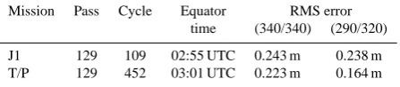
Table 2. Satellite missions Jason 1 (J1) and Topex/Poseidon (T/P). The last columns quantify the RMS error obtained in the TsunAWI scenarios with different strike angles in subfaults A and C (Fig. 4) during the approx. 10 min of the satellite overpasses.

Mission Pass Cycle Equator RMS error time (340/340) (290/320)

J1 129 109 02:55 UTC 0.243 m 0.238 m T/P 129 452 03:01 UTC 0.223 m 0.164 m

along the satellite tracks, the model state is written to a file every second to allow for a comparison between model and satellite altimetry data. Additional information on model set-up and initialization can be found in (Harig et al., 2008).

Satellite altimetry

(7)

Fig. 6. Model snapshot after 2 h. Sea surface elevation together with the satellite tracks Jason 1 and Topex/Poseidon.

Fig. 7. Tsunami signal extracted from the satellite tracks Jason 1 and Topex/Poseidon, and model results along the tracks interpolated in space and time.

matching and lowers the root-mean-square (RMS) errors as indicated in Table 2.

However, it has to be noted that Allen and Greenslade (2012) have recently pointed out that the RMS error is not necessarily the best parameter to compare model results, be-cause it may be to sensitive to outliers.

Inundation

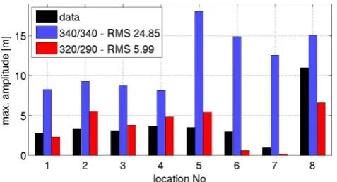
After the event in December 2004, several field surveys ex-amined the run-up and maximum flow depth in the affected regions. In the area of Banda Aceh, which was most heavily hit, eight locations with well documented field measurements were chosen to be compared with model run-up. As flow

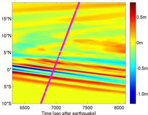
Fig. 8. Hovm¨oller diagram for the modelled sea surface elevation of the Jason 1 track (Fig. 6). The model results corresponding to the satellite observations (Fig. 7) are interpolated in space and time.

Fig. 9. Positions of field measurements and flowdepth obtained with Manning numbern=0.03 and original Tanioka source. The red line indicates the inundated area as it was determined from satellite im-ages by DLR.

depth and run-up depend heavily on the prescribed rough-ness parameterization, several experiments with identical ini-tial conditions and different values for the Manning parame-ter were conducted. In all cases, a constant manning number was applied in the whole domain.

(8)

Fig. 10. Flow depth comparison in locations marked in Fig. 9 for different roughness parametersnand the modified source (strike angle 290/320).

Fig. 11. Flow depth comparison in locations marked in Fig. 9 for strike angles of plates A/C set to 340/340 and 290/320.

of the different strike angles in the southern subfaults on the inundation simulation RMS error is shown in Fig. 11. Also in this respect, the modified orientation improves the results considerably. In fact, the unsatisfactory inundation result ob-tained with the original source was the reason to test the strike angles proposed by Hirata et al. (2006) for the southern subfaults, because they have the largest impact on the inun-dation in Banda Aceh.

Tide gauge records

The Indian Ocean tsunami was registered by tide gauges worldwide. Since arrival time and estimated amplitude are among the most important warning products, good matching between model results and tide gauge measurements of ar-rival times and the height of the leading wave crest is impor-tant. Figure 12 summarises the time series in some locations throughout the Indian Ocean. The comparisons between tide gauge records and model results generally match well with respect to arrival time. The height of the leading crest is sometimes underestimated, however, in most of the locations the agreement is very good. The orientation of the south-ern subfaults does not influence the results at far distances such as Salalah and Lamu, and the matching in Colombo is slightly better with the uniform values (340/340). This is consistent with the derivation of these strike values, as this station was used for optimisation in Tanioka et al. (2006).

(9)

Summary of the Indian Ocean study

Summing up, TsunAWI is able to reproduce observational re-sults on several scales of wave propagation. In our approach with unstructured meshes, both the large scale propagation throughout the Indian Ocean and the inundation in a selected area with high resolution can be combined within a single model run. However, the results strongly depend on the qual-ity of the source model.

4 Application in the German-Indonesian Tsunami

Early Warning System (GITEWS)

The German-Indonesian Tsunami Early Warning System was founded after the devastating Indian Ocean tsunami, in 2004, as a joint project of German research institutes as well as Indonesian institutes and authorities. In 2005, Indonesia and Germany agreed in a joint declaration to develop a warn-ing system coordinated by the UNESCO Intergovernmental Oceanographic Commission. The system was inaugurated in 2008, evaluated in 2010 by an international commission, and handed over to the Indonesian government in 2011. In the ongoing project for training, education and consulting for the tsunami early warning system (PROTECTS), the Indonesian staff are trained in the use and maintenance of all compo-nents.

4.1 Tsunami scenario repository for GITEWS

The Indonesian warning system meets the challenge of near field warning with extremely short warning time. As tsunamigenic earthquakes originate close to the shore, the time between a seismic event and the issue of a warning is limited to just a few minutes. The early warning system therefore relies on a repository of tsunami scenarios precom-puted with the tsunami model TsunAWI. To speed up the processing in a warning situation, an index database is ex-tracted offline. It contains data products for all scenarios like virtual sensor data and shapefiles with estimated maximum amplitude and arrival times at coastal forecast zones, and isochrones.

Warning system architecture

Data of various sensors, such as the seismic stations ana-lysed by SeisComP (Seismological Communication Proces-sor), global positioning system (GPS) sensors as well as data from tide gauges and buoys, are collected via the Tsunami Service Bus (TSB, Fleischer et al., 2010), and distributed to the Decision Support System (DSS, Steinmetz et al., 2010), which triggers the Simulation System (SIM) with the avail-able sensor data. On this basis, the SIM delivers a set of best matching scenarios. The DSS performs a worst case aggrega-tion over these scenarios and visualizes expected maximum amplitudes and arrival times for the Indonesian coasts. The

system is installed at the warning centre in Jakarta, Indone-sia, and assists the chief officers on duty to assess the poten-tial tsunami risk and to disseminate warnings to governmen-tal institutions, local disaster management, action forces, and media.

Tsunami scenario repository

In the beginning of the GITEWS project, emphasis was put on getting the warning system operational as fast as possi-ble and enhancing the running system step by step. For the tsunami scenario repository (TSR), this approach was fol-lowed and as soon as good bathymetry data and a rupture model (RuptGen by Babeyko et al., 2010) had become avail-able, first scenarios were computed with a first version of TsunAWI based on the linear SWE and with linear visco-sity. As computation and quality control took about half a day per scenario, the repository first covered only a smaller number of epicentres and magnitudesMw=8.0,8.5,9.0. In

the daily routine at the warning center, it soon turned out that scenarios for lower magnitudes Mw∈[7.2,8.0] were most

urgently needed, because smaller earthquakes occur far more frequently and their tsunami potential is much harder to as-sess. Therefore, the TSR was extended to contain lower mag-nitudesMw.

In early 2011, all scenarios in the TSR were replaced in one step by new ones that were calculated with the enhanced TsunAWI code including non-linear advection, Smagorinsky viscosity, improved inundation scheme, and with initial con-ditions derived from an extended version of RuptGen (Rup-ture Generator) offering also rup(Rup-tures closer to the coast. The TSR now contains 3470 scenarios for prototypic rup-tures with magnitudes evenly spaced in the range ofMw= 7.2,7.4, . . . ,9.0 on 528 different epicentres, see Fig. 13.

These scenarios are used in the warning situation as well as for risk analysis and hazard maps, as long as no simulations with higher resolution are available. For earthquakes with epicentres outside the area covered by the TSR, e.g. in the Banda Sea, a tsunami simulation is performed within 1 min computation time by the model EasyWave (Babeyko, 2012). EasyWave discretises the linear SWE in deep water on a reg-ular coarse grid and estimates the amplitude at the coast by Green’s law. Currently, we are preparing TsunAWI scenarios for epicentres in the eastern Sunda Arc.

(10)

Fig. 13. Tsunami scenario repository for GITEWS. Scenarios for up to ten different magnitudesMw=7.2,7.4, . . . ,9.0 are calculated at

each of the 528 positions marked with red dots, resulting in 3470 scenarios in total.

The dense net of scenarios allows to evaluate the effect of small changes in epicentre and magnitude as shown in Fig. 14 for artificial mareograms for the harbour of Padang, Sumatra. The logarithmic energy scale of the magnitude is clearly illustrated by the upper mareogram. The lower graph shows more complex features due to varying epicentres on a line perpendicular to the trench. With the magnitude fixed to

Mw=8.0, the tsunamis originating closest to the coast have the lowest impact. On the one hand, this is due to the initial conditions generated by RuptGen, which assumes a source depth of 0 km at the trench increasing up to 100 km under the main islands. A second factor determining the strength of the tsunami is the height of the water column at the origin, which is small in coastal regions.

Epicentres to the southwest off the coast yield increas-ing wave heights in Padang, until the Mentawai islands are reached. Farther west, the corresponding tsunami is no longer trapped in reflections between Sumatra and the islands, re-lieving the situation for Padang.

SIM selection algorithm

The selection algorithm implemented in the Simulation Mod-ule (SIM) combines the available sensor data to acquire a set of best matching scenarios to an earthquake event. By basing the selection on different sensor types, uncertainties result-ing from inaccurate measurements and errors in the tsunami model are reduced. A more detailed overview of the SIM is given in Behrens et al. (2010).

Originally, the so-called matching values generated for each sensor type for a scenario were accumulated in an over-all weighted sum. However, the experiences with real sensor data in the GITEWS project showed that each sensor group has to be regarded separately with its characteristics in mind. The weighted sum has therefore been replaced by a stepped

approach starting with seismic data delivering the most ro-bust values, followed by GPS data.

The algorithm takes the tectonic structure of the Sunda Arc into account. For the preselection of scenarios based on seis-mic data, an elliptic area around the measured epicentre is constructed, see Fig. 15. The dimension of the ellipse de-pends on the measured magnitudeMw with the long ellipse

axis given by

rL=max100.5[Mw+0.3]−1.8_km_,_{180 km}_. ₍₉₎ The lower value of 180 km ensures that at least one scenario is covered by the ellipse. The long axis is constructed parallel to the trench.

The second important sensor class in GITEWS are GPS dislocation vectors. The GPS measurements are fast and re-liable, thus allowing for a better estimate of the tsunami haz-ard in the first few minutes after the earthquake. For each sensor and each scenario that remains after preselection by the seismic data, the lengths of the dislocation vector from the measurement and from the corresponding scenario are compared. Scenarios for which a defined minimum number of similar GPS values has been reached are taken into ac-count for the final set of best fitting scenarios. This allows to narrow down the preselected area and to correct overesti-mated magnitudes. With more GPS sensors available, it will become possible to correct underestimated magnitudes and enlarge the seismic preselection.

Once several scenarios have been chosen for one epicen-tre, only the one with the largest magnitude within the uncer-tainty range[Mw−0.5, Mw+0.3]is kept in the list, because

the scenarios with lower magnitudes will have no relevance for the worst case aggregation in DSS processing. Hence, dis-regarding them reduces the amount of data to be processed without changing the result.

4.2 Scenarios for Indonesia as Regional Tsunami

Service Provider (RTSP)

In 2011, the warning centre at BMKG, Jakarta, became a re-gional tsunami service provider (RTSP) for the Indian Ocean together with the warning centres in India and Australia. Therefore, a second set of scenarios was required, one which covers the whole Indian Ocean with a model time of 24 h and provides a predefined set of data products like arrival times and maximum amplitudes in the forecast zones along the coast of the Indian Ocean.

(11)

0 30 60 90 120 150 180 −2

0 2 4 6

amplitude [m]

Mareograms at Padang Harbour for TSR Scenarios, Epicenter 1.8°S 99.5°E Mw=9.0,8.8,8.6,8.4,8.2,8.0,7.8,7.6,7.4,7.2

0 30 60 90 120 150 180

−2 −1 0 1 2

amplitude [m]

time after rupture [min]

Mareograms at Padang Harbour for TSR Scenarios, Mw=8.0, varying Epicenters Epicenter, see map:

Fig. 14. Influence of the magnitudeMw and of the source location on the strength of a tsunami: mareograms at Padang Harbor for

TSR-scenarios originating at the same epicentre with different magnitude (above) and with equal magnitude, but different origin (below).

102°E 104°E 106°E 108°E 110°E

9°S 7°S 5°S 3°S

1°S _{Scenario Coverage}

Trench Scenarios Epicenter

Mw≤7.7 Mw = 8.1 Mw = 8.5 Mw = 8.9 Mw = 9

Fig. 15. Seismic uncertainty ellipses for different magnitudes.

only timelines at nodes with a water depth of at least 50 m were kept to provide smooth isochrones, and after post pro-cessing, the timelines were completely deleted. Global fields of maximum amplitude and arrival times are permanently stored, together with the all preliminaries to recalculate the scenarios, if necessary.

4.3 Inundation studies for risk assessment

The focus of this section is to highlight the importance of the bottom roughness parameter. Simulations of tsunamis with identical initial conditions were carried out in a mesh with a resolution down to 5 m. The study area is Mataram, Lombok, Indonesia, and as a tsunami source, the Okada parameters for an assumed earthquake withMw=8.5, epicentre at 8.15◦S,

116.15◦E, in the back-arc region north of Lombok was pro-vided to us by the Australia-Indonesia Facility for Disaster Reduction (AIFDR).

The topography data are based on the Intermap data set with 5 m horizontal resolution, provided to us by the DLR. Two versions, a digital surface map (DSM) and a digital ter-rain map (DTM), were used. The DSM is based on a first-reflection data set and contains elevations of vegetation and buildings. In the DTM, all these features have been removed. The scenarios generated for the tsunami database are based on a coarser mesh with a resolution down to 50 m in priority regions. This resolution is a compromise between the sig-nificance of the simulation and the computational efforts. In particular, evacuation maps are based on data sets with much higher resolution, containing streets and other infrastructure. The corresponding model set-up should contain a compara-ble mesh, and in GITEWS, high resolution simulations were performed for large cities like Bengkulu, Cilacap, or Den-pasar with MIKE 21 FM (Flexible Mesh) by the German Re-search Center Geesthacht (GKSS) (Gayer et al., 2010). In these simulations, the Manning roughness parameter varies spatially according to detailed roughness maps. Details on this approach and the model can be found in Gayer et al. (2010) and citations therein.

The simulated inundation in the TSR is used for the other coastal regions. Initially, the wetting and drying scheme was only included in TsunAWI to prevent artificial wave reflec-tions at ocean basin walls. However, it soon turned out that the implemented scheme was also well suited for realistic in-undation simulation.

(12)

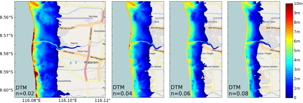
Fig. 16. Flowdepth in the model study for Mataram/Lombok (background © OpenStreetMap contributors) based on Intermap DTM with three different Manning parametersn=0.02, 0.04, 0.06, 0.08 from the left to the right panel.

Fig. 17.Flowdepth in the model study for Mataram/Lombok (back-ground © OpenStreetMap contributors) based on Intermap DSM with constant Manning valuen=0.02.

formed with the MPI-parallel research branch of TsunAWI, while the operational branch is kept as lean as possible. For the latter, with the code optimisation so far achieved and the advances in hardware near real time computing comes into reach – without reducing model physics.

680

First real time models, e.g., EasyWave (Babeyko, 2012) and RIFT (Wang et al., 2012a), allow to react in an early warning situation on the seismic information in addition to the epicenter and magnitude. Fast momentum tensor deriva-tion and GPS measurements can narrow down the potential

685

tsunami source in just a few minutes after the earthquake. To save computing time, EasyWave and RIFT employ re-duced model physics based on linear SWE in deep water with the extrapolation of the maximum amplitude to the shore by Green’s law. For the tsunami inundation hazard in the far

690

field, Tang et al. (2009) used the example of Hawaii to

con-duct a sensitivity study with respect to source parameters, bathymetry data, and grid resolution.

The computational efficiency of TsunAWI is very high re-garding model physics and resolution, but the code still has

695

to be adapted to the early warning situation. One strategy will be to coarsen grid resolution by evaluating the local CFL numbers reached in model runs in the given geographical set-ting. Another option is to employ general purpose graphics processing units (GPGPU) that make the massive

computa-700

tional power of a modern graphics accelerator available for general computing. But this option requires the maintainance of two code branches, because optimisation strategies for cache efficiency on typical CPUs and for the limited regis-ters on GPGPUs differ extremly.

705

6 Conclusions

During seven years of development, TsunAWI matured from a reseach model to an operational code with a framework of pre- and postprocessing routines. In particular, the imple-mentation of the non-linear advection and the wetting and

710

drying required the careful comparison of different schemes to achieve an algorithm that is stable without being too dif-fusive. The model has since proven its robustness, correct-ness, and efficiency in several hindcasts of tsunami events world wide and in more than 5000 scenario calculations for

715

the Indonesian Seas and the Indian Ocean. However, the ex-perience of the user in model setup and evaluation remains an important requirement for good results in tsunami modelling.

Acknowledgements. We gratefully acknowledge the contributions to the TsunAWI framework by J¨orn Behrens, Dmitry Sein, Dmitry

720

Sidorenko, Widodo Pranowo, and Chaeroni. We thank the col-leagues at DLR, Matthias M¨uck and Ralph Kiefl, for providing us with Intermap topography for Materam and with inundation ar-eas estimated from satellite images, respectively. Widjo Kongko

Fig. 16. Flowdepth in the model study for Mataram/Lombok (background © OpenStreetMap contributors) based on Intermap DTM with four different Manning parametersn=0.02,0.04,0.06,0.08 from the left to the right panel.

Fig. 17. Flowdepth in the model study for Mataram/Lombok (back-ground © OpenStreetMap contributors) based on Intermap DSM with constant Manning valuen=0.02.

heterogeneous fluid flow, which may be only poorly ap-proximated by a bottom friction parameterization. The re-sult based on DSM contains small scale features, however, since the destruction of buildings and vegetation is not taken into account, the extent of the inundation may be underesti-mated. Gayer et al. (2010) suggests the use of DTM data with detailed roughness maps. According to Gayer et al. (2010), the right panel corresponds to the situation of an urban area with partly collapsing buildings whereas the left panel corre-sponds to the situation of the whole area covered by coarse sand.

Given the vast differences displayed in Fig. 16, the results are meant to raise the awareness to the fact that the simu-lated inundation strongly depends on the friction parameters. The quality of topography data plays an even bigger role and the best suited data set and model parameterization must be chosen before hazard maps are produced. Furthermore, the

derivation of the shallow water equations (SWE) (1) and (2) is based on the assumption of a small ratio of water height to wave lengthh/λ1. If the wave is determined by very fine scale topographic features, the validity of the SWE becomes questionable. As long as the focus of such model studies lies on the inundated area alone, the limitations of the SWE might still be acceptable. In addition to the work presented here, it would be desirable to assess the limitations of TsunAWI compared to models with e.g. three dimensional simulation, non-hydrostatic flows, wave breaking, or sediment transport.

5 Outlook

TsunAWI is under constant development and our current re-search focusses on two modular additions, one for the non-hydrostatic pressure correction, the second for tidal forcing. Both aim to improve the tsunami hazard assessment.

The non-hydrostatic correction follows the approach of Walters (2005) and can be activated on demand, when coast-line geometry or steep bathymetric gradients necessitate it for realistic simulation results.

Tides are usually neglected in tsunami modelling, because a typical tsunami wave has a much shorter wave length. How-ever, simulation with TsunAWI (Androsov, 2010; Androsov et al., 2011) showed that the inclusion of tides can have a sig-nificant effect on the amplitude and phase of tsunami waves in regions with strong tidal currents or shallow bathymetry. For these experiments, a small simulation area was chosen and the tidal forcing was imposed on the boundary condi-tions. To simplify the set-up for simulations in arbitrary re-gions, TsunAWI is now extended to a global tidal model, and the region of interest is refined in the unstructured grid.

(13)

the latter, with the code optimisation so far achieved and the advances in hardware, near-real-time computing comes into reach – without reducing model physics.

First real-time models, e.g. EasyWave (Babeyko, 2012) and RIFT (Real-time Inundation Forecasting of Tsunamis) (Wang et al., 2012a), allow to react in an early warning situ-ation on the seismic informsitu-ation in addition to the epicentre and magnitude. Fast momentum tensor derivation and GPS measurements can narrow down the potential tsunami source in just a few minutes after the earthquake. To save computing time, EasyWave and RIFT employ reduced model physics based on linear SWE in deep water with the extrapolation of the maximum amplitude to the shore by Green’s law. For the tsunami inundation hazard in the far field, Tang et al. (2009) used the example of Hawaii to conduct a sensitivity study with respect to source parameters, bathymetry data, and grid resolution.

The computational efficiency of TsunAWI is very high re-garding model physics and resolution, but the code still has to be adapted to the early warning situation. One strategy will be to coarsen grid resolution by evaluating the local CFL numbers reached in model runs in the given geographical set-ting. Another option is to employ general purpose graphics processing units (GPGPU) that make the massive computa-tional power of a modern graphics accelerator available for general computing. But this option requires the maintainance of two code branches, because optimisation strategies for cache efficiency on typical CPUs and for the limited regis-ters on GPGPUs differ extremly.

6 Conclusions

During seven years of development, TsunAWI matured from a research model to an operational code with a framework of pre- and postprocessing routines. In particular, the imple-mentation of the non-linear advection and the wetting and drying required the careful comparison of different schemes to achieve an algorithm that is stable without being too diffu-sive. The model has since proven its robustness, correctness, and efficiency in several hindcasts of tsunami events world-wide and in more than 5000 scenario calculations for the In-donesian seas and the Indian Ocean. However, the experience of the user in model set-up and evaluation remains an impor-tant requirement for good results in tsunami modelling.

Acknowledgements. We gratefully acknowledge the contributions

to the TsunAWI framework by J¨orn Behrens, Dmitry Sein, Dmitry Sidorenko, Widodo Pranowo, and Chaeroni. We thank the col-leagues at DLR, Matthias M¨uck and Ralph Kiefl, for providing us with Intermap topography for Materam and with inundation ar-eas estimated from satellite images, respectively. Widjo Kongko is acknowledged for providing field measurements of Aceh region and discussions on TUNAMI. The tide gauge data were provided by the Survey of India & National Institute of Oceanography and by the University of Hawaii Sea Level Center, the altimetry data

by NOAA, Pacific Marine Environmental Laboratory, Center for Tsunami Research. Jonathan Griffin from the Australia-Indonesia Facility for Disaster Reduction supplied tsunami sources for the Back Arc north of Lombok. The colleagues at the Indonesian warn-ing centre at BMKG are acknowledged for the fruitful collabora-tion, and especially Tri Handayani and Priyobudi for support on postprocessing TSR scenarios.

Our sincere thanks to the reviewers for their profound comments and considerations to improve this paper.

We acknowledge the German Federal Ministry of Education and Research (BMBF) for funding the projects GITEWS and PROTECTS, and the North-German Supercomputing Alliance (HLRN) for computing time and storage.

Edited by: S. Tinti

Reviewed by: E. Suleimani and one anonymous referee

References

Allen, S. C. R. and Greenslade, D. J. M.: Indices for the Objective Assessment of Tsunami Forecast Models, Pure Appl. Geophys., 1–20, doi:10.1007/s00024-012-0522-4, online first, 2012. Androsov, A.: Nonlinear interaction tsunami and tidal waves,

Bul-letin of Civil Engineers, 2, 181–188, 2010.

Androsov, A. and Voltzinger, N.: The Straits of World ocean – the general approach to modeling, Nauka, St. Petersburg, 2005 (in Russian).

Androsov, A., Harig, S., Behrens, J., Schr¨oter, J., and Danilov, S.: Tsunami Modelling on Unstructured Grids: Verification and Validation, in: Proceedings of the International Conference on Tsunami Warning (ICTW), Bali, Indonesia, 2008.

Androsov, A., Behrens, J., and Danilov, S.: Tsunami modelling with unstructured grids. Interaction between tides and tsunami waves, in: Computational Science and High Performance Computing IV, edited by: Krause, E., Shokin, Y., Resch, M., Kr¨oner, D., and Shokina, N., Notes on Numerical Fluid Mechanics and Multidis-ciplinary Design, 2010, 191–206, Springer, Berlin, 2011. Androsov, A. A., Klevanny, K. A., Salusti, E., and Voltzinger, N. E.:

Open boundary conditions for horizontal 2-d curvilinear-grid longwave dynamics of a strait, Adv. Water Resour., 18, 267–276, 1995.

Babeyko, A.: EasyWave: fast tsunami simulation tool for early warning, available at: ftp://ftp.gfz-potsdam.de/home/mod/ babeyko/EasyWave About.pdf (last access: November 2012), 2012.

Babeyko, A., Hoechner, A., and Sobolev, S. V.: Modelling tsunami generation for local tsunami early warning in Indonesia, EGU General Assembly, Vienna, Austria, EGU2008-A-01523, 2008. Babeyko, A. Y., Hoechner, A., and Sobolev, S. V.: Source

model-ing and inversion with near real-time GPS: a GITEWS perspec-tive for Indonesia, Nat. Hazards Earth Syst. Sci., 10, 1617–1627, doi:10.5194/nhess-10-1617-2010, 2010.

Bader, M., Schraufstetter, S., Vigh, C. A., and Behrens, J.: Memory efficient adaptive mesh generation and implementation of multi-grid algorithms using Sierpinski curves, Int. J. Comp. Sci. Eng., 4, 12–21, doi:10.1504/IJCSE.2008.021108, 2008.

(14)

Behrens, J., Androsov, A., Babeyko, A. Y., Harig, S., Klaschka, F., and Mentrup, L.: A new multi-sensor approach to simulation as-sisted tsunami early warning, Nat. Hazards Earth Syst. Sci., 10, 1085–1100, doi:10.5194/nhess-10-1085-2010, 2010.

Fleischer, J., H¨aner, R., Herrnkind, S., Kloth, A., Kriegel, U., Schwarting, H., and W¨achter, J.: An integration platform for heterogeneous sensor systems in GITEWS – Tsunami Ser-vice Bus, Nat. Hazards Earth Syst. Sci., 10, 1239–1252, doi:10.5194/nhess-10-1239-2010, 2010.

Frey, W. H. and Field, D. A.: Mesh relaxation: A new technique for improving triangulations, Int. J. Numer. Meth. Eng., 31, 1121– 1133, doi:10.1002/nme.1620310607, 1991.

Gayer, G., Leschka, S., N¨ohren, I., Larsen, O., and G¨unther, H.: Tsunami inundation modelling based on detailed roughness maps of densely populated areas, Nat. Hazards Earth Syst. Sci., 10, 1679–1687, doi:10.5194/nhess-10-1679-2010, 2010. George, J. A. and Liu, J. W. H.: Computer Solution of Large Sparse

Positive Definite Systems, Prentice-Hall, Englewood Cliffs, NJ, 1981.

Greenberg, D. A., Murty, T., and Ruffman, A.: A numerical model for Halifax Harbor tsunami due to the 1917 explosion, Mar. Geod., 153–167, 1987.

Hanert, E., Le Roux, D., Legat, V., and Deleersnijder, E.: An effi-cient Eulerian finite element method for the shallow water equa-tions, Ocean Model., 10, 115–136, 2005.

Harig, S., Chaeroni, C., Pranowo, W. S., and Behrens, J.: Tsunami Simulations on several scales: Comparison of approaches with unstructured meshes and nested grids, Ocean Dynam., 58, 429– 440, doi:10.1007/s10236-008-0162-5, 2008.

Hirata, K., Satake, K., Tanioka, Y., Kuragano, T., Hasegawa, Y., Hayashi, Y., and Hamada, N.: The 2004 Indian Ocean tsunami: Tsunami source model from satellite altimetry, Earth Planets Space, 58, 195–201, 2006.

Imamura, F., Yalciner, A. C., and ¨Ozyurt, G.: TUNAMI N2 Tsunami Modelling Manual, available at: http://www.tsunami.civil. tohoku.ac.jp/hokusai3/J/projects/manual-ver-3.1.pdf last access: November 2012, first version June 1995, last revision April 2006. IOC: Indian Ocean Tsunami Warning and Mitigation System (IOTWS), Implementation Plan for Regional Tsunami Watch Providers, IOC Technical Series, No. 81, 2008.

Kienle, J., Kowalik, Z., and Murty, T. S.: Tsunamis generated by eruptions from Mount St. Augustine Volcano, Alaska, Science, 236, 1442–1447, 1987.

Lynett, P., Wu, T.-R., and Liu, P. L.-F.: Modeling wave runup with depth-integrated equations, Coast. Eng., 46, 89–107, 2002. Maßmann, S., Androsov, A., and Danilov, S.:

Intercompari-son between finite element and finite volume approaches to model North Sea tides, Cont. Shelf Res., 30, 680–691, doi:10.1016/j.csr.2009.07.004, 2008.

Okada, Y.: Surface Deformation due to the Shear and Tensile Faults in a Half-Space, B. Seismol. Soc. Am., 75, 1135–1154, 1985. Oliger, J. and Sundstr¨om, A.: Theoretical and practical aspects of

some initial boundary value problems in fluid dynamics, SIAM J. Appl. Math., 35, 419–446, 1978.

Roberts, S. G., Stals, L., and Nielsen, O. M.: Parallelisation of a finite volume method for hydrodynamic inundation modelling,

in: Proceedings of the 13th Biennial Computational Techniques and Applications Conference, CTAC-2006, edited by: Read, W. and Roberts, A. J., 48, C558–C572, 2007.

Røed, L. P. and Cooper, C.: Open boundary conditions in numerical ocean models, in: Advanced Physical Oceanographic Numerical Modelling, edited by: O’Brien, J. J., NATO ASI, 186 of C, 411– 436, 1986.

Shewchuk, J.: Triangle: Engineering a 2D Quality Mesh Genera-tor and Delaunay TriangulaGenera-tor, in: Applied Computational Ge-ometry: Towards Geometric Engineering, edited by: Lin, M. C. and Manocha, D., Lecture Notes in Computer Science, Springer, 1148, 203–222, 1996.

Smagorinsky, J.: General circulation experiments with the primitive equations, Mon. Weather Rev., 91, 99–164, 1963.

Smith, W. H. F., Scharroo, R., Titov, V. V., Arcas, D., and Ar-bic, B. K.: Satellite Altimeters Measure Tsunami, Altimetry Data available at: http:/nctr.pmel.noaa.gov/indo 1204.html, last access: November 2012, Oceanography, 18, 10–12, 2005. Steinmetz, T., Raape, U., Teßmann, S., Strobl, C., Friedemann, M.,

Kukofka, T., Riedlinger, T., Mikusch, E., and Dech, S.: Tsunami early warning and decision support, Nat. Hazards Earth Syst. Sci., 10, 1839–1850, doi:10.5194/nhess-10-1839-2010, 2010. Synolakis, C. E., Bernard, E. N., Titov, V. V., Kˆano˜glu, U., and

Gonz´alez, F. I.: Standards, criteria, and procedures for NOAA evaluation of tsunami numerical models, NOAA Tech. Memo. OAR PMEL-135, NOAA/Pacific Marine Environmental Labora-tory, Seattle, 2007.

Synolakis, C. E., Bernard, E. N., Titov, V. V., Kˆano˜glu, U., and Gonz´alez, F. I.: Validation and Verification of Tsunami Numerical Models, Pure Appl. Geophys., 165, 2197–2228, doi:10.1007/s00024-004-0427-y, 2008.

Tang, L., Titov, V. V., and Chamberlin, C. D.: Development, test-ing, and applications of site-specific tsunami inundation mod-els for real-time forecasting, J. Geophys. Res., 114, C12025, doi:10.1029/2009JC005476, 2009.

Tanioka, Y., Yudhicara, Kususose, T., Kathiroli, S., Nishimura, Y., Iwasaki, S.-I. S.-I., and Satake, K.: Rupture process of the 2004 great Sumatra-Andaman earthquake estimated from tsunami waveforms, Earth Planets Space, 58, 203–209, 2006. Walters, R. A.: A semi-implicit finite element model for

non-hydrostatic (dispersive) surface waves, Int. J. Numer. Meth. Fl., 49, 721–737, 2005.

Wang, D., Becker, N. C., Walsh, D., Fryer, G. J., Weinstein, S. A., McCreery, C. S., Sardi˜na, V., Hsu, V., Hirshorn, B. F., Hayes, G. P., Duputel, Z., Rivera, L., Kanamori, H., Koy-anagi, K. K., and Shiro, B.: Real-time forecasting of the April 11, 2004 Sumatra tsunami, Geophys. Res. Lett., 39, L19601, doi:10.1029/2012GL053081, 2012a.

Wang, X., Wang, Q., Sidorenko, D., Danilov, S., Schr¨oter, J., and Jung, T.: Long-term ocean simulations in FESOM: evaluation and application in studying the impact of Greenland Ice Sheet melting, Ocean Dynam., 62, 1471–1486, doi:10.1007/s10236-012-0572-2, 2012b