Modeling of Chloride Ion Separation by Nanofiltration Using Machine Learning Techniques

185

Modeling of Chloride Ion Separation by Nanofiltration

Using Machine Learning Techniques

S. Sabbaghi

_{, R. Maleki}

_{, M. Shariaty-Niassar}

_{, M. M. Zerafat}

_{, M. M. Nematollahi}

1- Faculty of Advanced Technologies, Nano Chemical Eng. Dep., Shiraz University, Shiraz, I. R. Iran

2- Faculty of Chemical Engineering, University of Tehran, Tehran, I. R. Iran

3- School of Electrical and Computer Engineering, Shiraz University, Shiraz, I. R. Iran

(*) Corresponding author: [email protected]

(Received:05 Oct. 2012 and Accepted: 27 De.c 2012)

Abstract:

In this work, several machine learning techniques are presented for nanofiltration modeling. According to the results, specific errors are defined. The rejection due to Nanofiltration increases with pressure but decreases with increasing the concentration of chloride ion. Methods of machine learning represent the rejection of nanofiltration as a function of concentration, pH, pressure and also the experimental rejection. The results are in promising agreement with the experimental data taken from the literature. Six methods for modeling and prediction of rejection by nanofiltration membranes are presented in this study. The models have been trained and tested with a selected data set. Three defined matrices have been used to analyze the performance of the

models.

Keywords: Nanofiltration, Rejection, Machine Learning, Modeling, Ion Separation.

Int. J. Nanosci. Nanotechnol., Vol. 8, No. 4, Dec. 2012, pp. 185-190

1. INTRODUCTION

Nanofiltration (NF) is a membrane separation process between Ultrafiltration (UF) and reverse osmosis (RO). Nanofiltration membranes have been developed from several materials, providing many possibilities in comparison with RO. Currently, application of nanofiltration is increasing for water treatment and gradually representing an appropriate alternative for RO in some specific applications [1]. NF membranes are believed to have individual pores ranging from 1 to 2 nm in diameter. NF membranes have a high separation degree for larger and low rejections for smaller ions. They provide high efficiencies for separation of organic molecules [2, 3]. NF membranes are fabricated in a similar way as RO but with different materials and processing parameters to result in larger pore sizes [4].

In a system containing mobile ions, mass transport occurs as a result of driving forces consisting of diffusion, convection and ionic migration. Mass transfer through the membrane is described by three mechanisms consisting of convection and diffusion through the membrane and also electrical migration. Models used to describe this kind of transport are usually based on the extended Nernst-Planck equation. The concentration of mobile ions and electrical potential vary in the direction of fluid flow due to a combination of electrostatic and hydrodynamic forces exerted on the moving ionic species in the flowing electrolyte solution.

186

The fundamental models derived from irreversible thermodynamics are Kedem-Katchalsky and Spiegler-Kedem [6-8]. Membrane structure and the mechanism of transport are ignored in IT modeling approach. IT models have been employed in predicting the transport through Nanofiltration membranes for single and binary electrolyte systems [9, 10].

Mechanistic models implement a conceptual difference in the modeling approach. The main advantage of these models is that the model parameters are better correlated to the electrical and structural properties of the membrane. Many charged transport theories have been proposed [11]. Teorell-Meyer-Sievers (TMS) model uses a simple equation for mass transfer. However, the range of TMS validation is limited because the assumption of uniform distribution of ions, fixed charge and electric potential, especially for large pore radii is not valid. The space charge (SC) model initially presented by Osterele et al. [12-14], is more applicable to predict the performance of NF membranes; because SC model assumes straight capillaries containing charge on their surfaces. Poisson-Boltzmann is the main equation in SC, which assumes the radial distribution of ionic concentration and electrical potential. In this model, the Nernst-Planck equation is used for ionic and the Navier-Stokes equation for momentum transport. This modeling approach has been used to explain electrokinetic phenomena regarding charged capillaries such as electrical conductivity and streaming potential [15-17]. Two approaches are used to predict rejection in SC model. One approach is direct calculation. Ruckenstein et al., calculated electrolyte rejection by using SC model, and electro-viscous effect was investigated to compute the electrical influence on volumetric flow. Probstein et al. proposed a theory to apply the Hagen-Poiseuille equation instead of Navier-Stokes to decrease the amount of calculations [18-20]. Simon and Kedem used the Navier-Stokes equation on pores with constant fixed charge and calculated the profile of velocity and rejection [21]. The analytical method is presented by Smit et al. [22, 23]. They used the SC model to derive the

membrane parameters such as solute permeability

and reflection coefficient [23]. They proposed an

estimation to calculate membrane parameters using

the method of Levine [24]. The assumptions in this model are applicable when surface charge density is negligible and pores are very narrow, and so suitable in usual NF conditions. Several versions of this model have been proposed [25].

The above mentioned models were obtained from physical descriptions of NF process. Typically, these models have complex mathematical and expensive computational requirements and demand detailed information on NF parameters and processing conditions [26, 27]. So, it is necessary to find an alternative means for predicting process efficiency by using available experimental data and extending it to the unavailable data. Artificial neural network (ANN) is able to model the highly nonlinear and complex systems incorporating NF membranes. Gas condensate processing and handling equipments, have problems regarding corrosion as a result of ions such as chloride dispersed throughout the organic phase in the form of micro- and nano-emulsions. This study aims to investigate the modeling of chloride ion removal from gas condensates using nanofiltration membrane separation process and the utilization of machine learning methods in order to predict the performance of nanofiltration

membranes.

2. MODELING

In this work, special functions are used for predicting rejection of nanofiltration, some of which are compatible with our data type with default parameters. Specific algorithms are explained in the next sections which are used in this regard.

3. ALGORITHMS

3.1. Least median square regression

The least median squared linear regression algorithm uses the linear regression class to make predictions. The functions of least squared regression method are produced from random data samples. The least squared regression with the minimum median squared error is selected as the ultimate model. This

187

Leroy [28].

3.2. Support vector machine regression

Support vector machines (SVMs) are systems of related and managed learning methods used for regression and classification. Data is viewed as two sets of vectors in an n-dimensional space; an SVM will build a segregated hyper-plane in that space, which makes the largest margin between the two data sets. For calculating the margin, two parallel hyper-planes are constructed, one at each side of the segregated hyper-plane. Naturally, excellent separation is achieved by the hyper-plane that has the largest distance from the adjacent data points of both sets; because in general, the greater the margin the better the generalization error of the classifier. The parameters can be learned by means of different algorithms. The algorithm is chosen by setting the RegOptimizer. The most proper algorithm (RegSMOlmproved) is based on the work by Shevade, et al. [29] and used as the default RegOptimizer. The benefit of SVM regression is due to its general prediction accuracy.

3.3. IBK

The k-nearest neighbor’s algorithm (KNN) is a regression technique that classifies objects according to the closest training examples in the feature space. It is a kind of instance-based learning, or lazy learning where the function is only approximated locally and all computational operations are delayed until regression. The KNN method is used for regression by simply assigning the property value for the item to be the average of the values of its k nearest neighbors. It is helpful to weigh the contributions of the neighbors; therefore, the closest neighbors give more to the average than the neighbors more distant. The objects are characterized by position vectors in a multidimensional feature space, in order to identify the neighbors. In the testing phase, the test example is represented like a vector in the feature space. Distances from this vector from all stored vectors are calculated and the k closest samples are chosen to find out the actual magnitude of the test case. This

algorithm is sensitive to data organization. Usually, larger values of k decrease the influence of noise. Heuristic techniques like cross-validation can help to set a proper k value.

3.4. Multilayered perceptron

The multilayered perceptron ANN is a type of machine learning method [30]. Back propagation algorithm [30] with a learning rate equal to 0.3 is utilized in this study. All the neurons have a sigmoid activation function. A momentum of 0.1 progressively decreasing up to 0.0001 has been used to escape local minima on the error surface.

3.5. M5P

M5P is a method of regression that combines a conventional decision tree with the possibility of linear regression functions at the nodes [31]. A decision-tree induction algorithm is used to build an initial tree; a splitting criterion is used instead of maximizing the information gain at each inner node. This procedure minimizes the intra-subset variation in the class values down each branch. A sharp discontinuity between the sub-trees is harmful, so a smoothing procedure is applied. This method combines the leaf model prediction with every node along the path back to the root, smoothing it at each node by combining with the predicted value from the linear model. Methods developed by Breiman et al. [32] for their CART system are adopted. All enumerated attributes are turned into binary variables; therefore, all the splits in M5P are binary. As for missing values, M5P applies a method of “surrogate splitting” that gets another attribute to split instead of the original location and employs it in return. In the training section, M5P applies as surrogate attribute the class magnitude believing that this is the attribute that should be associated with the one used for splitting. At the end of the splitting procedure, all missing values are changed by the average values of the corresponding attributes of the training example. In the testing part, the average value of that attribute for all training instances that reach the node are used instead of an unknown attribute value. M5P produces compact and relatively comprehensible models.

188

Table 1: The analysis of correlation coefficient

Method Least Med Sq. SMOreg _PerceptronMultilayer IBK M5P Regression By _{Discretization} Correlation

Coefficient 0.8900 0.9100 0.9620 0.9655 0.9600 0.9400

Table 2:The analysis of Mean Absolute Error

Method Least Med Sq. SMOreg _PerceptronMultilayer IBK M5P Regression By _{Discretization} Mean Absolute

Error 8.67 7.91 5.82 4.65 5.11 5.56

Table 3: The analysis of Root Mean Squared Error.

Method Least Med Sq. SMOreg _PerceptronMultilayer IBK M5P Regression By _{Discretization} Root Mean Squared

Error 11.83 9.79 7.12 6.06 6.37 7.30

Sabbaghi,

et al.

Regression by discretization is a regression scheme that uses each classifier on a copy of the data that has the class attribute discredited. The expected value of the mean class value for each discredited interval is the predicted value. This class supports conditional density estimation by constructing a uni-variate density estimator from the target values in the training data. The weight of training data is determined by the class probabilities.

4. EVALUATION MATRICES

Special metrics are employed to evaluate the performance of the models. These matrices are explained in the next section.

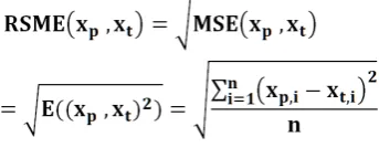
4.1. Root mean squared error

Mean squared error (MSE), is a predictive regression model that is a different way to quantify the distinction between set of actual (target) values, xt and set of predicted values, xp. The root mean squared error (RMSE) is defined as: the mean absolute error averages of each error neglecting its sign. Mean-squared error tends to exaggerate the effect of outliers, but absolute error does not have this performance. All error values are treated evenly according to their magnitude.

4.2. The correlation coefficient

The correlation coefficient is a measure of how trends in actual values are followed by trends in the predicted ones. It is an evaluation of how well the

predicted values from a predicted model fit the real-life data. The correlation coefficient is a magnitude in the range of -1 and 1. If the predicted and actual values are independent and no correlation exists between them, the correlation coefficient is close to zero. If the strength of the relationship between the actual and predicted values increases, so does the correlation coefficient. An ideal fit gives a coefficient equal to unity. Opposite but correlated trends result in a correlation coefficient magnitude limit to -1. Negative correlation values are not typically expected in the learning of a predictive model.

5. RESULTS AND DISCUSSION

5.1. Error analysis

The experimental data used for training the models is taken from Bowen et al. [33]. The error analysis for different methods is listed in Tables 1-3. Table 1 shows the analysis of correlation coefficient for various methods. An ideal value for correlation coefficient is equal to 1. Closer to unity, values show better agreement between predicted and experimental data and closer to zero is an indication of less agreement between them. According to Table 1, the best value of correlation coefficient for this data set is obtained from KNN method. Other methods also indicate good prediction and

negligible errors.

189

Table 3 represents the results of root mean squared error for various methods based on the selected data set. Root mean squared error is the rejection like mean absolute error and the ideal value for this error is zero. KNN method has the best prediction for this dataset according to this error and the results are shown in Table 2.

33. Bowen, W., Jones, M. Welfoot, J. Yousef, H. (2000) Predicting salt rejections at nanofiltration membranes using artificial

neural networks, Desalination 129, 147–162.

Figure 1. KNN predictions for pH=4.

0 10 20 30 40 50 60 70 80 90 100

0 0.5 1 1.5 2 2.5 3

R ej ec tio n ( % ) Pressure (bar) 0.001M(Exp) 0.01M(Exp) .01M(Perdiction)

Table 1: The analysis of correlation coefficient

Method Least Med Sq. SMOreg _PerceptronMultilayer IBK M5P Regression By _{Discretization} Correlation

Coefficient 0.8900 0.9100 0.9620 0.9655 0.9600 0.9400

Table 2:The analysis of Mean Absolute Error

Method Least Med Sq. SMOreg _PerceptronMultilayer IBK M5P Regression By _{Discretization}

Mean Absolute

Error 8.67 7.91 5.82 4.65 5.11 5.56

Table 3: The analysis of Root Mean Squared Error.

Method Least Med Sq. SMOreg _PerceptronMultilayer IBK M5P Regression By _{Discretization}

Root Mean Squared

Error 11.83 9.79 7.12 6.06 6.37 7.30

Figure 2. KNN predictions for pH=6.25

Figure 3. KNN predictions for pH=9

50 55 60 65 70 75 80 85 90 95

0 0.5 1 1.5 2 2.5 3

R ej ec tio n ( % ) Pressure (bar)

0.003 M (Exp) 0.01 M (Exp) .01 M (perdiction)

20 30 40 50 60 70 80 90 100

0 0.5 1 1.5 2 2.5 3

R ej ec tio n ( % ) Pressure (bar)

0.01 M (Exp) 0.1 M (Exp) 0.1 M (perdiction)

Figure 2. KNN predictions for pH=6.25

Figure 3. KNN predictions for pH=9

50 55 60 65 70 75 80 85 90 95

0 0.5 1 1.5 2 2.5 3

R ej ec tio n ( % ) Pressure (bar)

0.003 M (Exp) 0.01 M (Exp) .01 M (perdiction)

20 30 40 50 60 70 80 90 100

0 0.5 1 1.5 2 2.5 3

R ej ec tio n ( % ) Pressure (bar)

0.01 M (Exp) 0.1 M (Exp) 0.1 M (perdiction)

Figure 3: KNN predictions for pH=9 Figure 1: KNN predictions for pH=4

Figure 2: KNN predictions for pH=6.25

Figures 1 to 3 illustrate the results predicted for the rejection as a function of the concentration and pH based on the KNN model. The KNN model is able to account for the nanofiltration rejection at low and high concentrations. The KNN model also accounts very well for the change of pH. The predicted values were calculated at several pHs to ensure that the model was able to predict well using experimental data. In addition, training was performed by using the experimental data and the model was validated for some experimental data obtained at this range [33]. It must be noted that R is the experimental and R’ is the predicted rejection.

6. CONCLUSIONS

Rejection is investigated statistically as an index of membrane separation efficiency. The results show that rejection increases with an increase in pressure. At higher concentrations, nanofiltration rejections are lower than that of lower concentrations, since the membrane has a limited capacity for ion separation.

190

Machine Learning methods have been used for predicting the value of the rejection in nanofiltration. This application is important because the ability for correct predictions can help to select the best model.

REFERENCES

1. Hilal, N., Al-Zoubi, H., Darwish, N.A., Mohammad, A.W., AbuArabi, M., a comprehensive review of Nanofiltration membranes: treatment, pretreatment, modeling, and atomic force microscopy, Desalination, Vol. 170, (2004), pp. 281–308.

2. Ho, W. S., Sirkar, K. K. (1992) Membrane Handbook; Chapman & Hall: New York.

3. Schafer, A. I. Fane, A. G., Waite, T. D. (2005) Nanofiltration: Principles and Applications; Elsevier: New York.

4. Lonsdale, H. K., J. Membr. Sci, Vol. 10, (1982), pp. 81-181.

5. Spiegler, K., Kedem, O., Thermodynamics of hyper-filtration (reverse osmosis): criteria for efficient membranes, Desalination, Vol. 1, (1966), pp. 311–326. 6. Xu, X., Spencer, H. G., Desalination, Vol. 114,

(1997), pp. 129-137.

7. Perry, M., Linder, C., Desalination, Vol. 71, (1989), p. 233.

8. Williams, M. (2003) Tech. rep., Williams Engineering Services Company Inc.

9. Morrison, F. A. Jr., Osterle, J.F., Journal of Chemical Physics, Vol. 43, (1965), p. 2111.

10. Gross, R. J., Osterele, J. F., Journal of Chemical Physics, Vol. 49, No. 228, (1968), p. 19.

11. Fair, J. C., Osterele, J. F., Journal of Chemical Physics, Vol. 54, (1971), p. 3307.

12. Diez, M., Martinez Villa, L., Hernandez Gimenez, F., Tajerina Garcia, F., Journal of Colloid Interface Science, Vol. 132, No. 27, (1989), p. 293.

13. Sasidhar, V., Ruckenstien, E., Electrolyte osmosis through capillaries, Journal of Colloid Interface Science, Vol. 82, (1981), p. 439.

14. Sasidhar, V., Ruckenstien, E., Journal of Colloid Interface Science, Vol. 85, (1982), p. 332.

15. Neogi, P., Ruckenstein, E., Journal of Colloid Interface Science, Vol. 79, (1981), p. 159.

16. Probstein, R.F., Sonin, A.A., Yung, D., Desalination, Vol. 13, (1973), p. 303.

17. Wang, X., Tsuru, T., Nakao, Sh., Kimura, Sh., Journal of Membrane Science Vol. 103, (1995), pp. 117-133. 18. Smit, J. A. M., Journal of Colloid and Interface

Science, Vol. 132, (1989), p. 413.

19. Hijnen, H. J. M., Van Daalen, J., Smit, J. A. M. J. Colloid Interface Sci,Vol. 107, (1985), p. 525. 20. Smit, J. A. M., Colloid and Interface Science, Vol.

132, (1989), pp. 413-424.

21. Tsuru, T., Nakao, S., Kimura, S. J. Chem. Eng. Japan, Vol. 24, (1991), pp. 511–517.

22. Nasseh, V. Chemical Engineering Science, Vol. 53, (1998), pp. 1253-1265.

23. Giddings, J. C. (1991) Unified Separation Science, New York, Wiley.

24. Scarpello, J. T., Nair, D. F. dos Santos, L. M., White, L. S., Livingston, A. G. J. Membr. Sci., Vol. 203, (2002), pp. 71–85.

25. Zwijnenberg, H. J., Krosse, A. M., Ebert, K., Peinemann, K. V., Cuperus, JAOCS. American Oil Chemists’ Society, Vol. 76, (1999), pp. 83-87. 26. Brinkman, H. C. Appli. Sci. Res, A1, (1947), pp.

27–34.

27. Al-Zoubi, H., Hilala, N. Darwish, N.A., Mohammad, A.W. Rejection and modeling of sulphate and potassium salts by nanofiltration membranes: neural network and Spiegler–Kedem model, Desalination, Vol. 206, (2007), pp. 42–60.

28. Rousseeuw, P. J., Leroy, A. M. (1987) Robust Regression and Outlier Detection, Wiley, New York. 29. Shevade, S. K., Keerthi, S. S., Bhattacharyya, C.,

Murthy, K.R.K. (1999) Improvements to the SMO Algorithm for SVM Regression, IEEE Transactions on Neural Networks.

30. Ykin, S. H. (1999) Neural Networks: A

Comprehensive Foundation, Prentice Hall, London. 31. Wang, Y., Witten, I. H. (1997) Introduction of model

trees for predicting continuous classes, 9th European Conference on Machine Learning.

32. Breiman, L., Friedman, J. H., Olshen, R.A., Stone, C. J. (1984) Classification and Regression Trees, Wadsworth, Belmont CA.

33. Bowen, W., Jones, M. Welfoot, J. Yousef, H. Predicting salt rejections at nanofiltration membranes using artificial neural networks, Desalination, Vol. 129, (2000), pp. 147–162.