www.ijaems.com Page | 175
Study of Pruning Techniques to Predict Efficient
Business Decisions for a Shopping Mall
Jayesh Ambekar
1, Mohit Berika
2, Sarang Ambotkar
3, Sachin Desai
41,2,3Student, Smt. Indira Gandhi College of Engineering, Koparkhairane, Navi Mumbai, India 4Assitant Professor, Smt. Indira Gandhi College of Engineering, Koparkhairane, Navi Mumbai, India
Abstract— The shopping mall domain is a dynamic and
unpredictable environment. Traditional techniques such as fundamental and technical analysis can provide investors with some tools for managing their shops and predicting their business growth. However, these techniques cannot discover all the possible relations between business growth and thus, there is a need for a different approach that will provide a deeper kind of analysis. Data mining can be used extensively in the shopping malls and help to increase business growth. Therefore, there is a need to find a perfect solution or an algorithm to work with this kind of environment. So we are going to study few methods of pruning with decision tree. Finally, we prove and make use of the Cost based pruning method to obtain an objective evaluation of the tendency to over prune or under prune observed in each method.
Keywords— Cost based pruning, Data Mining, Itemsets, Pruning.
I. INTRODUCTION
A. Shopping Mall
In today’s world, people often refer to visit the shopping mall for shopping where they get what they need in one place instead of visiting local shops one by one. Hence, this brings the mall authority a huge burden which has to deal with major issues like managing the data for each and every product, attracting the customers towards mall by predicting their needs, and decisions to increase the growth of each shop.
B. Decision Tree pruning
Decision tree builds classification or regression models in the form of a tree structure. It breaks down a dataset into smaller and smaller subsets while at the same time an associated decision tree is incrementally developed. The final result is a tree with decision nodes and leaf nodes. A decision node (e.g., Outlook) has two or more branches (e.g., Sunny, Overcast and Rainy). Leaf node (e.g., Play) represents a classification or decision. The topmost decision node in a tree which corresponds to the best predictor called root node. Decision trees can handle both categorical and numerical data. There are several major decision tree pruning techniques. They are:
1 .Post-pruning 2. Pre-pruning.
II. APPROACHES
1. Post pruning:
The important step of tree pruning is to define a criterion be used to determine the correct final tree size using one of the following methods:
1. Use a distinct dataset from the training set (called validation set), to evaluate the effect of post-pruning nodes from the tree.
2. Build the tree by using the training set, then apply a statistical test to estimate whether pruning or expanding a particular node is likely to produce an improvement beyond the training set.
o Error estimation
o Significance testing (e.g., Chi-square test)
3. Minimum Description Length principle : Use an explicit measure of the complexity for encoding the training set and the decision tree, stopping growth of the tree when this encoding size (size(tree) + size(misclassifications(tree)) is minimized.
The first method is the most common approach. In this approach, the available data are separated into two sets of examples: a training set, which is used to build the decision tree, and a validation set, which is used to evaluate the impact of pruning the tree. The second method is also a common approach. Here, we explain the error estimation and Chi2 test.
www.ijaems.com Page | 176 In the following example we set Z to 0.69 which is equal
to a confidence level of 75%.
The error rate at the parent node is 0.46 and since the error rate for its children (0.51) increases with the split, we do not want to keep the children.
• Post-pruning using Chi2 test:
In Chi2 test we construct the corresponding frequency table and calculate the Chi2 value and its probability.
If we require that the probability has to be less than a limit (e.g., 0.05), therefore we decide not to split the node.
• Cost based pruning:
This is one of the post pruning technique. In this method not only an error rate is considered at each node but also a cost is considered. That is for pruning decision tree error rate and cost of deciding selection of one or more class-label attribute is considered. Here one example is explained for healthy or sick classification. Two type of pruning is shown error pruning and cost based pruning:
1. Pre-pruning:
Pre-pruning is also called forward pruning or online-pruning. It prevents the generation of non-significant branches. Based on statistical significance test we can tree generation will be stopped when there is no statistically significant association between any attribute and the class at a particular node. In pre pruning, we decide during the building process when to stop adding attributes (possibly based on their information gain). However, this may be problematic because sometimes attributes individually do not contribute much to a decision,
but when two or attributes are combined, they may have a significant impact on the decision tree.
• Cost-Sensitive Decision Trees with Pre-pruning:
The algorithms we proposed in this paper are based on [13], incorporating two simple pre-pruning methods, described below. 2-Level Tree. With this approach, we just build the tree with no more than 2 levels. [18] and [19] have used similar approaches for error-based tree building, and shown that simpler trees often work quite well in many data sets. In this paper, we use the same idea in the cost-sensitive tree building process. The 1 [13]’s work includes both misclassification costs and attribute costs. Attribute costs can act as a natural pruning mechanism, because an expensive attribute is unlikely to be chosen to split the data further, unless there is a large gain in the reduction of the misclassification cost. Nevertheless, over-fitting could still happen, especially when the attribute cost is small or zero (as we study here).
Threshold Pruning Tree: Another common approach for pre-pruning is imposing a pre-specified threshold on the splitting measure. Using cost reduction alone, the unpruned tree [13] would be expanded until the cost reduction is smaller than or equal to 0. We set a threshold on the cost reduction to avoid over-fitting. We assume that the tree expansion is worthwhile only when the cost reduction is greater than the sum of False Positive(FP) and False Negative(FN) cost (we assume that the cost of True Positive and True Negative is 0). That is: Threshold = F P + F N For cost-sensitive trees with both pre-pruning methods, the following is used to label leaves. If the cost reduction is 0 or negative (for the 2-level trees), or if the cost reduction is less than the threshold (pre-specified threshold pruning), a leaf node is formed, and it should be labeled as the class minimizing the expected cost according to train data falling into the node. If no instance is falling into a node, then a leaf is also formed labelled as the class minimizing the expected cost of its parent node.
Chi-square pruning
www.ijaems.com Page | 177 features already branched on before this node. This
is the hypothesis that we form to determine whether or not to reject the split. The split is only accepted if this null hypothesis can be rejected with high probability. We can perform chi-squared test as:
According to this equation one contingency table is generated and according to this values .
Consider one example, The statistical for Pearson’s chi-square test [19], which will be used here as a test of independence. To think about this, suppose that at the current node the data is split 10:10 between negative and positive examples. Further more, suppose there are 8 instances for which Xk is false, and 12 for which Xk is true. We’d like to understand whether a split that generates labeled data 3:5 (on the Xk false branch) and 7:5 (on the Xk true branch) could occur simply by chance.
III. ATTRIBUTE SELECTION MEASURES
Attribute selection is the process of removing the redundant attributes that are deemed irrelevant to the data mining task. The objective of attribute selection is therefore to search for a worthy set of attributes that produce comparable classification results to the case when all the attributes are used. Measures for selecting the best split attributes are almost all defined in terms of the reduction of impurity from parent to child node(before splitting)[13]. The larger the reduction of impurity; the better the selected split attribute. There are number of attribute selection measures which exist. Let t, be a training set of class labeled tuples. Suppose the class label has c distinct values defining c distinct classes.
3.1.1 Information Gain
Information gain measures the expected reduction in entropy caused by partitioning the examples according to attribute.ID3 uses information gain as its attribute selection measure. This is based on Shannon’s entropy.
Where Info(D) is also known as entropy of D. 3.1.2 Gain Ratio
Information gain measure is biased toward tests with many outcomes. Therefore the information gained by partitioning on attribute is maximal, such a partitioning is useless for classification.C4.5, a successor of ID3 [2] uses an extension to the information gain known as Gain ratio.
Where Gain(A) is expected reduction in the information requirement caused by knowing the value of A(attribute).
SplitInfo(A) is value defined analogously with Info(D) as
3.1.3 Gini Index
Gini index is used in Classification and Regression Tree also knowm as CART. Gini index measures the impurity of D, a data partition or set of training tuples as
where Pi is the probability that a tuple in D belongs to the class Ci.
IV. PARAMETERS IN DECISION TREE
PRUNING ALGORITHM A. Over fitting
Over fitting is a significant practical difficulty for decision tree models and many other predictive models. Over fitting happens when the learning algorithm continues to develop hypotheses that reduce training set error at the cost of an increased test set error. There are several approaches to avoiding over fitting in building decision trees. The possibility of over fitting exists because the criterion used for training the model is not the same as the criterion used to judge the efficacy of a model. In particular, a model is typically trained by maximizing its performance on some set of training data. However, its efficacy is determined not by its performance on the training data but by its ability to perform well on unseen data. Over-fitting occurs when a model begins to "memorize" training data rather than "learning" to generalize from trend. As an extreme example, if the number of parameters is the same as or greater than the number of observations, a simple model or learning process can perfectly predict the training data simply by memorizing the training data in its entirety, but such a model will typically fail drastically when making predictions about new or unseen data, since the simple model has not learned to generalize at all.
www.ijaems.com Page | 178 Even when the fitted model does not have an excessive
number of parameters, it is to be expected that the fitted relationship will appear to perform less well on a new data set than on the data set used for fitting. In particular, the value of the coefficient of determination will shrink relative to the original training data.
In order to avoid over-fitting, it is necessary to use additional techniques (e.g. cross-validation, regularization, early stopping, pruning, Bayesian priors on parameters or model comparison), that can indicate when further training is not resulting in better generalization. The basis of some techniques is either (1) to explicitly penalize overly complex models, or (2) to test the model's ability to generalize by evaluating its performance on a set of data not used for training, which is assumed to approximate the typical unseen data that a model will encounter.
How to avoid Over-fitting:
To avoid over-fitting add the regularization if there are many features. Regularization forces the magnitudes of the parameters to be smaller (shrinking the hypothesis space). For this add a new term to the cost function
which penalizes the magnitudes of the parameters like as
B. Under-fitting:
If our algorithm works badly with points in our data set, then the algorithm under-fitting the data set. It can be checked easily through the cost function measures. Cost function in linear regression is half the mean squared error ex. if mean squared error is c the cost function is 0.5C 2. If in an experiment cost ends up high even after many iterations, then chances are we have an under-fitting problem. We can say that learning algorithm is not good for the problem. Under-fitting is also known as high bias (strong bias towards its hypothesis). In other words we can say that hypothesis space the learning algorithm explores is too small to properly represent the data.
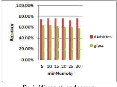
V. EXPERIMENTS & RESULTS
In this section illustrates some experiments on data set in Weka. There are two data sets, Diabetes & Glass. In Diabetes dataset there are 768 instances and 9 attributes. In Glass dataset there are 214 instances and 10 attributes. Here weka 3.7.7 is used for experiments. In weka there are some pruning factors like minNumobj, numFold etc. minNumobj in weka specifies minimum no of objects(instances) at the leaf node. That is when decision tree is induced, at every split it will check minimum no of object at leaf. If instances at leaf are greater than minimum num of obj then pruning is done. NumFold parameter in weka is affected only when reduced error pruning parameter is true. That is this
parameter determines amount of data used for reduced error pruning. Among numFolds one fold is used for pruning and rest of them for growing the tree. Suppose numFold is 3 then 1 fold is used for pruning and 2 fold for training for growing the tree.
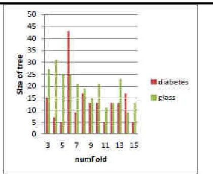
Experiments on weka show the accuracy and size of tree for particular parameter. Here size of tree is considered because it is mainly concerned with pruning. It indicates with pruning how accuracy (increasing or decreasing) is get. Below graph shows measure for accuracy and size of tree for both data sets in weka.
Fig 3: Minnumobj vs Accuracy
Fig 3 and Fig 4 shows comparision of both data sets for the accuracy & size of tree when minNumobj parameter is used. Whenever minnumobj is increased the accuracy becomes almost same but tree size is changed. At starting it seems to be increasing, but as minnumobj is increased repeatedly, the size of tree is decreased which means more pruning is done and accuracy is almost same.
Fig 4: Minnumobj vs Size of tree
www.ijaems.com Page | 179 Fig 6: Num of folds vs Size if tree
Fig 5 and Fig 6 shows comparision of accuracy and size of tree for both data set when numFold parameter is used. For reduced error pruning numFold is used. Whenever numfolds are increased the accuracy for both datasets almost increases, but here it can’t be perfect for size of the tree. Dataset size of the diabetes tree suddenly increases for values ranging 5 to 6. For Glass dataset it is almost increases at starting, but as the numfolds is increased,the size of tree reduces and but the accuracy is almost same.
VI. FUTURE WORK
As a direction of future work, we are implementing a web application with an improved GUI. The web Application created will be website created will have login facility for users. It will have section for the users to access details of the products. The output will consists of the list of real time analysis of the products. The other way to get the accurate result is by making the system analyze the products manually, we are investigating the effect of choosing the appropriate algorithms to implement analysis on products. This technique can be further used in predicting the more complex environments.
VII. CONCLUSION
In the Research work we have thus studied the existing system for data mining consisting of the Apriori algorithm along with its advantages and disadvantages. Furthermore we have studied the cost based pruning algorithm is efficient for pruning large dataset. Execution time and pruned cost based data are the main performance factors of this work. From the experimental results, we observed that, the Pruning algorithm required minimum execution time and it also identified more number of frequent items. Mining techniques will then be very significant in order to conduct advanced analysis, such as determining trends and finding interesting patterns, on streaming data using pruning techniques in data mining.
REFERENCES
[1] Erwin, R.P. Gopalan and N.R. Achuthan "Efficient Mining of High Utility Itemsets from Large Data Sets", Proc. 12th Pacific-Asia Conf. Advances in Knowledge Discovery and Data Mining (PAKDD), pp.554 -561
[2] Shou-Hsiung Cheng, ―Forecasting the Change of Intraday Stock Price by Using Text Mining News of Stock‖, IEEE, 2010.
[3] Pablo Carballeira, Juli´an Cabrera, Fernando Jaureguizar, and Narciso Garc´ıa Grupo de Tratamiento de Im´agenes “AN OPTIMAL YET FAST PRUNING ALGORITHM TO REDUCE LATENCY IN MULTIVIEW PREDICTION STRUCTURES”, ETSI de Telecomunicaci´on, Universidad Polit´ecnica de Madrid, Ciudad Universitaria, 28040, Madrid, Spain. [4] Floriana Esposito, Member, IEEE, Donato Malerba,
Member, IEEE, and Giovanni Semeraro, Member, IEEE “A Comparative Analysis of Methods for Pruning Decision Trees” IEEE TRANSACTIONS ON PATTERN ANALYSIS AND MACHINE INTELLIGENCE, VOL. 19, NO. 5, MAY 1997 [5] Ling, C., Yang, Q., Wang, J., Zhang, S.: Decision trees
with minimal costs. In: Proceedings of the 21st International Conference on Machine Learning. (2004) [6] Holte, R.: Very simple classification rules perform well
on most commonly used datasets. Machine Learning 11 (1993) 63–91