ISSN 2322-5149 ©2014 JNAS
The study of energy conservation in wireless
sensor networks
Javad Hamidzadeh
1*and Saeed Rakhshanipoor
21- Department of Computer Engineering, Sadjad University of Technology, Mashhad, Iran
2- MSC student, Department of Computer engineering, Ferdous Branch, Islamic Azad University, Ferdous, Iran
Corresponding author:
Javad Hamidzadeh
ABSTRACT: In recent years, wireless sensor networks (WSNs) used for environmental monitoring, health monitoring and industrial monitoring has been widely recommended as a means of reducing the energy consumption and CO2 emissions. Wireless sensing in commercial and office buildings has lead to a greater awareness of the condition of buildings and their systems: As it provides information necessary for those in charge of building operation and maintenance to recognize limits and non-functioning equipment and systems and prioritise building maintenance tasks etc. In the recent years, numerous articles have been published describing new algorithms, routing protocols and architectures aiming at WSN lifetime maximization, through energy awareness. Already proposed routing techniques for WSNs aiming at energy conservation, employ routing tactics such as data aggregation, in-network processing, clustering, different node role assignment and data-centric methods. Duty cycling is mainly focused on the networking subsystem. The most effective energy-conserving operation is putting the radio transceiver in the (low-power) sleep mode whenever communication is not required. Ideally, the radio should be switched off as soon as there is no more data to send/receive, and should be resumed as soon as a new data packet becomes ready.
Keywords: benefits, cluster heads, topology control, data driven.
INTRODUCTION
Wireless sensor networks (WSNs)
1182
The main benefits of wireless sensor networks
Wireless sensing in commercial and office buildings has lead to a greater awareness of the condition of buildings and their systems: As it provides information necessary for those in charge of building operation and maintenance to recognise limits and non-functioning equipment and systems and prioritise building maintenance tasks etc. based on costs and other important factors (Brambley , 2005, Menzel , 2008). The main benefits of this are: An increased lifespan for equipment/electric appliances; An improved building environment for occupants; The ability to detect impending faults and therefore minimise energy usage associated with facility assets and increase reliability while reducing costs; Economies of scale gained from monitoring, tracking and responding to the status of multiple building assets from centralised or regional locations; Lower energy and operating costs leading to an advantageous return on investment. For example energy management systems based on WSNs can save an average of 10 % in overall building energy consumption and the energy savings can be as high as 30% depending on occupancy (Lun-Wu Yeh , 2009).
Definition of clusters
The previous Section 10.3 has introduced a hierarchy into a network by designating some nodes asbelonging to a backbone, a dominating set. Another idea for a hierarchy is to locally mark somenodes as having a special role, for example, controlling neighboring nodes. In this sense, local groups or clusters of nodes can be formed; the “controllers” of such groups are often referred toas clusterheads. The hoped-for advantages of such clustering are similar to that of a backbone, butwith additional emphasis on local resource arbitration (e.g. in MAC protocols), shielding higherlayers of dynamics in the network (making routing tables more stable since all traffic is routed over the clusterheads), and making higher-layer protocols more scalable (since the size and complexity ofthe network as seen by higher layers is in a sense reduced by clustering). In addition, clusterheadsare natural places to aggregate and compress traffic converging from many sensors to a singlestation.
Routing techniques
In the recent years, numerous articles have been published describing new algorithms, routing protocols and architectures aiming at WSN lifetime maximization, through energy awareness. Already proposed routing techniques (Akkaya and younis, 2002; Alkaraki and kamal, 2004) for WSNs aiming at energy conservation, employ routing tactics such as data aggregation, in-network processing, clustering, different node role assignment and data-centric methods. There are several ways of categorizing these protocols and algorithms. For example, they can be discriminated depending on the network structure to Flat Networks Routing (Data-centric routing (Akkaya and younis, 2002), Hierarchical Networks Routing and Locationbased Routing (Alkaraki and kamal, 2004). Intanagonwiwat . (2000) proposed directed diffusion a data-centric (i.e. all communication is for named-data) and application-aware paradigm aiming at avoiding unnecessary operations of network layer routing in order to save energy by selecting empirically good paths and by caching and processing data within the network. Yao and Gehrke (2002) proposed another data-centric protocol, namely, COUGAR, for an architecture which treats the network as a huge distributed database system. Energy Aware Routing, a protocol proposed by Shah and Rabaey (2002), although similar to directed diffusion, it differs in the sense that it uses occasionally sub-optimal paths to obtain energy benefits. This protocol can achieve longer network lifetime as energy is dissipated more equally among all nodes. TEEN and APTEEN, two hierarchical routing protocols are proposed by Manjeshwar and Agarwal (2001). TEEN (Threshold-sensitive Energy Efficient sensor Network protocol) and APTEEN (Adaptive Periodic Threshold-(Threshold-sensitive Energy Efficient sensor Network protocol) are suitable for time-critical applications. In both protocols the key factor is the measured attribute’s value. The additional feature of APTEEN is the capability of changing the periodicity and the parameters of TEEN according to user and application needs. The concept of generic, utility-based decision making in WSN is described in (Byers and Nasser, 2000), where Byers and Nasser try to quantify the cost of each action performed by a sensor, by adopting heuristic assessments. Apart from routing protocols, PowerTOSSIM (Shrayder ., 2004), a WSN simulation tool has been developed. PowerTOSSIM provides an accurate, per-node estimate of power consumption. PowerTOSSIM is an extension of TOSSIM (Levis ., 2003; Sridharam ., 2009; Levis and Lee., 2006) the event-driven simulation for applications.
Types of sensor networks
1183
an ad hoc or in a pre-planned manner. In ad hoc deployment, sensor nodes can be dropped from a plane and randomly placed into the target area. In pre-planned deployment, there is grid placement, optimal placement (Toumpis and Tassiulas, 2006) 2-d and 3-d placement (Yick ., 2006; Pompili ., 2006) models. In a terrestrial WSN, reliable communication in a dense environment is very important. Terrestrial sensor nodes must be able to effectively communicate data back to the base station. While battery power is limited and may not be rechargeable, terrestrial sensor nodes however can be equipped with a secondary power source such as solar cells. In any case, it is important for sensor nodes to conserve energy. For a terrestrial WSN, energy can be conserved with multi-hop optimal routing, short transmission range, in-network data aggregation, eliminating data redundancy, minimizing delays, and using low duty-cycle operations. Underground WSNs (Akyildiz and Stuntebeck 2006; Li and Liuconsist, 2007) of a number of sensor nodes buried underground or in a cave or mine used to monitor underground conditions.Figure 1. A medical sensor network application
Additional sink nodes are located above ground to relay information from the sensor nodes to the base station. An underground WSN is more expensive than a terrestrial WSN in terms of equipment, deployment, and maintenance. Underground sensor nodes are expensive because appropriate equipment parts must be selected to ensure reliable communication through soil, rocks, water, and other mineral contents.
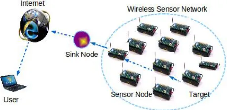
Figure 2. Illustration of Wireless Sensor Networks
1184
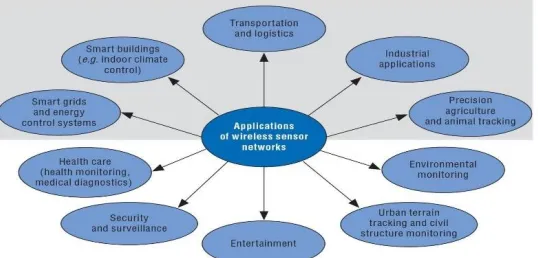
Figure 3. Application of wireless sensor networks
Autonomous underwater vehicles are used for exploration or gathering data from sensor nodes. Compared to a dense deployment of sensor nodes in a terrestrial WSN, a sparse deployment of sensor nodes is placed underwater. Typical underwater wireless communications are established through transmission of acoustic waves. A challenge in underwater acoustic communication is the limited bandwidth, long propagation delay, and signal fading issue. Another challenge is sensor node failure due to environmental conditions. Underwater sensor nodes must be able to self-configure and adapt to harsh ocean environment. Underwater sensor nodes are equipped with a limited battery which cannot be replaced or recharged. The issue of energy conservation for underwater WSNs involves developing efficient underwater communication and networking techniques. Multi-media WSNs (Akyildiz ., 2007) have been proposed to enable monitoring and tracking of events in the form of multimedia such as video, audio, and imaging. Multi-media WSNs consist of a number of low cost sensor nodes equipped with cameras and microphones. These sensor nodes interconnect with each other over a wireless connection for data retrieval, process, correlation, and compression. Multi-media sensor nodes are deployed in a pre-planned manner into the environment to guarantee coverage. Challenges in multi-media WSN include high bandwidth demand, high energy consumption, quality of service (QoS) provisioning, data processing and compressing techniques, and cross-layer design. Multi-media content such as a video stream requires high bandwidth in order for the content to be delivered. As a result, high data rate leads to high energy consumption. Transmission techniques that support high bandwidth and low energy consumption have to be developed. QoS provisioning is a challenging task in a multi-media WSN due to the variable delay and variable channel capacity. It is important that a certain level of QoS must be achieved for reliable content delivery. In-network processing, filtering, and compression can significantly improve network performance in terms of filtering and extracting redundant information and merging contents. Similarly, cross-layer interaction among the layers can improve the processing and the delivery process. Mobile WSNs consist of a collection of sensor nodes that can move on their own and interact with the physical environment. Mobile nodes have the ability sense, compute, and communicate like static nodes. A key difference is mobile nodes have the ability to reposition and organize itself in the network. A mobile WSN can start off with some initial deployment and nodes can then spread out to gather information. Information gathered by a mobile node can be communicated to another mobile node when they are within range of each other. Another key difference is data distribution. In a static WSN, data can be distributed using fixed routing or flooding while dynamic routing is used in a mobile WSN. Challenges in mobile WSN include deployment, localization, self-organization, navigation and control, coverage, energy, maintenance, and data process. Mobile WSN applications include but are not limited to environment monitoring, target tracking, search and rescue, and real-time monitoring of hazardous material.
1185
For environmental monitoring in disaster areas, manual deployment might not be possible. With mobile sensor nodes, they can move to areas of events after deployment to provide the required coverage. In military surveillance and tracking, mobile sensor nodes can collaborate and make decisions based on the target. Mobile sensor nodes can achieve a higher degree of coverage and connectivity compared to static sensor nodes. In the presence of obstacles in the field, mobile sensor nodes can plan ahead and move appropriately to obstructed regions to increase target exposure.The differences between sensor networks and ad hoc networks
Realization of these and other sensor network applications require wireless ad hoc networking techniques. Although many protocols and algorithms have been proposed for traditional wireless ad hoc networks, they are not well suited for the unique features and application requirements of sensor networks. To illustrate this point, the differences between sensor networks and ad hoc networks are outlined below (Perkins, 2000):
The number of sensor nodes in a sensor network can be several orders of magnitude higher than the nodes in an ad hoc network.
Sensor nodes are densely deployed. Sensor nodes are prone to failures.
The topology of a sensor network changes very frequently.
Sensor nodes mainly use broadcast communication paradigm whereas most ad hoc networks are based on point-to-point communications.
Sensor nodes are limited in power, computational capacities, and memory.
Sensor nodes may not have global identification (ID) because of the large amount of overhead and large number of sensors (Perkins, 2000).
Figure 5. Target tracking in wireless sensor networks
Prolonging the Lifetime of Wireless Sensor Networks by Cross-Layer Interaction
A cross-layered approach for networking in Wireless Sensor Networks can be found in (Hoesel, ., 2004). According to this approach, a self-organizing MAC (Medium Access Control) protocol makes use of an algorithm of a sensor node intending to create a connected network based on local information only, and an integrated, efficient routing protocol. Operation here is entirely distributed and localized. Network lifetime is used as the metric to make the evaluation of the performance of the cross-layer optimized protocols. It measures the amount of time before a certain number of sensor nodes run out of battery power. It is proved that this scheme prolongs the lifetime of the network significantly in the mobile sensor scenario. The lifetime of this scenario is at least three times better than those of DSR and S-MAC. We must notice here that the lifetime in S-MAC and DSR is almost independent of message frequency. The explication of this fact is that the nodes use their receiver anyhow during the time interval they are awake. S-MAC and DSR protocols perform better in the static case than in the mobile one, in contrast to this protocol. The reason is that in the static scenario, routes need be established only once, while in the mobile scenario they have to be updated regularly (Hoesel, 2004).
Connecting clusters
1186
clusterheads that are at most three hopsaway. While for some networks, this might mean more connections than necessary, but there arenetworks where all this links are needed to ensure connectivity.In addition to this basic connectivity consideration, other aspects like load balancing betweenmultiple gateways can be considered. Various approaches have been proposed here; reference [53],for example, treats this topic in more detail.The challenge of wireless sensor networks
The constraints of sensor nodes render the design and management of a WSN very challenging. Firstly, sensors have limited resources such as battery lifetime (varying from hours to several years depending on the application), computational power, data storage and communication bandwidth. Hence, it is important for a WSN architecture to take into consideration the network topology, power consumption, data rate and fault tolerance in order to avoid significant energy consumption and improve bandwidth utilization (Akyildiz, 2002).
Sensing coverage
Sensing coverage characterizes the monitoring quality provided by a sensor network in a designated region. Different applications require different degrees of sensing coverage. While some applications may only require that every location in a region be monitored by one node, other applications require significantly higher degrees of coverage. For example, distributed detection based on data fusion (Varshney 1996) requires that every location be monitored by multiple nodes, and distributed tracking and classification (Li . 2002) requires even higher degrees of coverage. The coverage requirement for a sensor network also depends on the number of faults that must be tolerated. A network with a higher degree of coverage can maintain acceptable coverage in face of higher rates of node failures. The coverage requirement may also change after a network has been deployed, for instance, due to changes in application modes or environmental conditions. For example, a surveillance sensor network may initially maintain a low degree of coverage required for distributed detection. After an intruder is detected, however, the region in the vicinity of the intruder must reconfigure itself to achieve a higher degree of coverage required for distributed tracking. Although achieving energy conservation by scheduling nodes to sleep is not a new approach, none of the existing protocols satisfy the complete set of requirements in sensor networks. First, most existing solutions have treated the problems of sensing coverage and network connectivity separately. The problem of sensing coverage has been investigated extensively. Several algorithms aim to find a close-to-optimal solution based on global information. Both Cerpa and Estrin (2002) and Meguerdichian and Potkonjak (2003) apply linear programming techniques to select the minimal set of active nodes for maintaining coverage. A more sophisticated coverage model is used to address exposure-based coverage problems in Meguerdichian . (2001a, 2001b). The problem of finding the minimal exposure path is addressed in Meguerdichian . (2001a). The maximal breach path and maximal support path in a sensor network are computed using Voronoi diagram and Delaunay Triangulation techniques in Meguerdichian . (2001b). In Couqueur . (2002), node deployment strategies were investigated to provide sufficient coverage for distributed detection. Due to requirements for scalability and fault-tolerance, localized algorithms are more suitable and robust for large-scale wireless sensor networks that operate in dynamic environments.
S-MAC
S-MAC (Sensor-MAC) is a distributed protocol, which gives the possibility to nodes to discover their neighbors and build sensor networks for communication without being obliged to have master nodes. There are no clusters or cluster heads here. The topology is flat. This solution, proposed by [Ye, W., . (2002)], focuses mainly on the major energy wastage sources while achieving good scalability and collision avoidance capability. The major energy wastage sources may be classified into overhearing, idle listening, collisions and control packet overhead [Hoesel, L. V., . (2004)].
Environmental applications of wireless sensor networks
1187
The reduction of energy consumption in wireless sensor networks
Clustering (2005, 2009) is one of the key approaches used in wireless sensor networks to save energy. The clustering isaffected by the transmission range and in turn affects the energy consumption in the network. Bolian ., (2007)established an energy consumption approach for clustered wireless sensor networks and solve the optimal transmissionrange problem. Using this approach, the total energyconsumption can be estimated beforehand based on the trafficpattern, energy model, and network deployment parameters.This technique presents an insight into the energyconsumption behavior in clustered wireless sensor networksand the relationship among major factors. The optimaltransmission range for energy consumption is a function of thetraffic load and the node density, but the effect of node density is very limited. The reduction of energy consumption (2008) in wireless sensor networks is challenging issue, and grid-based clustering and routing schemes is playing a vital role due to their simplicity and feasibility. Thus, determining the optimal grid size in order to minimize energy consumption and prolong network lifetime becomes an important problem during the network planning and dimensioning phase. The previous researches have used the average distances within a grid and between neighbor grids to calculate the average energy consumption, which largely underestimates the real value. In this paper, Yanyan ., (2010) proposed, analyzed and evaluated the energy consumption models in wireless sensor networks with probabilistic distance distributions. These techniques have been validated by numerical and simulation results, which shows that they can be used to optimize grid size and minimize energy consumption accurately. The author also uses these approaches to study variable-size grids, which can further improve the energy efficiency by balancing the relayed traffic in wireless sensor networks.
DPM (Dynamic Power Management)
A scheme, contributing to dynamic increase of the lifetime of the sensor network, is proposed by Sinha . [Sinha, A., and Chandrakasan, A., (2001)]. Once the system is designed, additional power savings can be obtained by using dynamic power management (DPM). The basic idea behind DPM is to turn off the devices when not needed and get them back when needed. The switching of a node, from one state to another, takes some finite time and resource. So we have to be very careful when using DPM to accomplish maximum life of a sensor node. We may achieve good savings in power with this turning off of the node. However, in many cases it may not be known beforehand when a particular device is needed. Stochastic analysis can be used to predict the future events. The DPM sensor model deals with switching of node state in a power efficient manner. All the components in a node can be in different states. In general, if we have a number of N components in a sensor node, each node’s sleep state corresponds to a particular combination of component power modes. Each sleep state is characterized by latency and power consumption. The deeper the sleep state, the lesser the power consumption, and more the latency. For example, if a processor is in idle state then memory should be in sleep state. This removes some combinations from the node states.
Duty cycling
Duty cycling is mainly focused on the networking subsystem. The most effective energy-conserving operation is putting the radio transceiver in the (low-power) sleep mode whenever communication is not required. Ideally, the radio should be switched off as soon as there is no more data to send/receive, and should be resumed as soon as a new data packet becomes ready. In this way nodes alternate between active and sleep periods depending on network activity. This behavior is usually referred to as duty cycling, and duty cycle is defined as the fraction of time nodes are active during their lifetime. As sensor nodes perform a cooperative task, they need to coordinate their sleep/wakeup times. A sleep/wakeup scheduling algorithm thus accompanies any duty cycling scheme. It is typically a distributed algorithm based on which sensor nodes decide when to transition from active to sleep, and back. It allows neighboring nodes to be active at the same time, thus making packet exchange feasible even when nodes operate with a low duty cycle (i.e., they sleep for most of the time).
Topology Control
1188
application needs, so as to allow network operations while minimizing the number of active nodes (and, hence, prolonging the network lifetime).Data Driven
Data prediction techniques build a model describing the sensed phenomenon, so that queries can be answered using the model instead of the actually sensed data. There are two instances of a model in the network, one residing at the sink and the other at source nodes (so that there are as many pairs of models as sources). The model at the sink can be used to answer queries without requiring any communication, thus reducing the energy consumption. Clearly, this operation can be performed only if the model is a valid representation of the phenomenon at a given instant. Here comes into play the model residing at source nodes, which is used to ensure the model effectiveness. To this end, sensor nodes just sample data as usual and compare the actual data against the prediction. If the sensed value falls within an application-dependent tolerance, then the model is considered valid. Otherwise, the source node may transmit the sampled data and/or start a model update procedure involving the sink as well. The features of a specific data prediction technique depend on the way the model is built. To this end, data prediction techniques can be split into three main classes.
MOBILITY-BASED ENERGY CONSERVATION SCHEMES
Mobility of sensor nodes is actually feasible, and it can be accomplished in different ways (Akyildiz and Kasimoglu., 2004). For example, sensors can be equipped with mobilizers for changing their location. As mobilizers are generally quite expensive from the energy consumption standpoint, adding mobility to sensor nodes may be not convenient. In fact, the resulting energy consumption may be greater than the energy gain due to mobility itself. So, instead of making each sensor node mobile, mobility can be limited to special nodes which are less energy constrained than the ordinary ones. In this case, mobility is strictly tied to the heterogeneity of sensor nodes. On the other side, instead of providing mobilizers, sensors can be placed on elements which are mobile of their own (e.g. animals, cars and so on). There are two different options in this case. First, all sensors are put onto mobile elements, so that all nodes in the network are mobile. Alternatively, only a limited number of special nodes can be placed on mobile elements, while the other sensors are stationary. Anyway, in both cases there is no additional energy consumption overhead due to mobility, but the mobility pattern of mobile elements has to be taken into account during the network design phase (more details are provided below). By introducing mobility in wireless sensor networks, several issues regarding connectivity can be afforded. First, during sensor network design, a sparse architecture may be considered as an option, when the application requirements may be satisfied all the same. In this case, it is not required to deploy a large number of nodes, as the constraint of connectivity isrelaxed because mobile elements can reach eventual isolated nodes in the network. A different situation happens when a network, assumed to be dense by design, actually turns out to be sparse after the deployment. For example, nodes involved in a random deployment might be not sufficient to cover a given area as expected, due to physical obstacles or damages during placement. In this context, solutions exploiting Unmanned Aircrafts as mobile collectors (Jenkins ., 2007; Venkitasubramaniam ., 2004) can be successfully used. In addition, an initially connected network can turn into a set of disconnected subnetworks due to hardware failures or energy depletion. In these cases, nodes can exploit mobility in order to remove partitions and re organize the network so that all nodes are connected again (Dini ., 2008). In this case, the sensor network lifetime can be extended as well.
REFERENCES
Agre J and Clare L. 2000. An integrated architecture for cooperative sensing networks, IEEE Computer Magazine (May 2000) 106–108.
Ahmed I. 2008. MugenPeng and Wenbo Wang, “Uniform Energy Consumption through Adaptive Optimal Selection of Cooperative MIMO Schemes in Wireless Sensor Networks”, Vehicular Technology Conference, VTC Spring, pp.198-202.
Akkaya K and Younis M. 2002. "A survey on Routing Protocols for Wireless Sensor Networks", Elsevier Journal of Ad Hoc Networks.
Akyildiz IF, Melodia T and Chowdhury KR. 2007. A survey on wireless multimedia sensor networks, Computer Networks Elsevier 51 (2007) 921–960.
Akyildiz IF. 2006. Stuntebeck, Wireless underground sensor networks: research challenges, Ad-Hoc Networks 4 (2006) 669–686. Akyildiz IF, Pompili D and Melodia T. 2004. Challenges for efficient communication in underwater acoustic sensor networks, ACM
Sigbed Review 1 (2) (2004) 3–8.
1189
Akyildiz IF. 2002. "Wireless sensor networks: a survey", Computer Networks, Vol. 38, pp. 393-422.
Baronti P, Pillai P, Chook VWC, Chessa S, Gotta A and Hu YF. 2007. Wireless sensor networks: A survey on the state of the art and the 802.15.4 and ZigBee standards, Computer Communications, Vol. 30, No. 7, 1655-1695.
Bhardwaj M, Garnett T and Chandrakasan AP. Upper bounds on the lifetime of sensor networks, IEEE International Conference on Communications ICC’01, Helsinki, Finland, June 2001.
Bulusu N, Estrin D, Girod L and Heidemann J. 2001. Scalable coordination for wireless sensor networks: self-configuring localization systems, International Symposium on Communication Theory and Applications (ISCTA 2001), Ambleside, UK. Byers J and Nasser G. 2000. "Utility-Based Decision-Making in Wireless Sensor Networks", Proc. IEEE MobiHOC 2000, Boston,
MA.
Byers J and Nasser G. 2000. "Utility-Based Decision-Making in Wireless Sensor Networks", Proc. IEEE MobiHOC 2000, Boston, MA.
Cerpa A and Estrin D. 2001. ASCENT: adaptive self-configuring sensor networks topologies, UCLA Computer Science Department Technical Report UCLA/CSDTR-01-0009.
Cerpa A, Elson J, Hamilton M and Zhao J. 2001. Habitat monitoring: application driver for wireless communications technology, ACM SIGCOMM’2000, Costa Rica.
Cho S. 2000. A Chandrakasan, Energy-efficient protocols for low duty cycle wireless microsensor, Proceedings of the 33rd Annual Hawaii International Conference on System Sciences, Maui, HI Vol. 2, p. 10.
COUQUEUR T, PHIPATANASUPHORN V, RAMANATHAN P AND SALUJA KK. 2002. Node deployment strategy for target detection. In Proceedings of the 1st ACM International Workshop on WirelessSensor networks and Applications (Sept.), Atlanta, GA.
Dini G, Pelagatti M and Savino IM. 2008. “An Algorithm for Reconnecting Wireless Sensor Network Partitions”, Proc. Of the 5th European conference on Wireless Sensor Networks (EWSN 2008), pp. 253-267, Bologna (Italy), Jan. 30-Feb 1.
Ganesan D, Cerpa A, Ye W, Yu Y, Zhao J and Estrin D. 2004. “Networking Issues in Wireless Sensor Networks”, Journal of Parallel and Distributed Computing, Vol. 64 (2004) , pp. 799-814.
Guinard A, McGibney A and Pesch D. 2009. A Wireless Sensor Network Design Tool to Support Building Energy Management, Proceedings of the First ACM Workshop on Embedded Sensing Systems for Energy-Efficiency in Buildings, 25-30. Halweil B. 2001. Study finds modern farming is costly, World Watch 14 (1), 9–10.
Heidemann J, Li Y, Syed A, Wills J and Ye W. 2005. Underwater sensor networking: research challenges and potential applications, in: Proceedings of the Technical Report ISI-TR-2005-603, USC/ Information Sciences Institute.
Heinzelman WR, Kulik J and Balakrishnan H. 1999. Adaptive protocols for information dissemination in wireless sensor networks, Proceedings of the ACM MobiCom’99, Seattle, Washington, 1999, pp. 174–185.
Hoesel LV, Nieberg T, Wu J and Havinga PJM. 2004. “Prolonging the Lifetime of Wireless Sensor Networks by Cross-Layer Interaction”, IEEE Wireless Communications, Vol. 11, No. 6, Dec. 2004, pp. 78-86.
Intanagonwiwat C. 2000. "Directed diffusion: a scalable and robust communication paradigm for sensor networks", Proceedings of ACM MobiCom '00, Boston, MA.
Intanagonwiwat C, Govindan R and Estrin D. 2000. Directed diffusion: a scalable and robust communication paradigm for sensor networks, Proceedings of the ACM Mobi- Com’00, Boston, MA, 2000, pp. 56–67.
Jaikaeo C, Srisathapornphat C and Shen C. 2001. Diagnosis of sensor networks, IEEE International Conference on Communications ICC’01, Helsinki, Finland.
Jenkins A, Henkel D and Brown T. 2007. “Sensor Data Collection through Unmanned Aircraft Gateways”, Proc. of the AIAA Infotech@Aerospace 2007 Conference and Exhibit, Rohnert Park, California, 7-10.
Kahn JM, Katz RH and Pister KSJ. 1999. Next century challenges: mobile networking for smart dust, Proceedings of the ACM MobiCom’99, Washington, USA, 1999, pp. 271–278.
Levis P and Lee N. 2006. "TOSSIM: A Simulator for TinyOS Networks", TinyOS Documentation.
Levis P. 2003. "TOSSIM: Accurate and Scalable Simulation of Entire TinyOS Applications", ACM Conference on Embedded Network Sensor Systems (SenSys).
Li CF, Ye M, Chen G and Wu J. 2005. “An Energy- Efficient Unequal Clustering Mechanism for Wireless Sensor Networks,” IEEE International Conf. Mobile Adhoc and Sensor Systems, pp. 8, Nov.
Li M and Liu Y. 2007. Underground structure monitoring with wireless sensor networks, in: Proceedings of the IPSN, Cambridge, MA.
LI D, WONG K, HU YH AND SAYEED A. 2002. Detection, classification and tracking of targets in distributed sensor networks.
IEEE Signal Process. Mag. 19, 2, 17–29.
Lynch JP and Loh KJ. 2006. A summary review of wireless sensors and sensor networks for structural health monitoring, Shock and Vibration Digest.
Manjeshwar A and Agrawal DP. 2001. "TEEN : A Protocol for Enhanced Efficiency in Wireless Sensor Networks," 1st International Workshop on Parallel and Distributed Computing Issues in Wireless Networks and Mobile Computing, San Francisco, CA. MEGUERDICHIAN S AND POTKONJAK M. 2003. Low power 0/1 coverage and scheduling techniques in sensor networks. UCLA
Tech. Rep. 030001 (Jan.).
MEGUERDICHIAN S, KOUSHANFAR F, QU G AND POTKONJAK M. 2001a. Exposure in wireless ad hoc sensor networks. In
1190
MEGUERDICHIAN S, KOUSHANFAR F, POTKONJAK M AND SRIVASTAVA M. 2001b. Coverage problems in wireless ad-hoc sensor networks. In Proceedings of the IEEE 20th Annual Joint Conference (INFOCOM’01) (April) Anchorage, AK. 1380– 1387.
Noury N, HerveT, Rialle V, Virone G, Mercier E, Morey G, Moro A and Porcheron T. 2000. Monitoring behavior in home using a smart fall sensor, IEEE-EMBS Special Topic Conference on Microtechnologies in Medicine and Biology, October 2000, pp. 607–610.
Perkins C. 2000. Ad Hoc Networks, Addison-Wesley, Reading, MA.
Pompili D, Melodia T and Akyildiz IF. 2006. Deployment analysis in underwater acoustic wireless sensor networks, in: WUWNet, Los Angeles, CA.
Shah RC and Rabaey J. 2002. "Energy Aware Routing for Low Energy Ad Hoc Sensor Networks", IEEE Wireless Communications and Networking Conference (WCNC), March 2002, Orlando, FL.
Slijepcevic S and Potkonjak M. 2001. Power efficient organization of wireless sensor networks, IEEE International Conference on Communications ICC’01, Helsinki, Finland.
Sinha A and Chandrakasan A. 2001. “Dynamic Power Management in Wireless Sensor Networks”, IEEE Design and Test of Computers, 2001, Vol. 18, Issue 2, pp. 62-74.
Srivastava N. 2010. Challenges of Next-Generation Wireless Sensor Networks and its impact on Society, Journal of Telecommunications, Vol. 1, No.1, 128 -133.
Sridharan A. 2009. "Integrating Environment Simulators with Network Simulators", Technical Report.
Toumpis S and Tassiulas T. 2006. Optimal deployment of large wireless sensor networks, IEEE Transactions on Information Theory 52, 2935–2953.
Venkitasubramaniam P, Adireddy S and Tong L. 2004. “Sensor Networks with Mobile Access: Optimal Random Access and Coding", IEEE Journal on Selected Areas in Communications, Volume: 22, Issue: 6, Pages: 1058- 1068.
VARSHNEY P. 1996. Distributed Detection and Data Fusion. Spinger-Verlag, New York, NY.
Warneke B, Liebowitz B and Pister KSJ. 2001. Smart dust: communicating with a cubic-millimeter computer, IEEE Computer, 2– 9.
YanyanZhuang, Jianping Pan and Guoxing Wu. 2009. “Energy-Optimal Grid-Based Clustering in Wireless Microsensor Networks”, 29th IEEE International Conference on Distributed Computing Systems Workshops, 2009. ICDCS Workshops '09, pp.96-102.
Yao Y and Gehrke J. 2002. "The cougar approach to in-network query processing in sensor networks", in ACM SIGMOD Record. Yeh LW, Wang YC and Tseng YC. 2009. iPower: an energy conservation system for intelligent buildings by wireless sensor
networks, International Journal of Sensor Networks, Volume 5, Number 1 / 2009, pp. 1-10.
Ye W, Heidemann J and Estrin D. 2002. “An Energy-Efficient MAC Protocol for Wireless Sensor Networks”, In Proceedings of the 21st International Annual Joint Conference of the IEEE Computer and Communications Societies.
Yick J, Pasternack G, Mukherjee B and Ghosal D. 2006. Placement of network services in sensor networks, Self-Organization Routing and Information, Integration in Wireless Sensor Networks (Special Issue) in International Journal of Wireless and Mobile Computing (IJWMC) 1 (2006) 101–112.