Escalation of Forecasting Accuracy through Linear
Combiners of Predictive Models
Sarat Chandra Nayak
1,*1Department of Computer Science and Engineering, CMR College of Engineering & Technology, Hyderabad, India
Abstract
Keywords: combining forecasts, ensemble method, artificial neural network, stock market prediction, financial time series forecasting, exchange rate forecasting, multilayer perceptron.
Received on 29 January 2019, accepted on 24 February 2019,published on 28 June 2019
Copyright © 2019 Sarat Chandra Nayaket al., licensed to EAI. This is an open access article distributed under the terms of the Creative Commons Attribution licence (http://creativecommons.org/licenses/by/3.0/), which permits unlimited use, distribution and reproduction in any medium so long as the original work is properly cited.
doi: 10.4108/eai.10-6-2019.159345
*Corresponding author. Email:[email protected]
1. Introduction
The inherent nonlinearities in financial time series data make its prediction intricate and challenging. A minute improvement in forecasting accuracy helps in a reasonably better gain in wealth and prosperity. Closing price forecasting, exchange rate forecasting, credit risk analysis, portfolio selection, stock volatility predictions are important areas of research interest in financial domain and have been drawing the attention of financial managers, stake holders, researchers, and common investors. Over the last few decades a proliferation of statistical plus machine learning approaches have been formulated and suggested in the literature of stock market forecasting. However, the accuracy of a model is problem specific and varies among datasets. Even though few methods/models claimed superior over others, achieving improved forecasting accuracy is still a question. The selection of most promising forecasting
model is itself a challenging task. With the increase in the number of available forecasting techniques, the studies interrelated to their comparative assessment are also growing incessantly. In recent years, methods of combining different forecasting models and aggregating their outputs using a suitable combination technique have attracted the attention of researchers for modelling time series [1-4]. The method of combining multiple forecasts has several advantages such as benefit from the potency of constituent models, reduced error from faulty assumptions, bias in the data set [5]. Also, different individual models can offer complementary information about unknown instances and energies the quality of overall prediction [6, 7]. Several combining techniques have been proposed by researcher during last decades. However, selection of most promising combination scheme is a challenging issue [8]. The outperformance of combined methods over individual and achieving improved overall forecasting accuracies has been shown in the literature. Majority of forecast combination techniques form a weighted linear combination of
constituent forecasts. The most basic ensemble methods are based on statistical averaging techniques such as simple average, trimmed mean, median, and the error based method. Even these simple methods are found outperformed more advanced combining schemes [2, 9]. The statistical methods are simple and computationally economical. However these methods are unable to retain the performance history of individual models. Since they ignore the relative dependence among the forecasts the combined forecast may be inefficient [2]. An alternative is the error base method which assigns weights to component models on the basis of their past performance. Other schemes such as differential weighting, outperformance method etc. are found in the literature for time series forecasting.
Stock market behaviour is highly unpredictable due to the influence of uncertainties, nonlinearities, high volatility, and discontinuities associated with it. Also it is affected by movement of other stocks, political influences, macro-economical factors as well as psychology of individual, even sometimes rumour. Prediction of such irregular and highly fluctuating stock data is very much complex and typically subject to large error. Hence, robust forecasting methods are intensely desirable for decision making of speculators, financial managers, naive investors etc. A small improvement in prediction may probable leads to elevated financial benefits.
Artificial neural networks (ANN) are mimicking the human brains way of learning and emulate human’s behavior for solving nonlinear complex problems. They are well known as an effective modelling procedure to solve real problems, particularly when the input-output mapping contains both regularities and exceptions. Their superior learning and approximation capabilities make them suitable for successful application to financial forecasting such as index prediction, foreign exchange rate prediction, business failure and bankruptcy prediction, scoring of credit limit, interest rate forecasting, portfolio management and option & future prices prediction etc. Among the ANN based methods, multilayer perceptrons (MLP) have been used frequently for their inherent capabilities to approximate any nonlinear function to a high degree of accuracy [10, 11]. ANN based forecasting models have necessitates many numbers of layers and abundance of neurons in each layer of the network hence suffers from computational complexity. Again it suffers from the drawbacks such as over fitting and black box technique. It may get trapped in local minima. As an alternative a single layer ANN is proposed by Pao [12] which is less complex in architecture and termed as functional link artificial neural network (FLANN). Basically it is a single layer network and the need of hidden layers can be compensated with the incorporation of functional expansions of the input signal set. The functional expansions help to increase the dimensionality of the input vector and generate hyper planes. These hyper planes provide greater discrimination capability to FLANN in the input pattern space. The performance of FLANN is accepted by several research works in the literature. There have been several
applications of FLANN, MLP and higher order neural networks to stock market forecasting [13-17]. Other data mining applications such as classification of domestic violence using deep learning [18], mattress-based identification of hypertension using classification [19] and mining event oriented topics in micro blog stream [20] are found in the literature.
The objective of this work is to form a homogeneous ensemble of ANNs with varying architectures in order to achieving better overall accuracy. One statistical forecasting model, i.e. autoregressive integrated moving average (ARIMA) and three neural based models such as MLP, RBFNN, and FLANN and SVM are used as the constituent models. Four techniques i.e. an error based method, simple average, trimmed mean, and the median are used for assignment of combination weights. The proposed ensemble method is tested on five real stock datasets and five exchange rate series and its performances are compared with the five individual models in terms of two error statistics, i.e. ARV and MAPE.
The rest of the article is organized as follows. Description about the stock market prediction, artificial neural network based models for stock market trend analysis and the importance of ensemble schemes are discussed in section 1. The working principles of component forecasting models are presented by section 2. Section 3 presents the proposed ensemble framework for financial time series prediction. Experimental results and analysis are presented by section 4. Section 5 gives the concluding remarks followed by a list of references.
2. Forecasting models
This section describes about the constituent models/methods. The models include ARIMA, SVM, MLP, RBFNN, and a higher order neural network, i.e. FLANN.
2.1. ARIMA
In the domain financial time series forecasting, ARIMA models are the very common statistical models used. These are proposed by Box and Jenkin [21] and normally known as Box-Jenkins models. The hypothesis considers a linear combination of historical observations and a random white noise term in order to generate the associated time series. Mathematically this can be represented as:
t t
d
S
y
S
S
)(
1
)
(
)
(
)
(
−
=
(1)Where,
= =
+
=
−
=
qj
j j p
i i
i
S
S
S
S
1 1
1
)
(
,
1
)
(
(2)termed as ARIMA (p, d, q) models. We determined the suitable parameters as per the Box-Jenkins model build specification [18].
2.2. MLP
MLPs are the most widely implemented neural networks for stock market prediction. We considered here a MLP with one hidden layer and single output unit. The neurons in the input layer use a linear transfer function. The neurons in the hidden and output layer use a sigmoid function. The first layer is the input layer and contains one node for each input signal. So the number of neurons in this layer is equals to the size of input vector. The second layer also called as the hidden layer try to capture the non-linear relationships among data points in the financial time series. The output neuron calculates the model estimation and compared with the actual output. The difference is termed as error signal generated by the model. Less the error signal better is the model. The root mean squared error obtained from the training patterns is then used to propagate back to previous layers in order to train the MLP. The weight and other parameters are updated based on the principle of gradient descent rule. Prospective readers are suggested to refer [10, 11].
Figure 1. MLP based forecasting
The MLP used a single output neuron. The input layer neurons used linear transfer function and hidden layer neurons and output layer neuron used sigmoidal activation. The number of neurons at input layer is equals to size of input vector (i.e., n). The input layer corresponds to the problem input variables with one node for each input where as the second layer is useful in capturing non-linear relationships among variables. At hidden layer, the
j
thneuron calculates its output using Eq. 3.
)
*
(
1
i N
i ij j
j
f
B
V
X
z
=
+
=
(3)Where,
X
i is thei
th input pattern,V
ij is the synapticweight between
i
th input andj
th hidden neuron andB
i is the bias value and is sigmoid activation. The output y at the output layer is calculated as:
+
=
= m
j
j j
z
W
B
f
y
1
0
*
(4)Where,
W
jis the synaptic weight fromj
th hidden neuronto output neuron,
z
j is the output of thej
thhidden neuron,and
B
0is the output bias. This output y is compared to the desired output and the error is calculated by using Eq. 5.i i
i
Actual
Esimated
error
=
−
(5)This error is back propagated to train the model. The weight values are adjusted by the gradient descent rule.
2.3 RBFNN
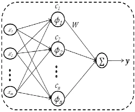
RBFNNs are found quite capable in terms of approximating functions and recognizing patterns [22]. In RBFNN an activation of a hidden neuron is determined based on the distance between an input and a sample vector. The figure of RBFNN is given below.
set of kernel units in the hidden layer from the input space to the hidden space. During the model training, the centres of prototype vectors are determined. Selection of appropriate quantity of basis functions which controls the approximation and the generalization ability of the network is an important issue in RBFNN. The different radial basis functions used in the RBFN are Gaussian, generalized multi-quadratic, generalized inverse multi-quadratic, thin plate spline, cubic, linear, and so on. We used the Gaussian functions as basis function as presented in Eq. 6.
−
−
=
2 22
exp
)
(
i i ix
x
(6)Where,
...
is the Euclidean norm andx
is the input vector.i i
,
and
i(
x
)
are the centre, spread, and output of theth
i
hidden node respectively. The output is calculated as in Eq. 7.
=−
=
=
N k k kk
x
c
w
x
f
y
1)
(
)
(
(7)Where
y
andx
represents the network output and inputvector respectively.
W
=
W
1,
W
2,
,
W
N
Tis the weight vector, the number of hidden neurons is N, and
k(.)
is the basis function. The bandwidth of the basis function is k. The vectorc
k=
(
c
k1,
c
k2,
,
c
km)
Tis the centre vector forth
k
node, and the input vector size is m.2.4. FLANN
In FLANN the higher-order effects at nodes are introduced through nonlinear functional transforms via links. The learning of a FLANN may be considered as approximating or interpolating a continuous, multivariate function
)
(X
f
by an approximating functionf
W(
X
)
. In FLANN aset of basis functions
and a fixed number of weight parameters W are used to representf
W(
X
)
. With a specific choice of a set of basis functions, the problem is to find the weight parameters W that provides the best possible approximation off
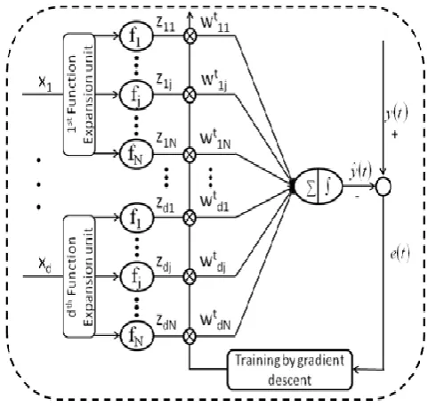
on the set of input-output examples. So, the most important thing is that how to choose the basis functions to obtain better approximation. FLANN based forecasting model is shown in Figure 3. As shown in figure, the input signals are fed to the functional expansion unit first. This unit uses few trigonometric functions for spreading out of each attribute of original input. The input vector consists here the historical daily closing prices of stock market. The inputs are normalized before feeding to the functional expansion unit. Let a d dimensional training sample isX
=
{
X
1,
X
2,
,
X
d}
. Each data point in the training sample is allowed to pass through the functionalunit consisting N number of trigonometric functions. The total number of expanded unit becomes
d
*
N
. Now these expanded signals are presented as input to the neurons at input layer. Therefore the total number of neurons at input layer isd
*
N
. In the Figure the levelsZ
11,
,
Z
dNare the expanded values for the input signals. The corresponding synaptic weight vector int
thiteration isW
=
{
W
11t,
W
1tN,
,
W
dNt}
. At the output neuron, (single neuron present in the output layer) the weighted sum of expanded signals and associated synaptic weight value is calculated. The output of this layer is passed through an activation function (sigmoid function) to produce the model responsey
ˆ
(
t
)
. The actual outputy
(t
)
is supplied to the output neuron and the error function is calculated. Now this error function is back propagated to update the weight and biases by gradient descent rule.Figure 3. FLANN based forecasting
Let us consider a set of basis function
i
L
A
iI=
(
)
with the following properties:(i)
I=1 (ii) the subset
j=
i
ij=1is a linearlyindependent set, i.e., if
=
=
j i i iw
10
)
(
, thenw
i=
0
for alli =1,2,…j, and
(iii)
= 2 / 1 1 2sup
j i A ij . Let
N i N
=
=1
be a setof basis functions to be considered for FLANN. Thus, the FLANN consists of N basis functions
N N
,
,
,
}
{
1 2
with the following input-output
=
=
=
N i i ji jj
s
w
X
s
y
1))
(
(
);
(
ˆ
(8)Where,
X
A
R
n, i.e.,X
=
[
x
1,
x
2,
,
x
n]
Tis theinput pattern vector,
y
ˆ
R
m, i.e.y
ˆ
=
[
y
1,
y
2,
,
y
m]
Tisthe output vector and
w
j=
[
w
j1,
w
j2,
,
w
jN]
is theweight vector associated with the
j
thoutput of the FLANN. The non-linear function
(.)
=
tanh(.)
is used to transfer the weighted sum into desired output format of an input pattern. Considering the m-dimension output vector, equation (5) can be written in matrix notation as follows.
=
W
S
(9),
Where, W is
m*
N
weight matrix of the FLANN given byW
=
[
w
1,
w
2,
,
w
m]
T,T
N
X
X
X
),
(
),
,
(
)]
(
[
1
2
=
is the basis functionvector, and
S
=
[
S
1,
S
2,
S
N]
Tis a matrix of linear outputs of the FLANN. The m-dimensional output vectory
ˆ
may be given by)
(
)
(
ˆ
S
f
X
y
=
=
w (10)The training of the network is done in the following way: Let ‘k’ patterns be applied to the network in a sequence
repeatedly. Let the training sequence be denoted by
)
,
(
X
ky
k and the weight of the network beW
(k
)
, where the ‘k’ is also the iteration. Referring to Equation (1) theth
j
output of the FLANN at iteration k is given by(
)
m
j
A
X
X
k
w
X
k
w
k
y
j T kN i k i ji
,
2
,
1
,
))
(
)
(
(
)
)
(
)
(
(
)
(
ˆ
1=
=
=
=
, (11)
Where,
(
X
k)
=
[
1(
X
1),
2(
X
2),
,
N(
X
k)]
T . Let the corresponding error be denoted by:)
(
ˆ
)
(
)
(
k
y
k
y
k
e
j=
j−
(12)In other words, the weighted sum of the functionally expanded features is fed to the single neuron of the output layer of the FLANN. The weighted sum of outputs obtained from the functional expansion units are then passed on to a sigmoid activation function at output unit. The estimated output is then compared with the target to obtain the error signal which is utilized to train the FLANN using the principle of gradient descent technique. Details about FLANN can be found in [12].
2.5 SVM
SVMs are supervised learning methods have been used widely for various data mining problems. It constructs a set
of hyper planes in a high dimensional space which can be used for classification or regression task. The hyper planes create a decision boundary so that most of the data points belong to one category fall on one side and data points belong to other class fall on the other side. The optimal hyper plane is one which maximizes the distance between the plane and any point termed as margin. Maximum the margin better is the splitting of data points. The selection of hyper plane depends upon the crucial elements closest to the boundary called as support vectors, hence the hyper plane is known as support vector classifier. SVM [23] can perform both linear & non-linear classification using different kernel functions which implicitly map their inputs into high-dimensional feature spaces. The original samples may be stated in a finite dimensional space which is not often linearly separable. Hence the original finite-dimensional space needs to be mapped into a much higher-dimensional space, making the separation easier. This is done by defining them in terms of a kernel function K x y( , ) selected to suit the problem. The commonly used kernel functions are linear, polynomial, RBF etc. We used the SVM implementation in MATLAB with the radial kernel.
3. Proposed method
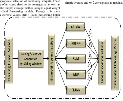
Selection of appropriate forecaster for modelling stock market trend is a critical and risky task. The ensemble framework suggested here attempts to overcome the risk of model selection as well as enhancing the overall prediction accuracy of the method. The framework combines five individual models such as ARIMA, RBFNN, SVM, MLP, and FLANN as shown in Figure 4. The process can be explained as follows. Let
X
i=
[
x
1,
x
2,
,
x
n]
Tbe the current training set generated from the original financial time series by sliding a window of fixed size through one step. The training set is then normalized using sigmoid data normalization method as ANN based models are performing better on normalized data. Now the normalized data is fed to individual forecasting models separately. Each forecaster transforms the input signalX
ito correspondingforecast
y
ˆ
i(
i
=
1
,
2
,
,
5
)
. A combination of the forecasts can be expressed as:)
,
ˆ
,
,
ˆ
,
ˆ
(
)
),
(
),
(
),
(
),
(
),
(
(
ˆ
5 21
y
y
W
y
f
W
X
FLANN
X
MLP
X
SVM
X
RBFNN
X
ARIMA
f
Y
i i i i i
=
=
(13)Where,
f
(.)
is a linear combination function and Tw
w
w
=
=
=
Ni
i k i
k
w
y
k
N
y
1
,
,
2
,
1
,
ˆ
*
ˆ
(14)Three statistical methods such as simple average, trimmed mean, and the median, as well as an error based method are used for appropriate selection of combining weights. These weights are often constrained to be nonnegative as well as unbiased. The simple average method assigns equal weight to all individual forecasting models. Though it is more sensitive to extreme values, still it found performing better
[24, 25]. The alternative statistical methods are trimmed mean and the median. Trimmed mean method averages the forecasts excluding
%
worst performing of the models. A 10-40% trimming is recommended [24, 25] and calculated as
=
100
*
(
2
/
n
)
. A
value zero corresponds to simple average andn
/
2
corresponds to median.Figure 4. Linear combination of forecasters
The trimmed mean is calculated as:
−+ =
=
−
=
ni i k
k
k
N
n
y
n
t
1
,
,
2
,
1
;
2
0
,
ˆ
2
1
)
(
(15)The combining weight to individual forecast in error based method is considered as the inversely proportional of the error generated by the corresponding model [23] and can be calculated as:
= −
=
ni i i i
err
err
w
1 1
(16)
Where,
err
iis the error generated byi
thforecasting model. This method assigns less weight to a model with more error and vice versa.It was observed from the literature that best accuracies are often obtained if forecasts are made through independent models and the combination method consist four to five
such models [5]. As per this guideline, we considered five models here to construct the ensemble framework. The overall process of ensemble framework can be explained by the high level algorithm as follows:
Algorithm 1: Ensemble framework
Input: The TrainData, TestData, and
n component
forecasting modelsM
i,
(
i
=
1
,
2
,
,
n
)
.
Output: The combined forecast through Eq.(10)
1. Normalization of TrainData and TestData
2. Fit the model
M
i to TrainData and update knowledge through learning3. Supply TestData to
M
i, and estimate the forecasts5. Obtain the final combined forecast as
1
ˆ
*
ˆ
n
i
k i k
i
y
w
y
=
=
4. Experimental results and
discussions
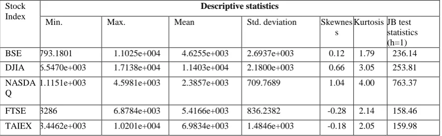
For experimental purpose daily closing indices from five fast growing stock markets such as DJIA, BSE, TAIEX, NASDAQ and FTSE are considered. The indices are collected from the source https://in.finance.yahoo.com/ for each financial day starting from 1st January 2003 to 12th September 2016. The descriptive statistics of these indices such as standard deviation, mean, minimum, maximum, skewness, kurtosis, and Jarque-Bera (JB) statistics are calculated and summarized in Table 1. it can be observed that DJIA, NASDAQ, and BSE data sets have shown positive skewness values and spread out more toward right further suggesting investment opportunities in these markets.
Similarly, real data from five exchange rates have been collected from the website www.forecasts.org. The data set consists of exchange rates of European Euro, British Pound, Indian Rupees, Japanese Yen, and Australian Dollar. The data show the average of daily figures on the 1st day of each month and collected for the period of 1999 to 2016. The number of data in each set is 214. The descriptive statistics
of the exchange rate series are summarized in Table 2. It can be observed that except Yen to Dollar and Pound to Dollar dataset all other datasets show positive skewness value. This means, these datasets are spread out more toward right and suggest investment opportunities. The kurtosis analysis implies that exchange rate of all datasets are less outlier prone than the normal distribution. Again from the Jarque-Bera test statistics, it can be observed that all the stock price datasets are non-normal distributed.
The patterns for training and testing the models are generated by using a sliding window technique. A window of fixed size is move over the financial time series by one step each time. In each move a new pattern has been formed which can be used as an input vector. The size of window can be decided experimentally. The original input data are then normalized using sigmoid normalization [26, 27] which is represented as in Eq. 17.
− − −
+
=
min max min
1
1
x x x x norm
i
e
x
(17)Here,
x
normandx
i are normalized and current day closingprice respectively,
x
max andx
minare the maximum and minimum prices of the current pattern respectively. The MAPE (Mean Absolute Percentage Errors) and ARVTable 1. Descriptive statistics from five stocks indices
Stock Index
Descriptive statistics
Min. Max. Mean Std. deviation Skewnes s
Kurtosis JB test statistics (h=1) BSE 793.1801 1.1025e+004 4.6255e+003 2.6937e+003 0.12 1.79 236.14 DJIA 6.5470e+003 1.7138e+004 1.1403e+004 2.1800e+003 0.66 3.05 253.81 NASDA
Q
1.1151e+003 4.5981e+003 2.3857e+003 709.7689 1.04 4.00 763.37
FTSE 3286 6.8784e+003 5.4166e+003 836.2382 -0.28 2.14 158.46 TAIEX 3.4462e+003 1.0201e+004 6.9834e+003 1.4846e+003 -0.18 2.05 159.98
Table 2 Descriptive statistics of exchange rates series from five stocks
Exchange rate series
Descriptive statistics
Minimum Maximum Mean Standard deviation
Yen/Dollar 76.6430 133.6430 106.2796 14.0317 0.5481 2.3795 14.1480(h=1) Australian
Dollar/Dollar 0.9276 1.9920 1.3393 0.2888 0.6141 2.4885 15.7831(h=1) Pound/Dollar 0.4831 0.7886 0.6161 0.0619 0.2110 2.6432 2.7234(h=0)
(Average Relative Variance) are used as the performance metrics whose formulas are as follows:
=
−
=
Ni i
i i
x
x
x
N
MAPE
1
%
100
ˆ
1
(18)
= =
−
−
=
Ni i N
i
i i
X
x
x
x
ARV
1
2 1
2
)
ˆ
(
)
ˆ
(
(19)
In these measures,
x
i andx
ˆ
iare the actual and estimatedclosing prices,
X
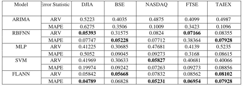
is the mean of data set. N is the total number of test data.As mentioned earlier, the experimental work is carried out with five forecasting models on five stock datasets. The performance of each model is calculated in terms of two metrics. For each financial time series the models are fed with same training and testing data. The MAPE and ARV obtained from individual models from five stock data sets are summarized in Table 3. The best ARV and MAPE values across a column (particular dataset) are in bold face letter. It can be observed that the performance of FLANN is better than other models followed by RBFNN. However there is no single method outperforming others over all data sets. Considering DJIA, the best ARV value, i.e. 0.05393 is obtained by RBFNN and the best MAPE value is obtained
by FLANN, i.e. 0.04789. For BSE dataset, the lowest ARV (0.05668) is generated by FLANN, where as the lowest MAPE (0.05228) is generated by RBFNN. For NASDAQ the lowest ARV (0.05827) is obtained by SVM and the lowest MAPE is generated by FLANN (0.05231). From FTSE, the lowest ARV is generated by RBFNN and the lowest MAPE is generated by FLANN again. Similarly, from TAIEX, the lowest ARV (0.08102) is obtained from FLANN and the lowest MAPE (0.07928) is obtained from FLANN and RBFNN both.
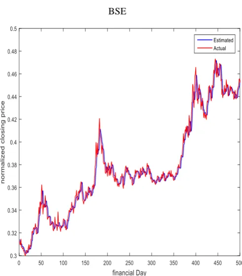
Similarly the performances of combination methods from all datasets are summarized in Table 4. The best metric values are highlighted with bold face letter. It can be observed that the ARV and MAPE values from all combination methods are found better than the best performing individual model which justifies improvement in prediction accuracies and overcome the risk of model selection. Even a small improvement in forecasting accuracy can create a reasonable profit, particularly the case of financial time series forecasting. Though the performance of error base combination method found better in case of three data sets, still there is lacking of a single method performing best across the data sets. Therefore utmost care should be taken while selecting a combination method over individual. The estimated and actual closing prices for all financial time series by combined methods are plotted by the Figures 5 – 9 respectively (first five hundred financial days only for better visibility).
Table 3. Performance of individual models on five data sets
Model Error Statistic DJIA BSE NASDAQ FTSE TAIEX
ARIMA ARV 0.5223 0.4035 0.4875 0.4099 0.4987
MAPE 0.6275 0.3506 0.1009 0.3423 0.1096
RBFNN ARV 0.05393 0.31575 0.0824 0.07166 0.08355
MAPE 0.07747 0.05228 0.07712 0.38364 0.07928
MLP ARV 0.41225 0.30685 0.47681 0.4139 0.5235
MAPE 0.5052 0.09045 0.09273 0.3168 0.08615
SVM ARV 0.41969 0.30633 0.05827 0.40681 0.40066
MAPE 0.19974 0.09242 0.07263 0.09273 0.08856
FLANN ARV 0.05842 0.05668 0.07832 0.08562 0.08102
MAPE 0.04789 0.06828 0.05231 0.06954 0.07928
Table 4. Performance of combined methods on five datasets
Combination Method
Error Statistic DJIA BSE NASDAQ FTSE TAIEX
Simple Avg. ARV 0.05349 0.05624 0.05703 0.07156 0.07902
Trimmed Mean ARV 0.03964 0.01856 0.0527 0.06023 0.08087
MAPE 0.03942 0.03987 0.03907 0.06595 0.07721
Median ARV 0.05085 0.05393 0.05809 0.05945 0.07909
MAPE 0.04727 0.03943 0.03957 0.06794 0.07886
Error Base ARV 0.02534 0.02562 0.05805 0.05037 0.07452
MAPE 0.03178 0.03751 0.03952 0.04433 0.06806
Figure 5. Actual v/s estimated closing prices by combined method (trimmed mean) from NASDAQ
Figure 7. Actual v/s estimated closing prices by combined method (error base) from
BSE
Figure 8. Actual v/s estimated closing prices by combined method (error base) from
FTSE
Figure 9. Actual v/s estimated closing prices by combined method (error base) from
TAIEX
Next we present and analyses the results obtained from exchange rate forecasting and the results obtained are presented by Table 5. The ARV and MAPE values from one-step-ahead forecasting are presented in Table 5 for all models. In this case also the FLANN, RBFNN, and SVM model found to be good in forecasting. For Rupees/Dollar time series, it is found that the lowest MAPE (0.04047) is obtained by RBFNN and lowest ARV (0.04490) is obtained by SVM model. The best MAPE and ARV values for Euro/Dollar are found by SVM and FLANN respectively. For Yen/Dollar the lowest MAPE and ARV values are obtained by RBFNN and FLANN respectively. For Australian Dollar/Dollar and Pound/Dollar series, the best ARV and MAPE values are generated by RBFNN and FLANN model respectively.
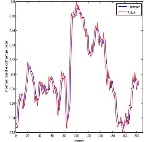
The performances of combination methods from all exchange rate series are summarized in Table 6. The best metric values are highlighted with bold face letter. As similar to closing prices forecasting, it can be observed that the ARV and MAPE values from all combination methods are found better than the best performing individual model which again justifies improvement in prediction accuracies over individual model. Here also the performance of error base combination method found better in case of two exchange rate series and still there is lacking of a single method performing best across the datasets. Therefore one should be extreme concern while selecting a combination method. The estimated and actual exchange rates for all time series by combined methods are plotted by the Figures 10 – 14 respectively. The plots show the closeness between the actual prices and estimated prices by the combination model.
Table 5 Performance of individual models on five exchange rate series
Model Error Statistic
Rupees/Dollar Euro/Dollar Yen/Dollar Australian Dollar/Dollar
Pound/Dollar
ARIMA ARV 0.55372 0.62355 0.24875 0.34095 0.42984
MAPE 0.32753 0.35166 0.64009 0.33825 0.10097
RBFNN ARV 0.07593 0.08357 0.08326 0.06560 0.08058
MAPE 0.04047 0.07025 0.02752 0.10083 0.07525
MLP ARV 0.09105 0.35680 0.47085 0.54037 0.52354
MAPE 0.05358 0.09541 0.20292 0.30016 0.09756
SVM ARV 0.04490 0.33629 0.07582 0.41685 0.24665
MAPE 0.07975 0.04245 0.08026 0.09675 0.08350
FLANN ARV 0.15045 0.05360 0.07532 0.08577 0.08405
MAPE 0.04288 0.06025 0.05501 0.06095 0.07225
Table 6. Performance of ensemble methods on five exchange rate series
Combination Method
Error Statistic
Rupees/Doll ar
Euro/Dollar Yen/Dollar Australian/Dol lar/Dollar
Pound/Dollar
Simple Avg. ARV 0.04345 0.04074 0.05370 0.05153 0.07935
MAPE 0.032292 0.04208 0.02051 0.05531 0.07005
Trimmed Mean ARV 0.03765 0.05150 0.07275 0.06025 0.08007
MAPE 0.031505 0.03962 0.02590 0.05595 0.06972
Median ARV 0.04082 0.04837 0.06800 0.05547 0.07999
MAPE 0.039628 0.03988 0.02495 0.05749 0.07018
Error Base ARV 0.02835 0.03956 0.05380 0.05235 0.07952
MAPE 0.032683 0.03827 0.02495 0.05433 0.06859
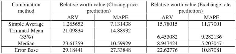
Table 7. Relative worth values of combination methods
Combination method
Relative worth value (Closing price prediction)
Relative worth value (Exchange rate prediction)
ARV MAPE ARV MAPE
Simple Average 1.265652 7.131438 15.78015 11.77001 Trimmed Mean
(35%)
21.09834 14.88932
6.453082 9.282136 Median 23.61359 10.59929 8.947424 5.203047 Error Base 29.18441 27.33848 22.62776 10.87081
Then, the relative worth
RW
jof thej
thcombination method is defined as follows:
=
=
−
=
Di
w i
ij w i
j
j
n
err
err
err
D
RW
1
,
,
2
,
1
,
100
*
1
(20) Where,
err
ijis the forecasting error generated by theth
j
method on thei
thdata,err
iws the error of bestindividual model for the same dataset, and D is the total number of datasets. The relative worth values (in terms of ARV and MAPE) are summarized in Table 7.
MAPE as compared to that of a best individual. Similarly the combined methods obtaining 6.45% to 22.62% ARV reduction and 5.20% to 11.77% MAPE reduction over the best performing individual models.
0 20 40 60 80 100 120 140 160 180 200 0.3
0.35 0.4 0.45 0.5
n
o
rm
a
li
ze
d
e
xcha
n
g
e
r
a
te
month
Estimated Actual
Figure 10. Actual v/s estimated exchange rate prices for Rupees/Dollar by combined method (trimmed mean)
0 20 40 60 80 100 120 140 160 180 200 0.3
0.35 0.4 0.45 0.5
n
o
rm
a
li
ze
d
e
xcha
n
g
e
r
a
te
month
Estimated Actual
Figure 11. Actual v/s estimated exchange rate prices for Euro/Dollar by combined method (error
based)
0 20 40 60 80 100 120 140 160 180 200 0.32
0.34 0.36 0.38 0.4 0.42 0.44 0.46 0.48 0.5
n
o
rm
a
li
ze
d
e
xcha
n
g
e
r
a
te
month
Estimated Actual
Figure 12. Actual v/s estimated exchange rate prices for Pound/Dollar by combined method (error based)
0 20 40 60 80 100 120 140 160 180 200 0.25
0.3 0.35 0.4 0.45 0.5
n
o
rm
a
li
ze
d
e
xcha
n
g
e
r
a
te
month
Estimated Actual
0 20 40 60 80 100 120 140 160 180 200 0.3
0.35 0.4 0.45 0.5
n
o
rm
a
li
ze
d
e
xcha
n
g
e
r
a
te
month
Estimated Actual
Figure 14. Actual v/s estimated exchange rate prices for Australian dollar/Dollar by combined method (simple
average)
5. Conclusions
Trend analysis in financial time series is a challenging and complex task as it is highly associated with uncertainties, nonlinearity, etc and talks to the current economical as well as political scenarios. Achieving enhanced forecasting accuracy is the key point while designing a model. Also, accurateness of an individual method/model is very much problem specific and exact identification of a best method is controversial. Combining outputs of different forecasting models to enhance overall accuracies and minimizing the risk of model selection has been suggested in literature. We suggested an ensemble framework of five individual ANN based models where the combination weights are assigned by simple statistical methods such as trimmed mean, simple average, median, and error based method. To maintain a trade-off between computational cost and predictive accuracy, we use simple methods for aggregating the individual models. Five state-of-the-art models such as ARIMA, RBFNN, MLP, SVM, and FLANN are used as the component model for the ensemble framework. The individual as well as combination models have been evaluated on predicting next day’s daily closing prices of five real stock markets and short term forecasting of five real global exchange rate series. From extensive simulation work it is clearly observed that the linear combiner methods producing better accuracies over all individual models. Particularly, the error base combination method found performing best among all which justified the approach of combining multiple forecasts as an alternative to individual. The relative worth of combined methods over individuals justified the significance of combine approach. However,
utmost care should be taken while selecting a combination method over individual. The work can be extended by choosing other neural base component models and exploring other aggregating methods for weight selection. Also, the combination model can be applied to other areas of time series forecasting.
References
[1] Terui, N. and Van Dijk, H.K., 2002. Combined forecasts from linear and nonlinear time series models. International Journal of Forecasting, 18(3), pp.421-438.
[2] De Gooijer, J.G. and Hyndman, R.J., 2006. 25 years of time series forecasting. International journal of forecasting, 22(3), pp.443-473.
[3] Andrawis, R.R., Atiya, A.F. and El-Shishiny, H., 2011. Forecast combinations of computational intelligence and linear models for the NN5 time series forecasting competition. International Journal of Forecasting, 27(3), pp.672-688.
[4] Adhikari, R. and Agrawal, R.K., 2014. Performance evaluation of weights selection schemes for linear combination of multiple forecasts. Artificial Intelligence Review, 42(4), pp.529-548.
[5] Armstrong, J.S. ed., 2001. Principles of forecasting: a handbook for researchers and practitioners (Vol. 30). Springer Science & Business Media.
[6] Kuncheva, L.I., 2004. Combining pattern classifiers: methods and algorithms. John Wiley & Sons.
[7] Tan, P.N., 2018. Introduction to data mining. Pearson Education India.
[8] Lemke, C. and Gabrys, B., 2010. Meta-learning for time series forecasting and forecast combination. Neurocomputing, 73(10-12), pp.2006-2016.
[10] Yu, L.Q. and Rong, F.S., 2010, May. Stock market forecasting research based on Neural Network and Pattern Matching. In 2010 International Conference on
E-Business and E-Government pp. 1940-1943. IEEE.
[11] Tahersima, H., Tahersima, M., Fesharaki, M. and Hamedi, N., 2011, June. Forecasting stock exchange movements using neural networks: A case study.
In 2011 International Conference on Future Computer
Sciences and Application pp. 123-126. IEEE.
[12] Pao, Y.H. and Takefuji, Y., 1992. Functional-link net computing: theory, system architecture, and functionalities. Computer, 25(5), pp.76-79.
[13] Majhi, R., Panda, G. and Sahoo, G., 2009. Development and performance evaluation of FLANN based model for forecasting of stock markets. Expert systems with applications, 36(3), pp.6800-6808. [14] Nayak, S.C., Misra, B.B. and Behera, H.S., 2018.
ACFLN: artificial chemical functional link network for prediction of stock market index. Evolving Systems, pp.1-26.
[15] Nayak, S.C., Misra, B.B. and Behera, H.S., 2015. Comparison of Performance of Different Functions in Functional Link Artificial Neural Network: A Case Study on Stock Index Forecasting. Computational Intelligence in Data Mining-Volume 1, pp. 479-487. [16] Nayak, S.C., Misra, B.B. and Behera, H.S., 2013,
September. Hybridzing chemical reaction optimization and artificial neural network for stock future index forecasting. In 2013 1st International Conference on Emerging Trends and Applications in Computer Science (pp. 130-134). IEEE.
[17] Nayak, S.C., Misra, B.B. and Behera, H.S., 2016. An adaptive second order neural network with genetic-algorithm-based training (ASONN-GA) to forecast the closing prices of the stock market. International Journal of Applied Metaheuristic Computing (IJAMC), 7(2), pp.39-57.
[18] Subramani, S., Michalska, S., Wang, H., Du, J., Zhang, Y. and Shakeel, H., 2019. Deep Learning for
Multi-Class Identification From Domestic Violence Online Posts. IEEE Access, 7, pp.46210-46224.
[19] Liu, F., Zhou, X., Wang, Z., Cao, J., Wang, H. and Zhang, Y., 2019. Unobtrusive Mattress-Based Identification of Hypertension by Integrating Classification and Association Rule Mining. Sensors, 19(7), p.1489.
[20] Peng, M., Zhu, J., Wang, H., Li, X., Zhang, Y., Zhang, X. and Tian, G., 2018. Mining event-oriented topics in microblog stream with unsupervised multi-view hierarchical embedding. ACM Transactions on Knowledge Discovery from Data (TKDD), 12(3), p.38 [21] Box, G.E., Jenkins, G.M., Reinsel, G.C. and Ljung,
G.M., 2015. Time series analysis: forecasting and control. John Wiley & Sons.
[22] Dash, C.S.K., Dash, A.P., Dehuri, S., Cho, S.B. and Wang, G.N., 2013. DE+ RBFNs based classification: A special attention to removal of inconsistency and irrelevant features. Engineering Applications of Artificial Intelligence, 26(10), pp.2315-2326.
[23] Halls-Moore, M., 2014. Support vector machines: A guide for beginners.
[24] Lemke, C. and Gabrys, B., 2010. Meta-learning for time series forecasting and forecast combination. Neurocomputing, 73(10-12), pp.2006-2016.
[25] Jose, V.R.R. and Winkler, R.L., 2008. Simple robust averages of forecasts: Some empirical results. International Journal of Forecasting, 24(1), pp.163-169.
[26] Nayak, S.C., Misra, B.B. and Behera, H.S., 2014. Impact of data normalization on stock index forecasting. Int. J. Comp. Inf. Syst. Ind. Manag. Appl, 6, pp.357-369.
[27] Nayak, S.C., Misra, B.B. and Behera, H.S., 2012, October. Evaluation of normalization methods on neuro-genetic models for stock index forecasting.
In 2012 World Congress on Information and