A Study of Distance Metrics in Histogram Based Image Retrieval
Abhijeet Kumar Sinha, K.K. Shukla
Department of Computer Engg. , IIT(BHU), Varanasi
[email protected]
Department of Computer Engg. , IIT(BHU), Varanasi[email protected]
ABSTRACT
There has been a profound expansion of digital data both in terms of quality and heterogeneity. Trivial searching techniques of images by using metadata, keywords or tags are not sufficient. Efficient Content-based Image Retrieval (CBIR) is certainly the only solution to this problem. Difference between colors of two images can be an important metric to measure their similarity or dissimilarity. Content-based Image Retrieval is all about generating signatures of images in database and comparing the signature of the query image with these stored signatures. Color histogram can be used as signature of an image and used to compare two images based on certain distance metric.
In this study, COREL Database is used for an exhaustive study of various distance metrics on different color spaces. Euclidean distance, Manhattan distance, Histogram Intersection and Vector Cosine Angle distances are used to compare histograms in both RGB and HSV color spaces. So, a total of 8 distance metrics for comparison of images for the sake of CBIR are discussed in this work.
General Terms
Content-based Image Retrieval, Image Processing, Histograms
Indexing terms
Content-based Image Retrieval (CBIR), Euclidean distance, Manhattan distance, Vector Cosine Angle distance, Histogram Intersection Distance, COREL database
Academic Discipline And Sub-Disciplines
Computer Science & EngineeringSUBJECT CLASSIFICATION
Image RetrievalTYPE (METHOD/APPROACH)
Quasi-Experimental1. INTRODUCTION
With the growing need of digital data and declining cost of storage, we have moved past the trivial text-based search of images and advanced towards Content-based Image Retrieval. The focus is now upon the efficient methods and features to be used to get semantically best results. Computers are better at measuring properties and storing it in their memory; however, humans are much better than computers at attaching semantic description to an image [1].This is still an open question as to which method is the best as each has its own pros and cons but some major works has been done in this direction in [1][2][3]. The common ground of all the CBIR techniques is to extract the signature of the query image on the basis of its pixel values and compare it with already stored signatures of all the images in the database based on some rule. This comparison rule can be some distance metric, as discussed in this paper, or some other rules based on local characteristics. According to [3], besides providing significant compression of image representation, signatures also provide an improved correlation between image representation and semantics. The meaning of the image is inferred based upon the signature derived from pixel values. Most of the CBIR techniques use one of the 3 approaches to extract signatures: histogram, color layout and region-based search [3]. Color histogram is an important feature of an image which gives a global representation of an image; it gives a holistic view of an image. However, there are references available in the literature which focuses upon a certain portion of the image and semantically distinguish it on the basis of that [4]. Two histograms are compared on the basis of certain distance metric. Several distance metrics are available in the literature: Euclidean distance, Manhattan distance, Vector Cosine Angle distance, Histogram Intersection distance, CIEdeltaE, CIEdeltaE2000, Earth Mover’s distance [5] and many more. The results vary greatly on the distance metrics, the color space and also on the image database used. In this paper, an exhaustive study of effects of various distance metrics in different color spaces has been done. Euclidean distance, Manhattan distance, Histogram Intersection distance and Vector Cosine Angle distance are used to measure similarity between two images in each of the two color spaces, viz RGB and HSV. In all, there are 8 approaches used whose performance is measured by precision and recall [6]. COREL database is used for the study. In COREL database there are 1000 images distributed in 10 categories, each of them having 100 images.
used in this work has been discussed. In section 4, the experiments and results of the work have been detailed. The last section draws conclusion from the work so done and discusses some future work.
2. COLOR SPACE
Color space is a digital palette with colors being much precisely organized and quantified. It relates colors to a tuples of numbers, typically to three or four values or color components. Different color spaces are available in literature. In this paper, RGB and HSV color spaces have been used for study.
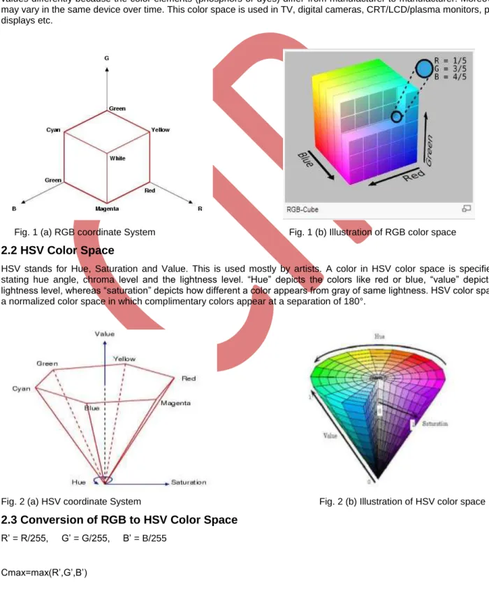
2.1 RGB Color Space
RGB color model is an additive color model in which Red(R), Green(G) and Blue(B) are added together in order to produce an array of colors. RGB is a device dependent color space. Different devices detect or produce a given RGB values differently because the color elements (phosphors or dyes) differ from manufacturer to manufacturer. Moreover, it may vary in the same device over time. This color space is used in TV, digital cameras, CRT/LCD/plasma monitors, phone displays etc.
Fig. 1 (a) RGB coordinate System Fig. 1 (b) Illustration of RGB color space
2.2 HSV Color Space
HSV stands for Hue, Saturation and Value. This is used mostly by artists. A color in HSV color space is specified by stating hue angle, chroma level and the lightness level. “Hue” depicts the colors like red or blue, “value” depicts the lightness level, whereas “saturation” depicts how different a color appears from gray of same lightness. HSV color space is a normalized color space in which complimentary colors appear at a separation of 180°.
Fig. 2 (a) HSV coordinate System Fig. 2 (b) Illustration of HSV color space
2.3 Conversion of RGB to HSV Color Space
Cmin=min(R’,G’,B’) Δ = Cmax-Cmin Hue calculation: H= (i) Saturation calculation: S= (ii) Value calculation: V=Cmax (iii)
2.4 Conversion of HSV to RGB Color Space
0 ≤ H ≤ 360° , 0 ≤ S ≤ 1 , 0 ≤ V ≤ 1 C= V S X= C (1-|(H/60°) mod 2 – 1|) m=V-C (R’, G’, B’) = (iv) (R, G, B) = (R’+m, G’+m, B’+m) (v)
3. DISTANCE METRICS
We store the color histograms of all the images in the database. Once given the query image, its signature, i.e color histogram, is calculated and thereafter its distance from all those present in the database. Accordingly, the results are sorted and nearest neighbors are displayed. In this work, 4 distance metrics have been used as a similarity rule.
3.1 Euclidean Distance
In Cartesian coordinates, if X = (x1, x2... xn) and Y = (y1, y2... yn) are two points in Euclidean n-space, then the Euclidean distance between X and Y is given by:
E(X, Y) = = (vi)
3.2 Manhattan Distance
If X = (x1, x2... xn) and Y = (y1, y2... yn) are two points, then the Manhattan distance between X and Y is given by:
M(X, Y) = |x1 - y1| + |x2 - y2| + .... + |xn – yn| = (vii)
3.3 Histogram Intersection Distance
It was proposed in [11]. Let IR, IG and IB be the normalized color histograms of an image in the database and let QR, QG
and QB be the normalized color histogram of query image. The similarity between the query image and the stored image in
the database, SCHI(I,Q) is given by:
(viii)
SCHI(I,Q) lies the interval [0,1]. If the histograms I and Q are identical then SCHI(I,Q)=1. Moreover, if either of the twoimages is completely contained in the other, then SCHI(I,Q)=1 [11].
3.4 Vector Cosine Angle Distance
The cosine of angle between two vectors determines whether two vectors are pointing in roughly the same direction. This distance is frequently used in data mining to measure the cohesion within clusters. If X = (x1, x2... xn) and Y = (y1, y2... yn) are two points, then cosϴ is the cosine of vector angle between X and Y in n-dimension.
(ix)
4. EXPERIMENTS & RESULTS
In this paper, we have used COREL database for the experiment purpose. COREL database consists of 1000 images divided in 10 categories with 100 images in each category. The categories of the images are people, beach, monuments, buses, dinosaurs, elephants, flowers, horses, mountains and cuisines. First of all, signatures of all the images are stored in a database and then an image is queried with its signature as input. In this work, we have color histogram of an image as the signature. The rule for similarity measure is distance metrics. 4 different distance metrics, viz, euclidean distance, manhattan distance, histogram intersection distance and vector cosine angle distance, are used in two color spaces, RGB and HSV. Thus, in all we have 8 different rules for similarity measures for content based retrieval. The performance criteria are precision and recall.
4.1 Calculating Precision
As discussed in [6], precision is defined as the ratio of number of relevant images retrieved to number of images retrieved.
Precision =
Recall =
Fig. 3 Venn diagram illustrating Precision and Recall
Let A be the set of relevant images and B be the set of retrieved images. In the above image, a stands for unretrieved relevant images, b stands for relevant retrieved images and c stands for retrieved irrelevant images [9].
Recall = P(B|A) = = (x)
Precision = P(A|B) = = (xi)
The better the precision at same recall value, the better the distance metric is. Here, because we use COREL database, the number of relevant images is fixed, 100.
We calculate precision of the distance metric by varying the number of retrieved images. Once, the distance of query image is calculated with all the images in the database, it is sorted. The order of sort depends on the type of distance metric. So, the denominator for calculating precision (No. of images retrieved) is varied by considering 10, 20 and 30 nearest neighbors (NN). Out of these nearest neighbors (NN), how many of them belong to the same category as the query image, that’s precision.
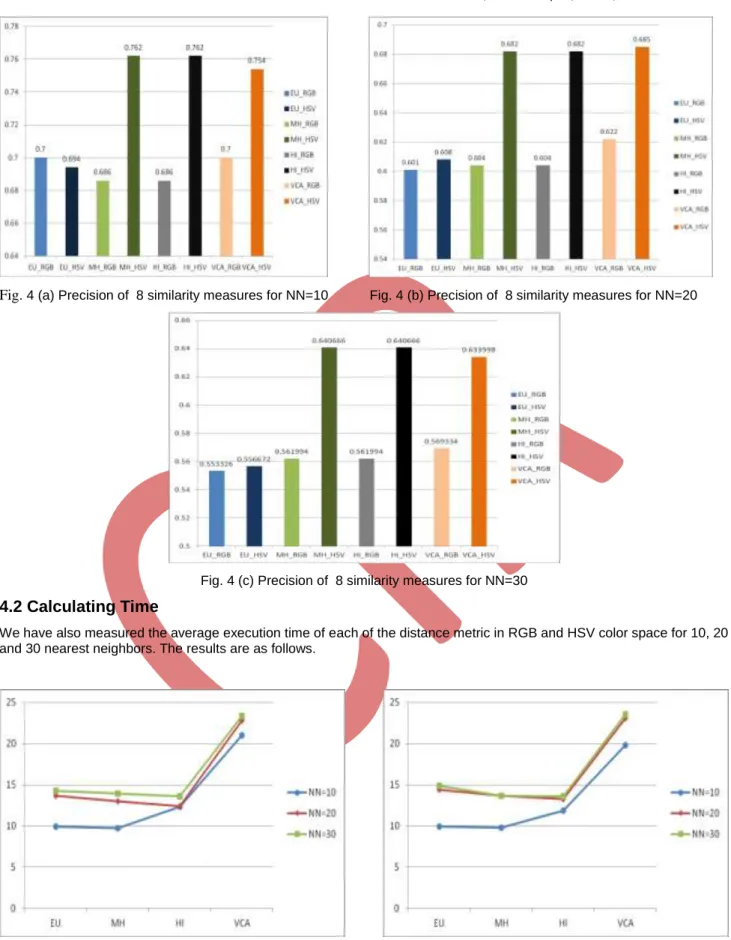
For, the purpose of experiment, we have considered 5 random images from each of the 10 category as the query image and calculated their precision based on all the 4 distance metrics in both the color spaces. Then we have taken the mean of the precision of all the 50 images for each of the 8 similarity rules (4 distance metrics each in 2 color spaces). The above process is repeated for 3 cases, when the no. of images retrieved is 10, 20 and 30. A bar graph is subsequently plotted to discuss the results.
Fig. 4 (a) Precision of 8 similarity measures for NN=10 Fig. 4 (b) Precision of 8 similarity measures for NN=20
Fig. 4 (c) Precision of 8 similarity measures for NN=30
4.2 Calculating Time
We have also measured the average execution time of each of the distance metric in RGB and HSV color space for 10, 20 and 30 nearest neighbors. The results are as follows.
Fig. 5 (a) Execution time for 4 distance metrics in RGB Fig. 5 (a) Execution time for 4 distance metrics in HSV color space color space
4.3 Calculating Recall vs Precision
Recall vs. Precision graphs were plotted for each of the separate category of images from COREL database. For each of the category 5 images were considered and their average was taken. For 10 recall values (0.1 to 1), precisions were calculated and subsequently plotted.
Fig. 6 (a) Recall vs. Precision (Dinosaurs) Fig. 6 (b) Recall vs. Precision (Horses)
Fig. 6 (c) Recall vs. Precision (Cuisines) Fig. 6 (d) Recall vs. Precision (Monuments)
Fig. 6 (e) Recall vs. Precision (Buses) QUERY IMAGE
Manhattan (RGB) Manhattan (HSV)
Histogram Intersection (RGB) Histogram Intersection (HSV)
Vector Cosine Angle (RGB) Vector Cosine Angle (HSV)
Fig. 7 Best two retrieved images for each of the distance metrics
4.4 Results
Given a query image, Fig. 7 displays two retrieval results for each of the 8 similarity rules. In this one, Histogram
Intersection distance seems to perform very well; but the two retrieved images are from different categories, although their color information seems to be same. Some more tests were also performed. But it was hard to find some general trend based on subjective tests.
From the bar graphs of precision, Fig. 4 (a) ~ (c), we conclude that Manhattan Distance and Histogram Intersection Distance comes out as winners among all the distance metrics. Moreover, the result is much better in HSV color space than RGB color space.
The time plots, Fig. 5 (a) ~ (b), show almost the same execution time in both the color spaces. The transformation factor from RGB to HSV color space is marginal. As expected, taking into account 30 nearest neighbors took a little bit more execution time than 20 nearest neighbors which in turn took some more time than 10 nearest neighbors. Both the color spaces gave uniform results in terms of execution time.
The more the precision at a certain recall, the better is the image retrieval. The recall vs. precision graphs, Fig. 6 (a) ~ (e), show that in most of the cases HSV color space performed better that RGB color spaces. In all the cases, except Horses category, Histogram Intersection distance performed much better that any of the other distance metric.
So, overall Histogram Intersection distance in HSV color space turns out to be the best distance metric for histogram, based image retrieval. It gives the best precision and takes the least time among all the similarity measures.
5. CONCLUSIONS
In this work, four distance metrics were compared in two color spaces. According to the precision graph and time graph, we conclude that Histogram Intersection distance is the best method among these four. It gives the most satisfying precision and takes the least computation time. Vector Cosine Angle distance (VCAD) is computationally burdensome because of a number of multiplications and divisions involved. It is intelligible from the time plot where execution time of VCAD just shoots up in both the color spaces. HSV color space results in better performance than RGB color space. Execution time difference between the two color spaces is marginal.
However, histogram approach is a method of global image representation. It discards the information about texture, shape and location. There can be semantic differences between the images retrieved even if their color information may be the same. For future work, rather than using histograms to extract signatures, we can also use color layout [1] [13] or region-based methods to extract signatures and then do performance analysis. Color-layout method retains the information regarding shape, texture and shape; however, it is sensitive to shifting, cropping, scaling and rotation. Region-based methods [16][17] attempts to overcome the drawbacks of color-layout by acting at object level. Moreover, some other distance metrics like Earth Mover’s distance [5] and weighted Euclidean distance [1] [7] can also be considered for performance analysis.
ACKNOWLEDGMENTS
Our sincere thanks to the expert faculty members and friends who helped us with this work.
REFERENCES
[1] M. Flickner, H. Sawhney, W. Niblack, J. Ashley, Q. Huang, B. Dom et al. "Query by Image and Video Content: The QBIC System," IEEE Computer, vol. 28, no. 9, 1995. A. Natsev, R. Rastogi, and K. Shim, "WALRUS: A Similarity Retrieval Algorithm for Image Databases," SIGMOD Record, vol. 28, no. 2, pp. 395-406,1999.
[2] A. Natsev, R. Rastogi, and K. Shim, "WALRUS: A Similarity Retrieval Algorithm for Image Databases," SIGMOD Record, vol. 28, no. 2, pp. 395-406,1999.
[3] J. Wang, J. Li, and G. Wiederhold. "SIMPLIcity: Semantics-sensitive Integrated Matching for Picture Libraries". IEEE Transactions on Pattern Analysis and Machine Intelligence, pages 947–963, 2001.
[4] R. Rahmani, S. Goldman, H. Zhang, J. Krettek, & J. Fritts. (2005). Localized content-based image retrieval. MIR, 227–236.
[5] Yossi Rubner, Leonidas Guibas, Carlo Tomasi ,"The Earth Mover's Distance, Multi-Dimensional Scaling, and Color-Based Image Retrieval", Int. J. Comput. Vision 40, 99–121.
[6] S. Aksoy and R. M. Haralick. “Content-based image database retrieval using variances of gray level spatial
dependencies”. In Proceedings of IAPR International Workshop on Multimedia Information Analysis and Retrieval, Hong Kong, August 1998.
[7] J. Hafner, H. S. Sawhney, W. Equitz, M. Flickner, and W. Niblack. “Efficient color histogram indexing for quadratic
form distance functions”. IEEE Transactions on Pattern Analysis and Machine Intelligence, 17(7):729{735, July 1995.
[8] A., Majumdar, A.K., Sural, S., 2003. “Performance comparison of distance metrics in content-based image retrieval
applications”. In: Proc. of Internat. Conf. on Information Technology, Bhubaneswar, India, pp. 159–164.
[9] Jeong, Sangoh. “Histogram-Based Color Image Retrieval”, Psych221/EE362 Project Report, Stanford University,
2001.
[10] Rishav Chakravarti, Xiannong Meng, A study of Color Histogram Based Image Retrieval , 2009 Sixth International Conference on Information Technology: New Generations
[11] A. Jain and A. Vailaya. “Image Retrieval using Color and Shape”, Pattern Recognition, 29(8), pp. 1233–1244, 1996. [12] A. Gupta and R. Jain, “Visual Information Retrieval”, Comm. ACM, vol. 40, no. 5, pp. 70-79, May 1997.
[13] J.Z. Wang, G. Wiederhold, O. Firschein, and X.W. Sha, "Content-Based Image Indexing and Searching Using Daubechies' Wavelets", Int'l J. Digital Libraries, vol. 1, no. 4, pp. 311-328, 1998.
[14] J. Shi and J. Malik, "Normalized Cuts and Image Segmentation", Proc. Computer Vision and Pattern Recognition, pp. 731-737, June 1997.
[15] A. Vailaya, A. Jain, and H.J. Zhang, "On Image Classification: City versus Landscape", Proc. IEEE Workshop Content-Based Access of Image and Video Libraries, pp. 3-8, June 1998
[16] C. Carson, M. Thomas, S. Belongie, J.M. Hellerstein, and J. Malik,"Blobworld: A System for Region-Based Image Indexing and Retrieval", Proc. Visual Information Systems, pp. 509-516, June 1999.
Processing, pp. 568-571, 1997.