A spatial dynamic approach to ecological modeling: Simulating fire spread.

A spatial dynamic approach to ecological

modeling: Simulating fire spread.

Authors Ball, George LeRoy.

Publisher The University of Arizona.

Rights Copyright © is held by the author. Digital access to this material is made possible by the University Libraries, University of Arizona. Further transmission, reproduction or presentation (such as public display or performance) of protected items is prohibited except with permission of the author.

Download date 19/01/2021 01:56:41

The most advanced technology has been used to photograph and reproduce this manuscript from the microfilm master. UMI films the text directly from the original or copy submitted. Thus, some thesis and dissertation copies are. in typewriter face, while others may be from any type of computer printer.

The quality of this reproduction is dependent upon the quality of the copy submitted. Broken or indistinct print, colored or poor quality illustrations and photographs, print bleed through, substandard margins, and improper alignment can adversely affect reproduction.

In the unlikely event that the author did not send UMI a complete manuscript and· there are missing pages, these will be noted. Also, if unauthorized copyright material had to be removed, a note will indicate the deletion.

Oversize materials (e.g., maps, drawings, charts) are reproduced by sectioning the original, beginning at the upper left-h:md corner and continuing from left to right in equal sections with small overlaps. Each original is also photographed in one exposure and is included in reduced form at the back of the book.

Photographs included in the original manuscript have been reproduced xerographically in this copy. Higher quality 6" x 9" black and white photographic prints are available for any photographs or illustrations appearing in this copy for an additional charge. Con~act UMI directly to order.

U·l'vI·I

UniverSity Microfilms International A B811 & Howell Information Company

300 North Z8eb Road. Ann Arbor. MI 48106·1346 USA 313 761·4700 800521·0600

A spatial dynamic approach to ecological modeling: Simulating fire spread

Ball, George LeRoy, Ph.D.

The University of Arizona, 1990

V·M·I

A SPATIAL DYNAMIC APPROACH TO ECOLOGICAL MODELING: SIMULATING FIRE SPREAD

by

George LeRoy Ball

A Dissertation Submitted to the Faculty of the SCHOOL OF RENEWABLE NATURAL RESOURCES In Partial Fulfillment of the Requirements

For the Degree of DOCTOR OF PHILOSOPHY In the Graduate College THE UNIVERSITY OF ARIZONA

GRADUATE COLLEGE

As members of the Fi.nal Examination Committee, we certify that we have read the dissertation prepared by __ ~G~e~o~~~g~e~:L~e~R~o~y~B~a~1~1 ____________________ __

entitled A SPATIAL DYNAMIC APPROACH TO ECOLOGICAL MODELING: SIMULATING FIRE SPREAD

and recorrmend that it be accepted as fulfilling the dissertation requirement for the Degree of Docto~ of Ph 11 osophy

---~--- \)

,?tJ/~ G~i-~

D. PhIllIp Gue~tln Date

'3ba£u>4.-

~'

'f!~

Wl1llamB. Heed Date

"Rtet1-,~ ~ ~Y'Cl''V'44.

3 / 29 / 90

Rlcha~d St~auss Date

Final approval and acceptance of this dissertation is contingent upon the candidate's submission of the final copy of the dissertation to the Graduate College.

I hereby certify that I have read this dissertation prepared under my direction and recommend that it be accepted as fulfilling the dissertation requirement.

3/29/90

STATEMENT BY AUTHOR

This dissertation has been submitted in partial fulfillment of requirements for an advanced degree at The University of Arizona and is deposited in the University Library to be made available to borrowers under rules of the library.

Brief quotations from this dissertation are allowable without special permissio:il, provided that accurate

acknowledgment of source is made. Requests for permission for extended quotation from or reproduction of this

manuscript in whole or in part may be granted by the head of the major department or the Dean of the Graduate College when in his or her judgment the proposed use of the 'material

is in the interests of scholarship. In all other instances, however, permission must be obtained from the author.

ACKNOWLEDGMENTS

I would to take this opportunity to thank some great friends: Bill Heed and Rich strauss for encouragement as a biologist; Mal Zwolinski for teaching me about fire; Randy Gimblett for introducing me to AI; and Phil Guertin who has shown me how to survive in academia. I want to thank my friends in the Advanced Resource Technology Program for their support, and the College of Agriculture for supplying the equipment. And most of all I want to thank my mother and sister for all their help, support and a place ' .. 0 live

TABLE OF CONTENTS Page LIST OF ILLUSTRATIONS 7 LIST OF TABLES .••...••••••...••.••...• 8 ABSTRACT • . . . • . . . • • • • • • . . . • • . . . • 9 INTRODUCTION • • . . . • • • • • • . . . • . . . 11 SECTION 1 1.1 The Form of Ecosystems • • . . . • . • • . . . • . • . . 15

1.2 An Examination of Current Models . . . • . . . 18

SECTION 2 2.1 Representing the Physical Environment . . . • . . . . 22

2.1.1 Data Capture . • • • • • . . . • . . . 23

2.1.2 Georeferenced Data . . . . • . . . • . . . 24

2.1.3 Cell Resolution • • . . . 25

2.2 Methods of Data Analysis . . . • . . • . . . 25

2.2.1 Mathematical Surfaces . . . . • . . . • . . . 26

2.2.2 Analytical Operators • . • • . . . 27

2.3 Models Using GIS Programs • . . • . . . • . . . 29

2.4 Criteria for Designing a Simulation Program .. 30

2.4.1 First criterion: Real Numbers . . . 30

2.4.2 Second criterion: Iterative Processing .. 32

2.4.3 Third Criterion: Flexibility in Data Retrieval • • • . . . • • . • • . . . 33

2.4.4 Fourth criterion: Neighborhood Analysis .33 SECTION 3 3.1 Vector and Raster Systems . . . . • . . . • . . 35

3.1~1 Vector suitability . • . . . 35

3.1.2 Raster suitability • . . . • • . . . 36

3.2 The PROMAP Basic Configuration . . . 38

3.2.1 File Structure • . • . . . • . . • . . . 39

3.2.2 Memory Structure • . • . . . 40

3.2.3 Operators • • . . • . • • . . . 40

3.2.4 Mathematical Procedures . . • • . . . 46

3.2.5 Programmable operation . . . 47

3.2.5.1 Example of the CELL operator •..••. 48

SECTION 4 4.1 Modeling Biophysical System Processes . . . 51

4.1.1 Representing the Environment . . . 51

TABLE OF CONTENTS CONTINUED

Page

4.2 Developing Transition Functions .•••.••...•...••.. 54

4.2.1 spatial Transition Functions •...•.••.... 54

4 • 2 • 2 Timing . . . 55

SECTION 5 5.1 Fire as a Spatial Dynamic Modeling Problem . . . . 56

5.1.1 Factors Which Define Fire . . . . • . . . • . . . • 56

5.1.1.1 Fuels ••••.•••.••••••...••...•... 57

5.1.1.2 Fuel Moisture •••••.••••..•••....•. 57

5.1.1.3 Slope and Wind ••.•.••..•...•••.... 58

5.1.2 Dynamic Aspects of Fire . . . • • . . . • . 58

5.2 The Rate of Spread Equation ••..••..••....••... 59

5.2.1 Basic Problems with the Fire Equations •• 61 5.3 FIREMAP ••••••••••••••••••••••••••...••...•. 62

5.3.1 Problems in FIREMAP • . . • • . . • . . • . . • . . . 63

5.4 Other Fire Spread Models ••••.•...•...••.... 64

SECTION 6.1 6 FIREMAP II • • . • • . • • . • . • . . . • . . . • . . . 69 6.2 6.3 SECTION 7.1 7.2 SECTION 8.1 8.2 8.3 8.4 6.1.1 Algorithm for Fire Spread • • • . . . 69

6.1.1.1 Flanking ROS Equation . . . • . . . • . . 72

6.1.2 The Fire Spread Operators • • . . . 73

Testing Zero State Predictions . . . • • . . • • . . . 76

Testing Non-uniform Conditions • . . . 80

7 Identified Errors • • • • . • • . . . 84

7.1.1 The Adjusted ROS ••••....•.••...•... 84

7.1.2 Wind Fields . • . . . • . . . 85

Simulation Benchmarks ••••••...•...•... 86

8 An Evaluation of PROMAP/FIREMAP . • . . . 87

Recommendations for Improvement of FIREMAP . . . . 89

8.2.1 Wind Fields . . • • . . . . • . • . • . . . 89

8.2.2 Rules for Extinguishing Fires . . . 90

8 . 2 . 3 F ire Breaks . • . . . • . . . • . . . 90 Future Implications • • . . • • • . . . • . . . 91 8.3.1 Fire Ecology ...•....•..•••....••.••.. 91 8.3.2 Animal Habitat • . • • . . . 92 8.3.3 Risk Management • . . . . • . . . • • . . . 93 Conclusion • . • • . . • • • . • • • . . . 94 LITERATURE CITED . . . • • . • . . . . • . . . 96

List of Figures

Figure Page

1. PROMAP Memory structure ••••.••...••••...•... 41

2. CELL Operator Script File • • . . • . . . • . • . . . . • . . . 49

3. Results of Script File in Figure 2 . . . • . . 50

4. The Cellular Neighborhood of Fire . . • . . . 70

5. Fire Spread Zero Wind Speed • • • • • • . . . 78

6. Fire Spread 2 mph Wind Speed · • • . • . . . • • 78

7. Fire Spread 4 mph Wind Speed • • . . • . . . • . . . • . 79

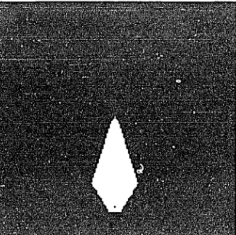
8. Fire Spread 8 mph Wind Speed · ••••.••... 79

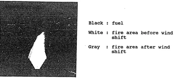
9. Fire Spread 4 mph with Wind Shift •.•••....•... 81

10. Fire Spread 8 mph with Barrier . • . . . 81

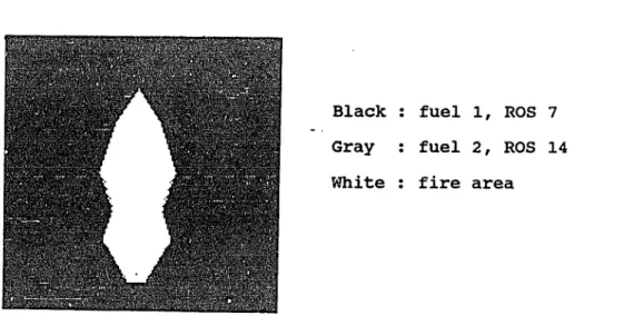
11- Fire Spread 4 mph with 2 Fuels • . . . . • . . . 82

List of Tables page

Table

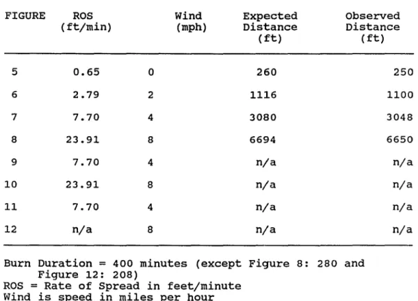
1. PROMAP Opera tors •••••••••.•••..•••..••...•...•. 4-2 2. Results of Fire simulations •••••••..•..•••...•.. 77

ABSTRACT

The objective of this dissertation is to develop a new research tool, PROMAP, which will allow the construction of models that satisfy the requirements of spatial distribution and hierarchical interactions within a dynamic framework.

An analysis of the form of ecosystems is followed by an examination of current attempts at ecosystem modeling using spatial relationships. An examination of the analytical procedures used in the spatial modeling process, results in a set of criteria that a suitable modeling system should incorporate. These criteria are: the use of real numbers; iterative processing; flexible data retrieval; and

neighborhood analytical procedures.

The basic configuration of PROMAP is discussed with an emphasis on the mathematical procedures and the capability for designing cellular automata within the system. The representation of biophysical systems into a set of spatial transition functions is described in relation to the

development of nested hierarchies called Q-morphisms. Having established the design of PROMAP, a suitablE! test is devised using the simulation of surface fire spread. A model called FIREMAP is developed and the results are compared to expected fire shapes under Zero state

zero slope and zero wind with additional factors held cons'tant. Other simulations of fire spread are made by relaxing the conditions to achieve wind driven fires and the response to potential impediments to fire spread. The

response of the simulation shows an accurate correspondence between the simulation and the expected fire shape.

As a final test of the model, all restrictions are removed and a simulation is made under actual conditions of complex terrain, and non-uniform fuels using data collected on the San Carlos Apache Indian Reservation in southeast Arizona.

Deficiencies of PROMAP and FIREMAP are discussed as well as future implications for the FIREMAP model as a management tool.

INTRODUCTION

Eldredge and Cracraft (1980) point to the perception of

different patterns in nature. Ecological order in the

biotic world gives the perception of hierarchical

structure, and distributional aspects show patterns in time

and space. To develop a realistic model of a natural

system, a model must describe the system hierarchically in time and space.

Models are generally constrained· by the inability to measure and use all the variables that would be necessary

to describe natural systems. To make the modeling process

more tractable assumptions are made about some variables,

such as "negligible influence" or "held constant". Which

variables are considered important and which are not is decided by the modeler and how well the model simulates the

real world. Spatial distribution imposes the additional

requirements of locational identity and neighborhood

interaction. Although the lack of spatial distribution

prevents the examination of hierarchical interaction in space, i t does not necessarily prevent examination through time.

The objective of this dissertation is to develop a new research tool, PROMAP, which will allow the construction of models that satisfy the requirements of spatial

framework (i.e., spatial dynamic models). PROMAP is a spatial dynamic simulation language which provides the necessary operators to access and manipulate spatially referenced information to simulate the interactions found in natural ecosystems. As a test of the functionality of PROMAP, it has been applied to the modeling of surface fire spread in a natural system.

The spread of surface fire in natural systems has been the subject of much scientific investigation and there exists a large body of literature describing observed pa"tterns as well as empirical data relating fire behavior, fuels and meteorology. The variability within this system, as in any natural system, precludes the ability to make absolute predictions. The application of empirically derived procedures to actual fire situations has shown the efficacy of equations for rate of spread and other

components of fire behavior. The test of this dynamic spatial modeling system would be the ability of the model to produce the expected shape of a fire under a set of specified conditions. The fire shapes generated by the model must be derived from known characteristics of fire behavior. The model has been given thp. name FIREMAP.

section 1 will discuss the form of ecosystems and examine some current models and their deficiencies in trying to describe natural systems. section 2, will

examine how biophysical environments can be d~scribed as database structures, and what analytical procedures can be applied. This section describes the primary design

criteria for PROMAP. section 3 examines two competing data structures and the PROMAP program. This section outlines the basic components of the PROMAP system, discusses some of it's more powerful operators, and gives examples of how the operators are applied in dynamic spatial modeling. section 4 looks at the major aspects involved in the

decomposition of biophysical processes as part of the model design process. section 5 describes how fire processes can be translated into a spatial dynamic model, and looks at a prior version of the FIREMAP model. This section also examines several other models which represent a range of approaches to fire spread modeling. Section 6 is a

discussion of the FIREMAP model as implemented using PROMAP. In addition, this section will describe several tests that can be applied to the model. section 7

discusses some deficiencies identified by the FIREMAP

model. Some indications as to the performance of the model as it relates to computer architectures are also given. section 8 evaluates the ability of PROMAP and FIREMAP to meet the objectives of the research. Recommendations are made concerning the improvement of the FIREMAP model, and

several areas of possible future research are also discussed.

SECTION 1 1.1 The Form of Ecosystems

To model an ecosystem or even parts of an ecosystem requires the establishment of some mental picture of what is an ecosystem. One definition is " •.• a natural unit of living and nonliving components which interact to form a stable system in which a cyclic interchange of materials takes place between living and nonliving units ••• 11 _(steen,

1971 page 156). An important part of this definition is the concept of component interactions. To look at one biotic component of an ecosystem, e.g. a species, it would be necessary to describe interactions of the species and its environment. Hutchinson (1957) coined the term ecological niche to describe the set of possible

environments in which a species might exist. What then is an environment?

Futyuma (1979) considers an environment as a word that describes the total set of factors that influence the activities, achievements, and ultimately the fate, of an animal or plant. The environment is not immutable but subject to constant change. The interaction of animals and plants is not the only source of change in the environment. Physical processes such as weathering, fire, and

presented to living organisms, both temporally and spatially.

The mental picture of an ecosystem begins ~o emerge as a spatially distributed set of components that vary through time. Taking a position at some point above a rural

community and looking down reveals a pattern of components, the landscape. Forman and Godron (1986) identified certain aspects which all landscapes possess: structure, function, and change.

structure can be seen as the spatial patterns made up of ecological objects (e.g. animals, plants) and

combinations of objects (elements) that comprise the

landscape. The patterns which make up the structure of the landscape is appropriately called the landscape mosaic. The flow of objects (which can also include nutrients and energy) between landscape elements defines function.

Function also includes emergent properties derived from the hierarchical nature of ecosystems. Change is simply the alterations of the landscape mosaic through time.

Scale and its effects on the perception of the

ecosystem is something that must be considered. From the vantage point above the earth it may be possible to see a small community, son:? agricultural fields, small woodlots, and a stream. All of these elements comprise the mosaic from the current point of view. Although it may not be

possible to see them from this height it can be assumed that animals are moving between the elements. Descending to a position above one of the woodlots, the perception of the ecosystem changes as the number of elements is reduced. Careful observation shows that the woodlot is comprised of several species of trees, bushes and grasses. This is the effect that scale has on the ability to model an ecosystem. The success of modeling a given event is dependent on the scale. From the original vantage point it would not have been possible to observe the interactions at the edge of the woodlot, nor from the current level would it be possible to describe the interactions of the woodlot and the agricultural fields. The scale at which the

environment is perceived must be relevant to the events being modeled. The edge of the woodlot may consist of a gradient of vegetation due to microclimatic effects. In order to resolve the gradient, the point of view must be at the proper distance, or in other words, the physical scale of the model must be consistent with the physical scale of the smallest important detail or process of the actual environment.

For a model to simulate a natural ecosystem four

criteria have been identified that the model must possess. First it must be able to represent the spatial attributes found in actual landscapes. Second, the model must be able

to handle the flow of objects within the landscape. Third the model must be dynamic rather than static. Fourth, the model must be adaptive to changing scale. Each criterion links together to form the hierarchical structure that is necessary to complete the model. How well do current models meet these criteria?

1.2 An examination of current models

In his review of landscape models, Baker (1989)

categorized models as whole models, distributional models, or spatial models. (1) Whole models are those that look at entire regions and examine the variation of a single

variable. The scale of whole models is too large to

effectively model any but the most large-grained processes. Baker indicates that whole models have found somp- utility as submodels in spatial modeling. (2) Distributional models examine the distribution of a variable over a

portion of the landscape, and have been used effectively in the form of mUltivariate differential equations. These models are usually called stand dynamics models since their primary use has been the study of forest composition.

JABOWA (Botkin et ale 1972) was the predecessor of these models and FORET (Shugart and West 1977), and SILVA

(Kercher and Axelrod 1984) are more recent examples. The stand dynamics models track the fate of individual trees

using information about diameter, growth, leaf area index, and other variables for each species in the model.

Although highly detailed, the models are effective only at relatively small scales (0.1 ha) and require 'estimations be made for transfer coefficients. The major shortcoming of both the whole models and the distributional models is the lack of spatial information. Th~se models are designed to simulate the changes in the distribution of one or more variables without regard to the physical location of the elements involved.

(3) spatial models contain the most detail and deal with the spatial location and configuration of landscape elements. In these models the landscape is generally divided into a two-dimensional grid of equal-area cells. The univariate case of this model is a single plane of cells and the corresponding multivariate model has multiple planes of cells. Baker identifies two types of spatial models: mosaic, in which change in a mosaic of individual subareas is modeled; and element, in which change in individual landscape elements is modeled. The spatial models have the advantage of depicting the heterogeneity of the landscape but, as Bab:,n: points out, the choice of cell size is critical to the resolution of the landscape

elements. Using Baker'S terminology, a subarea can be

considered an individual cell and a mosaic is made up of a group of cells.

In mosaic models_the location, configuration, shape and size of landscape elements are not explicitly modeled, but are derived from the configuration of areas comprised of cells with similar values. Mosaic models deal essentially with the form of the landscape. Element models focus on how individual organisms respond to variation in the local environment. This variation may be due to spatial

configuration, character, or density of neighbors. The problem with the implementation of models at this scale is the lack of knowledge of the processes involved. A major factor in the development of spatial dynamic models is the uncertainty of scaling processes from micro to macro and vice versa.

The general assumption in these models is homogeneity within individual cells. Although the models allow the influence of both exogenous and endogenous factors they are generally inadequate in providing mechanisms for influences due to neighborhoods of cells and unpredict.ed variability.

The inherent nature of spatial models allows their linkage to data bases constructed using geographic

information systems (GIS). The next section will examine how physical environments are described in GIS data bases

and the types of operations that would be required in order to improve on current modeling efforts.

SECTION 2

2.1 Representing the physical environment

Burrough (1986) describes geographic information systems (GIS) as " ••• computer based tools designed to

collect, store, retrieve and change at will, manipulate, and display spatial information from the real world for a

particular set of purposes." A GIS describes objects frOi.Ti the real world in terms of:

1. Their position with respect to a known coordinate system;

2. Their attributes, such as elevation and soil type, that are unrelated to position; and

3. Their spatial interrelationships with each other (topological relations), which describe

how they are linked together or how it is possible to travel between them.

Data are stored in a GIS data base in one of two forms, vector or raster. Vector systems store information in the form of coordinates that define the boundaries of polygons. The information storage scheme usually makes use of some method of reducing file size, such as run-length encoding

(storing the number of consecutive occurrances of a value up to the next different value rather than store each

occurrance). In raster systems the information for each cell, which represents a given set of coordinates, is

encoded with the information concerning that point in space. Again, file management may use some encoding scheme to

reduce file size. Information in vector systems is retrieved by reference to the polygon, and in a raster system by coordinate pairs.

In general, when a data base is developed it is in the form of vectors since the information is stored at the original scale. Although used by some systems, vector data has a serious drawback for spatial modeling: because the data are stored as a series of polygons, it is extremely difficult to derive the value of a neighboring position. section 3 will discuss other disadvantages to vector systems for dynamic spatial models. For modeling, the vector data is usually transformed into raster or grid-cell form.

2.1.1 Data capture

The data base is derived from cartographic information and entered into the computer by digitizing the maps that represent various attributes. After the information is entered it is rasterized to the desired scale. The use of vectors for data capture provides the ability to use the data for other models by creating a new raster data base at the appropriate scale. This allows multiple use of the data. Once the data are rasterized the information for a particular attribute (e.g. vegetation) is contained on a

single plane or layer, and is stored as a two dimensional matrix. This process continues until all primary

information about the system is entered. The completed data base represents the system as a set of individual layers of information in the manner of Baker's (1989) multivariate spatial model.

2.1.2 Georeferenced data

To be useful for spatial models, the individual layers of information must be referenced to a single coordinate system and that coordinate system must be georeferenced to a known location on the earth. For large areas (e.g.

Yellowstone National Park) an acceptable method is the use of Universal Transverse Mercator (UTM). In smaller areas the coordinates can be referenced by surveying from a fixed landmark. The use of a georeferenced data base provides two important properties. First, the location of any cell in the matrix is known through the reference to the given coordinate system. This allows knowledge not only of the information concerning the current location within the matrix, but also the information of any other location

either adjacent or remote within the data base. Second, the number of cells in the matrix determines the actual real world area encompassed by a single cell and is translated into a cell width measurement. with this information the

actual distance between any locations on the matrix can be determined.

2.1.3 Cell resolution

As mentioned earlier, the amount of abstraction of the physical environment is determined by the grid cell density. Higher cell densities provide increased resolution only up to the point of the resolution of the original information. In practice, the cell density is determined by the model being constructed and data acquisition should be planned accordingly.

2.2 Methods of data analysis

with a data base in place it is necessary to assess how

the information can be utilized within the spatial models. The simplest use of the data base is the query. It might be necessary to find all the locations that fulfill certain criteria as in a suitability analysis. To locate all the possible areas in which mountain lions might be found, it

would be necessary to decide which attributes would best predict the occurrence of those animals. The intersections where all those attributes coincide within the data base would provide the answer and represents the use of the data base for static modeling.

Another operation would be the redefinition of the environment based on process-related changes using discrete time intervals. In this case, events such as fire or

erosion would alter the values within the data base. This would be observed in a dynamic model. The question raised, however, is how attributes are identified or modified within this type of model. changing values is more than simply altering a number in a matrix. The matrix value contains information about a single geographic location, but also defines a relationship between itself and its neighbors.

2.2.1 Mathematical surfaces

It is helpful to envision the various matrices as mathematical surfaces. The surfaces can be either two-dimensional (binary or discrete data) or

three-dimensional (continuous or semi-continuous data). The information contained in the two dimensional surface is in

the form of boundari~s on the surface. An example of this would be the layer representing vegetation. Areas within the matrix having a specific value may indicate the location of pine trees while other areas represent other vegetation types. The information content is then the location of various polygons and their spatial arrangement.

Three-dimensional surfaces result from information that has a vertical component. Three dimensional surfaces may

represent a natural phenomenon (e.g. elevation or canopy height) or an artificial phenomenon (e.g. travel time).

operations on the data base essentially change the surface, either by affecting boundaries or by distorting the surface. How these effects are accomplishc.d i~ dependent on the operators employed in the system.

2.2.2 Analytical operators

Burrough (1986) identifies three types of

transformation functions used in GIS systems. The three types are point, region, and neighborhood functions and correspond primarily to the location that the action occurs. A point function operates at a single locus, whereas the regional function relates to properties of regions. The action of the neighborhood transformation occurs within a cell but is based on the values in the surrounding cells. The classification developed here is similar but is linked to the action in relation to the matrix, e.g. whether the whole matrix is treated in the same way, whether parts of the matrix are involved, or whether the action is

dependent on local conditions around a single point. The corresponding terms are global, local and neighborhood influence.

A global operator is applied to all cells in the

all cells are evaluated in turn. The local type is applied to only specified locations. with few exceptions, most operators used in GIS are of the global type. A class of operators common to both schemes is the neighborhood type, in which the action is a response to the surrounding

neighborhood. The action may be to interpolate the

neighborhood and place a value in the central cell, or the value in the center may be used to effect the neighborhood. In a framework being designed for dynamic spatial models this type of operator takes on special importance.

One of Baker's (1989) observations about current

spatial models was the lack of transition functions to allow interactions between the cells. Burrough (1986) examined the neighborhood functions used in GIS programs but, as will be explained in section 3, these GIS implementations have limitations for use in ecosystem modeling. The design of the neighborhood operators is an essential factor in being able to use the data base effectively. The ability to respond to the environment of the cellular neighborhood allows the interaction of regions within the system to occur. currently available operators of this type are called fixed operators, those designed to do one specific task. These operators are technically also global since they must examine all cells during a single operation. The best type of neighborhood operator would be one that could

be programmed to handled different types of problems, or actually "learn" to handle changing environmental variables. Such a "cellular automaton" operator has been proposed by Gimblett (1989) and Ball (1990).

A cellular automaton can be thought of as an engine that travels around the landscape. Its m~vements and actions are determined by what it encounters during its journey, and perhaps by what it has learned in the past. A very complex system can be created using very simple

automata (Wolfram, 1984). By using the ability of the automaton to react to its environment, operators can be designed to handle data that contain unknown variability.

2.3 Models using GIS programs

GIS programs were not designed for dynamic modeling, but specialized models have been developed using GIS

databases. Recent articles (Wilke and Finn, 1988; Sklar, et al. 1985) have shown that this approach can provide insight into ecological processes. Although the general concepts used to produce the models are not new, the computer

software that can provide the basic tools for this kind of modeling has not been available. This generally implies the writing of software specific for the process under investigation. The availability of a system which could provide the dynamic modeling aspect while still maintaining

the spatial database would provide a very useful tool for investigating ecosystem processes.

2.4 criteria for Designing a simulation Program

As was shown by Wilke and Finn (1988), costanza and Sklar (1985), and Gardner, et ale (1987), the use of rnatrix-based analysis is an ideal method for the type of spatial problem associated with ecological models. What is needed is a tool that gives the researcher the flexibility of a GIS but with the power of custom designed software. There are certain identifiable criteria that would be desirable in this system.

2.4.1 First criterion: Real Numbers

The use of real numbers rather than integers is of primary importance. Mathematical operations as used in simulations require that results be maintained as real numbers in order to minimize error. A major limitation of past system designs was computer memory. In the late 1960's a computer with 4 megabytes of memory was considered by many to be a mainframe machine. Today many personal computers have that much available memory. When memory wa.s a major factor, programs which tried to handle data as matrices were generally designed as integer based, representing attributes as whole numbers (on 16-bit machines this means -32768 to

32767). Not only could more information be processed in memory, but there was also an additional speed increase in computation by limiting disk access, and integer arithmetic is generally much faster than floating point.

Application of GIS programs to the question of land suitability, which was the primary reason for their initial development, provided a level of analysis that was

unachievable by the older method of physical map overlays. As the power of the GIS programs became apparent to many researchers and academics, this led to more sophisticated applications being attempted. As a result, researchers and academics have slowly become aware of some of the underlying problems of integer-based systems.

Berry (1987) discussed the idea of "map algebra" which treats each of the maps (a matrix layer) as a variable, and operations are then performed by using the maps in

mathematical equations. What has been overlooked is that operations that do not yield an integer value (e.g. division with odd numbers) result in a roundoff error. When this is coupled to an iterative process the answer will be much less accurate than the least accurate input map (Vitek, et al., 1984). All cartographic processes have inherent error in the initial data entry procedures and any operation applied to these data must therefore minimize any introduced error. The idea of a map algebra has merit but it needs a better

type of implementation. Although some programs try to circumvent the precision problem by multiplying by a constant ( e.g. 100), this is only practical if the

resulting value is less than the integer limit. On a 16 bit machine this means the number can be no larger than 327 and no less than -327. In addition, the original value must be a real number or little is gained by right shifting the decimal point. The answer also would need to be stored as a real number otherwise roundoff error (to 2 decimal places for constant of 100) is created and the benefits of the operation are lost.

As mentioned above, the major problem with the use of real numbers is storage in memory. Modern workstations now have a usual minimum of 4 megabytes of memory storage with most machines accessing 8 to 16 megabytes. This allows the use of real numbers for matrices of at least 512 x 512, which is the standard size of most remote sensing images.

2.4.2 Second criterion: Iterative Processing

There is no ecosystem that can be represented as static. To model a process requires the dynamic component to be retained, and therefore the system must allow for repetitive operations. The design of the operator must therefore take into.consideration that the process will be modeled in discrete time steps. To be ,useful in iterative

procedures the operator must be able to maintain the interim values. For example, if a parameter changes between steps

(e.g. wind shift in a fire simulation) the corrections in the simulation must be done without losing the previous calculations. with properly designed operators the

simulation would be as nearly continuous as possible while using cellular transitions and discrete time.

2.4.3 ~hird criterion: Flexibility in Data Retrieval In many cases GIS data bases exist concerning the ecosystems in question. If these. could be accessed directly, a better simulation could be created with less work spent on data collection. Additionally the system should allow for the creation of synthetic databases with a minimum of effort. It is desirable when working out the transition rules for a system to be able to predict the outcome using a known set of variables.

2.4.4 Fourth criterion: Neighborhood Analysis The discussion in section 2.2.2 pointed to the

importance of neighborhoods in modeling ecosystem dynamics. A major criterion for developing an effective research tool must be the capability of performing a wide range of

neighborhood operations. The interaction of neighboring points in the landscape is embodied in Forman and Godron's

(1986) idea of function (section 1.1). clearly, without the ability to develop transition functions which allow the flow of objects within and between the systems that make up the landscape, the proposed elements would not improve on current method~.

section 3, will discuss the PROMAP system which embodies the criteria outlined above.

SECTION 3 3.1 vector and Raster systems 3.1.1 vector suitability

In section 2.1 it was stated that the data are initially stored in vector format. vector systems store information in the form of points that describe arcs of polygons. Multiple attributes can be attached to the

polygons following the data input, allowing the user to have whatever nominative information is necessary for the

particular project.

A primary benefit of vector systems is the ability to store the original information at the original scale. Use of the information to produce as output at the original scale is then possible without loss of detail.

Although analysis other than queries can be done with a vector system, the major drawback is the lack of

neighborhood associations. As stated in section 2.4.4, the ability to perform neighborhood analyses is a critical criterion for spatial dynamic modeling. Although it might be possible to design a dynamic modeling system using

vectors, the algorithms would be very complex and difficult to implement. The utility of such a design would be

questionable except for perhaps some highly specific task. As a general research tool it would not be practical.

For the purposes of spatial dynamic modeling, vector systems will be used for initial data capture and hardcopy display.

3.1.2 Raster suitability

36

As indicated section 2.3, the use of raster or cell based systems has been shown to a useful toe,l in modeling spatial problems. The cell based system has the major

benefit of supporting the desired neighborhood functions and the algorithms are easier to write and implement. There are several factors that must be addressed however, concerning cell based design.

There are two primary shapes used in cellular

approaches to spatial modeling: square and hexagonal. The hexagonal structure has the main benefit of providing six directions in which to move. The distance of each move along one of the six cardinal directions is identical, which at first glance seems to be easier to handle

computationally. The hexagonal structure was used by Frandsen and Andrews (1979) to examine fire behavior in non-uniform fuels.

A major computational problem with hexagonal cells is transition that is not cardinal. Moving through any of the vertices to the center of the next cell results in

traversing the boundary of two adjacent cells. This poses a problem since the boundary along this path is undefined.

orientation of the cellular array also poses the

directional problem of being able to address North and South or East and West. In this type of structure, only two of the four cardinal map directions are aligned for a given orientation. To move toward the non-aligned compass

direction requires traversing the intercell boundary, which, being undefined, will produce an error in distance as a function of travel time. The directional transition problem makes reasonablo:! neighborhood algorithms either extrf!mely difficult or applicable in only trivial, non-general cases.

Another major hurdle for hexagonal cells is the difficulty in producing complete coverage of a standard mapping. The boundaries of the hexagonal array do not conform to the rectangular format of cartographic maps. In the hexagonal structure the coordinates for each row of cells will be offset from the row above or below, requiring a more complicated bookkeeping system.

The alternative cell shape is the square, which is the standard of most spatial systems. The square provides excellent overlay of standard cartographic information and the cells are easily georeferenced. World coordinates can be easily calculated from the matrix location.

The square cell provides the directional transition from cell to cell without the boundary traversal problem. There are eight cardinal directions that can be used with a square cell arrangement, but it must be noted that the four diagonal directions result in a distance equal to the square

root of two unit dimensions. The design of algorithms using a square cell system is simpler and provides no barriers to the development of the neighborhood transition rules. The choice for data representation in the PROMAP system, based

on the above discussion, is the use of a square cell matrix. How this is implemented as both a file structure and in

memory, is discussed in the next section.

3.2 The PROMAP Basic configuration

PROMAP is designed to run on UNIX workstations. It was developed in part on a SUN 386i workstation in the Advanced

Resources Technology Program laboratory at the University of Arizona. It is written in the C language and borrows its

primary design philosophy from the MAP-PC program (Tomlin, 1986). The name PROMAP connotes the ability for externally programming the system through its operators. Its modular design allows for the addition of other operators if needed and for modifications if required for special applications or refinements.

3.2.1 File structure

The primary file structure of PROMAP is a two

dimensional matrix stored on disk as an ASCII text file using the UNIX compress function (or pack on System V UNIX). The choice of this file structure is based on the premise that most GIS programs have the capability of reading and writing text files and that the development of synthetic databases can be easily accomplished. In addition this data structure pr~~ides several advantages to the spatial

information being accessed by the program.

By using the two dimensional matrix, objects within the system can be described in terms of their position with respect to a known coordinate system, as well as describing attributes that are generally unrelated to position (e.g. elevation, soil type) in relation to spatial distribution. Due to the topological relationship of the cells within the matrix, spatial interrelationships can be examined to

identify how cells are linked together and how travel between cells might proceed.

The system can handle real numbers as well as integers so files are identified as binary, discrete or continuous depending on the type of operator used to produce the file. Information concerning the size of the matrix, the cell width (actual real world distance), and number and names of the data files are kept in a separate header file.

3.2.2 Memory structure

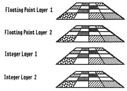
The program handles data in memory in what can be visualized as four matrix levels (Figure 1). Two of the levels are real (floating point) and two are integer. The floating point arrays are of type Float in the C language and on the SUN are 32 bit values, while the integers are stored as 16 bit values. When data are read into an integer level they are rounded off since the original file could contain real numbers.

The reason behind both real and integer value arrays derives both from bookkeeping problems (due to algorithm considerations) and the need to handle operations that are best done in one type or the other. For example,

mathematical calculations are considered to be based on real numbers, whereas Boolean operations are integer. The

modular design of the program allows the memory structure to be augmented (number or type of layers) based on the needs of the researcher. The only limitation would be the amount of memory available on th~ machine and the matrix size of the database.

3.2.3. Operators

Some of the primary fixed operators (operators that perform a set function) will be familiar to anyone who has used Tomlin's MAP program (Table 1). Some major changes

Floating Point layer 1

.A~~

Floating Point loyer

2

Aa~~

Integerlauer 1

~~

Integer loyer 2

A~t~

Figure 1. PROMAP Memory Struture. Each layer represents a two dimensional matrix in which the data are accessible by the row and column coordinates. AI I four layers are accessible at the same time .

Table 1: PROMAP operators

operator Function

MATH Allows maps to be treated as variables in mathematical equations. standard arithmetic operations as well as exponentiation,

trigonometric functions, powers, square roots, and logs are available. Equations can be defined in external files. Global operator.

DRAIN Calculates the relationship between neighboring cells to determine the downhill connections over a terrain surface. Each cell in the output is given the accumulated value of all cells which drain into i t from above. Global operator.

POINT Allows a specified value to be placed in

specified location or locations. The locations can be named individually or in a contiguous block. Changes can be made to cells in an existing matrix without affecting other cells. Local operator.

RECODE Allows specified values in an existing matrix to be given a new value. Global operator.

SLICE Creates an output file by dividing a specified range of values on an input file into equal

intervals, then replacing each input value with a new value indicating the ordinal position of its interval. Global operator.

SPREAD Creates a file by measuring the shortest

distance to each point from any of a selected set of points. Distances -are measured between point centers and represents the accumulated distance from the nearest starting point. Global ·operator.

SCAN The output of this operator is a statistic which represents a neighborhood of some specified size around the current cell. The neighborhood can be either square or circular. Examples of the

statistics are: average, maximum, median, distance. Local operator.

Table 1 continued

Operator Function

MINMAX The output file is created by comparing the values of the input files on a point-by-point basis, and assigning to each point the largest or smallest of its input values. Input files are taken in the order presented and the result of the previous operation is used as the comparison file for the next file in the sequence. Global

operator.

BOOL The operator creates an output file based on a boolean comparison (AND, OR, XOR, NOT)of two or more files. The boolean operation returns zero for false and one for true. Input files are taken in the order presented and the result of the previous operation is used as the comparison file for the next file in the sequence. Global

operator. CROSS

TERRAIN

CLONE

RADIATE

The output file is created by combining the categories of one file with the categories of another file on a point-by-point basis, then assigning a user-specified value to all points of each combination. Combinations for which no output value is specified are automatically assigned a value of zero. The user specified values are supplied as an external file. Global operator.

This operator creates two files based on the input of an elevation file. The files created are SLOPE and ASPECT and the values in the files correspond to the name of the file. An optional file can be created which depicts ridge and drainage areas. Global operator.

This operator is based on SPREAD but takes the value of its starting cell and propagates that value over the surface. Global GFerator.

The output file is a binary representation of the viewsheds of points on a 3D surface. Global operator.

Table 1 continued

operator Function

CELL This operator allow the user to create a new function by supplying an external file which describes how the operator will function. This operator is based on cellular automaton principles and can be programmed to respond to local

conditions. Local operator, programmable. BEHAVE This operator implements the fire behavior

calculations from the DIRECT module of the USFS BEHAVE program. The input and output have been changed to function with the PROMAP system. Global operator.

FIRE The operator creates and output file in which the data represent the predicted spread pattern of a fire from one or more ignition points over some specified period of time. Local operator.

have been made based on the premise that this is a -simulation system and not a GIS. Although PROMAP can

perform all thf~ functions of a GIS it has certain characteristics well suited to ecosystem modeling.

The operators can be one of two types, global or local. A global operator is one in which the operation specified is applied to all cells in the matrix. A local operator is one in which the operation can change from cell to cell. with the exception of a special operator in PROMAP, all operators are global in the same manner as their GIS predecessors.

A second attribute of the operators is that some are designed to make use of information about the surrounding neighborhood. In essence it is desirable in modeling to be able to do three types of operations which involve the neighborhood:

1. accumulate information in a single cell about the neighborhood

2. disseminate information from a single cell to its neighbors

3. inquire as to the status of the neighborhood

Types 1 and 2 always result in some change in status to one or more cells, while type 3 might or might not result in a change.

3.2.4 Mathematical Procedures

PROMAP incorporates two very powerful features of dynamic spatial modeling. The first is a complete mathematical function called MATH. It provides the

capability of doing "map algebra" (Berry, 1987) in a strict mathematical implementation by considering the names of the various data layers as variables, and writing them in the form of an equation. For example, to add two maps together

(on a cell by cell basis for the entire matrix) and then divide by a third, the syntax of this equation would be:

output = ( input1 J, input2 ) / input3

Since the operator understands the rules of precedence (multiplication before division before addition before subtraction) the parentheses are necessary to keep from performing the division before the addition. The operations are carried out on each cell in turn for the entire matrix, thereby adding the values in the cells (1,1) together and then the values of cells (1,2) together, and so on. An option available with the MATH function is the capability to define external files (macros) to be used as input. These files may cc~tain equations that are used often (e.g. the universal soil-loss equation) or that may be too cumbersome to type on the command line. For equations that are used many times in a program with only the input variables

and then supply only the inputs needed for this step. Most mathematical functions are supported by PROMAP, including trigonometric functions, square root, natural logs, and exponentiation.

3.2.5 Programmable operation

The second and most powerful tool is the CELL operator, which is based on the idea of cellular automata. This

operator is programmable by the user through an external script file (ASCII text). It allows the modeler to specify the location of the action (e.g., a specific cell or cells as well as the entire matrix), the influence of the

surrounding neighborhood, and the number of iterations desired. The CELL script file is read into the main PROMAP program and becomes a second program running inside PROMAP while the operator is active. Further work is being done on the CELL operator to provide some type of memory structure. with a form of memory the operator will be able to make decisions on the next action based on past experience

(adaptive learning). This would give the operator the ability to change its initial instruction set based on what it finds in the environment.

3.2.5.1 Example of the CELL operator

The CELL operator provides the basic implementation of cellular automata into the spatially referenced database of a GIS system. As an example of how this operator is

programmed, an example of a CELL script file is shown in Figure 2. The script represents a cellular automaton which uses Conway's Game of Life rules to determine whether a cell is filled (live) or blank (dead) (M. Gardner, 1970). Based on the number of neighbors, a cell will either become live, die, or experience no change in the next generation. In Figure 3 the script file is applied to a particular starting configuration known as a "glidel"". This type of object will move across the matrix over a set of generations. In this particular example the initial state of the system (Figure 3a) has two gliders facing each other. Over the period of six generations the two gliders combine and form a "pond".

zero L11

zero L12

lood LI1 GLIDER

ston

set 1"1=0 toreoch 1 if(HIHO)

set INT = IMT t 1

else endif nfllt if (11) 0) if (1m 3) set 12 = 0 else setl2= 1 endif elst if ( INT = 3 ) RHO ( 11 = 0 ) set 12=1 else sft 12 = 0 endif endif stop loop

til e LI2 GLIOERl

cOPS LI2 L11 loop file L12 GLIDER2 copyL12 LIl loop file L12 GLlDER3 co PO L12 LI1 loop file LI2 6L10ERQ copy L12 LIl loop

fiI e LIZ 6LI OER5

copy L12 LIl loop file 1I2 6LIDER6

Ze~o mat~Ices and load fIle

BegIn global ope~atlon defInition BegIn neighbo~hood loop

Nelghbo~hood Inst~uctions

End of nelghbo~hood loop

Ope~ations based on nelghbo~hood

condItions

End of global ope~ation definition Execute global ope~ation

FIle output. copy mat~ix 2 to mat~lx 1 Repeat as ~equi~ed

FIgu~e 2. CELL Ope~ato~ Sc~Ipt FIle. This Is a sc~lpt

that Implements the Game of Life ~ules. The annotation explains some of the maJo~ st~uctu~es.

a

b

c

_d

e

_f

g

Figu~e 3. Results of Sc~ipt File in Figu~e 2. This

figu~e shows the initial sta~ing configu~ation and the

SECTION "

- 4.1 Modelinq Biophysical system Processes

The desiqn and implementation of PROMAP is only the first step in the development of better ecosystem models. Althouqh many of the restrictions on this type of modeling have been lifted, there still exists the crucial step of how models are constructed.

4.1.1 Representinq the Environment

Consider in this design that the environment is a set of "state" variables. An individual matrix layer in the PROMAP system represents a state variable such as

vegetation, and the individual cells of the matrix represent the current value of the variable at a specific location in the environment. For the model to accurately represent the ecosystem it must be able to start with the state variable at some initial value at time t, and at time t + 1 have changed the state variable to the appropriate value. The specification of how the states change over time is called the transition function. What is needed is to determine how many state variables and what transition functions are

required to model the system.

Holland, et ale (1989) address the problem of levels of approximation in describing systems. They state that

limitations of realistic [modeling] systems, it is

unreasonable to expect ••• models to be isomorphisms in which each unique state of the world maps onto a unique state in the model" (Holland, et.al., 1989, page 31).

Iu their book they consider the design of a layered set of transition functions which they call a quasi-homomorphism or simply a q-morphism. The q-morphism is the mapping of many attributes in the real system through a hierarchical set of transition functions in the model. At the current point in development of a model ecosystem, the q-morphism can be considered in the following manner.

4.1.2 Q-Morphisms in Ecosystem Models

Natural systems are hierarchical structures and as such must be treated in a manner which preserves the hierarchical interactions and properties of such systems. Hierarchical structures exhibit emergent properties which Grobstein

(1973) says are the " ..• result of regulated context II (a

result of interactive influences). He goes on to say that " ... the emergence of new properties in hierarchical systems is closely linked to what we may call the set-superset transition. II This transition can be seen in nature by

observing how climate affects various areas in the

landscape. Higher rainfall coupled with lower temperatures provides a distinctively different floristic composition at

the top of a mountain from a desert area at the base of the mountain. Closer examination reveals further interactions between the plants based on soil conditions, competition for nutrients and light, as well as other factors.

The general tendency when trying to model a system is to describe it mathematically, in other words decompose the system to a set of equations. As Pattee (1973) points out, this causes some problems. He states, " ••. Mathematical descriptions therefore tend to create total decomposition, whereas the essential behavior of real hierarchical systems depends on the partial decomposition of levels. We find then that dynamical systems theory emphasizes holistic, single-level descriptions, avoidance of instabilities, optimization under fixed constraints and artificial isolation of adjacent levels. In contrast to systems theory, hierarchy theory must be formulated to describe at least two levels at a time, it must optimize constraints for a given function, and it must allow interactions between alternative levels." Adopting the q-morphism approach can provide some transition functions which handle the higher level (global) requirements of the system and other transition functions for the lower level (local or