Benchmarking the Selection of the Hidden-layer
Weights in Extreme Learning Machines
Enrique Romero
Department of Computer Science Universitat Polit`ecnica de CatalunyaSpain.
Abstract—Recent years have seen a growing interest in neural networks whose hidden-layer weights are randomly selected, such as Extreme Learning Machines (ELMs). These models are motivated by their ease of development, high computational learning speed and relatively good results. Alternatively, con-structive models that select the hidden-layer weights as a subset of the data have shown superior performance than random-based ones in some cases. In this work, we present a comparison between original ELMs (i.e., ELMs where the hidden-layer weights are selected randomly, that we will call ELM-Random) and a modified version of ELMs where the hidden-layer weights are a subset of the input data (that we will call ELM-Input). We will focus our comparison on the behavior of both strategies for different sizes of the training set and different network sizes. The results on several benchmark data sets for classification problems show that ELM-Input has superior performance than ELM-Random in some cases and similar in the rest. In some cases, this general trend is observed for all sizes of the training set and all network sizes. In other cases, it is mostly observed when the size of the training set is small. Therefore, the strategy of selecting the hidden-layer weights among the data can be considered as a good alternative or complement to the standard random selection for ELMs.
I. INTRODUCTION
Single-hidden-layer feed-forward neural networks (SLFNNs) are well-known approaches for classification and regression problems (see [1], for example) with many practical applications. In these models, the architecture (number of hidden units, activation functions, etc) is usually fixed a priori, whereas the weights are learned during the training process. The most common methods to learn the weights are gradient-based iterative algorithms, such as gradient descent or conjugate gradients, where the gradient is usually computed with the back-propagation algorithm [2]. In these methods, the weights in the hidden and output layers are adjusted simultaneously.
There exist, however, SLFNN models where the learning of the weights is not based on gradient methods. In these models, the weights are typically adjusted in two steps. In the first one, the hidden-layer weights are selected. In the second one, the output-layer weights are computed. The selection of the hidden-layer weights is done heuristically, since the non-linear optimization problem cannot be solved analytically in the general case [3]. The optimal output-layer weights can usually be obtained by solving a linear equations system [4]. One of these methods is Extreme Learning Machines (ELMs, [5], [6]), where the hidden-layer weights are selected
randomly and the output-layer weights are computed with the pseudo-inverse of a matrix that is a function of the data and the hidden-layer weights. Similar ideas to those of ELMs had been previously proposed in [7]–[9], for example. Recent years have seen an important growth of ELMs, mainly because of their ease of development, high computational learning speed and relatively good results. This growth can be seen both in new ELM-based developed models and practical applications. For an extensive review on ELMs, see [10], [11] and references therein.
ELMs are closely related to constructive SLFNNs [12], which are models that construct the network sequentially, usually adding one hidden unit at a time, so that the number of hidden units is also a result of the learning process. Several constructive SLFNNs (see [13]–[16], for example) find the optimal output-layer weights by solving the same linear system than ELMs. In [16], the Error Minimized Extreme Learning Machines (EM-ELMs) is presented, a constructive version of ELMs which results in a faster method with similar generalization performance. In other constructive models [13]– [15], the hidden-layer weights are taken to be a (usually randomly selected) subset of the data. This strategy is called
Input strategy (in contrast to the Random strategy used by ELMs), and its models are named Support Vector Sequential Feed-forward Neural Networks (SV-SFNNs) [17] by their analogy with Support Vector Machines (SVMs) [18], where the support vectors (the hidden-layer weights) are also a subset of the data. The rationale of theInputstrategy is that choosing the hidden-layer weights among the input vectors is more related to the underlying distribution of the data than the
Random strategy, leading to more informative weights (such as prototypes, border points, etc). This idea is also present in vector quantization, since it is guaranteed that densely populated areas of the input space are well represented [19]. In the context of kernel learning, the Inputstrategy can yield better generalization error bounds and results than random Fourier features [20].
The aforementioned models use different strategies to select the hidden-layer weights (Randomfor ELMs and EM-ELMs orInputin SV-SFNNs) and the number of hidden units (fixed
a priori for ELMs or incrementally obtained in EM-ELMs and SV-SFNNs). Some of these strategies have been compared among them and with SVMs. In [7], small-scale experiments with synthetic data are performed comparing both strategies
© 2017 IEEE. Personal use of this material is permitted. Permission from IEEE must be obtained for all other uses, in any current or future media, including reprinting/republishing this material for advertising or promotional purposes,creating new collective works, for resale or redistribution to servers or lists, or reuse of any copyrighted component of this work in other works. DOI: 10.1109/IJCNN.2017.7966043
and back-propagation. In [21], an ELM-based random version of SVMs is described, where the feature space is constructed with random vectors instead of with a subset of the data. Experimental results show that the ELM-based approach is faster than SVMs with comparable results. In [22], ELMs are compared to SVMs. The main conclusions are that ELMs tend to have lower generalization ability than SVMs for smaller samples but generalizes as well as SVMs for larger samples, with lower computational cost (differences in the computational cost are larger for larger-scale problems). SV-SFNNs are compared with SVMs in [17], obtaining similar ac-curacies than SVMs with simpler models. In [23], EM-ELMs are compared with SV-SFNNs, concluding that selecting the hidden-layer weights as a subset of the input data (i.e., with theInputstrategy) outperforms the random selection made by EM-ELMs, with the same computational cost.
These recent results motivate the work presented in this paper. The superior performance of SV-SFNNs over EM-ELMs in [23] may be caused not only by theInputstrategy, but by the combination of the Inputstrategy with a constructive scheme. Except for the preliminary results in [7], to the best of our knowledge it is unknown whether the Input strategy is also able to improve theRandomselection of hidden-layer weights in non-constructive ELMs or not, which is the aim of this paper. More specifically, this work shows a comparison between the original ELMs, that we will call ELM-Random and a modified version of ELMs that we will call ELM-Input. In ELM-Random the hidden-layer weights are selected randomly, as in [6]. ELM-Input can be considered as ELMs with the Inputstrategy, where the hidden-layer weights are a subset of the data. ELM-Input is similar to [17] except for the fixeda priorinumber of hidden units.
An experimental study on several benchmark data sets for classification problems is presented where ELM-Input and ELM-Random are compared in the same conditions. We will focus our comparison on the behavior of both strategies for different sample sizes (by varying the percentage of examples in the training set), as in [22], and different network sizes (by varying the number of hidden units). Since the only difference between the two compared methods is the strategy to select the hidden-layer weights, the results will help to understand whether the use of input data as hidden-layer weights provides any advantage over pure random selection or not. The growing interest in models that randomly select the weights of the hidden units makes this comparison relevant, since it is expected that similar conclusions hold for other ELM-based models.
II. EXTREMELEARNINGMACHINES
The output function of an SLFNN (i.e. a fully connected FNN with a single hidden layer of Nh units) with n input
units and m linear output units can be expressed as a linear combination of simple functions:
fNh(x) =λ0+ Nh
X
i=1
λiϕ(x,ωi, bi) (1)
whereωi∈Rnandbi∈Rare the hidden-layer weights of the hidden units,λi∈Rmare the output-layer weights connecting thei-th hidden unit to themoutput units, ϕis the activation function of the hidden units, ϕ(x,ωi, bi)is the output of the i-th hidden unit with respect to the input x, and λ0 ∈ Rm denotes the bias terms (if any) of the linear output units.
The most common models of SLFNNs are Multi-Layer Perceptrons (MLPs) and Radial Basis Function (RBF) net-works, which mainly differ in the activation function ϕused in equation (1). MLPs typically use any sigmoidal activation function applied to the scalar product of the input and weight vectors (e.g. the logistic function, that will be referred to as a logistic MLP)
ϕ(x,ωi, bi) =
1
1 + exp (−ωi·x−bi)
(2)
The activation function mostly used in RBF networks is the Gaussian function applied to a distance between an input vector and a center, that we will call Gaussian RBF
ϕ(x,ωi, bi) = exp −bi||x−ωi||2/2
, (3)
although many other activation functions can be used to have universal approximation capability.
For logistic MLP units, ωi ∈ Rn is the weight vector connecting the input layer to the i-th hidden unit andbi∈R is the bias of the i-th hidden unit. For Gaussian RBF units,
ωi∈Rn andbi∈R+ are the center and the impact factor of thei-th RBF unit.
For a given set of training examples{(xj,tj)}Lj=1⊂Rn× Rm, if the outputs of the network were equal to the targets, we would have fNh(xj) = Nh X i=1 λiϕ(xj,ωi, bi) =tj, j= 1, . . . , L. (4)
Equation (4) can be written compactly as
Hλ=T (5)
whereHis anL×Nh matrix called the hidden-layer output
matrix of the network (Hji=ϕ(xj,ωi, bi)),λis anNh×m
matrix containing the output-layer weights, andTis anL×m matrix containing the target values in the training set. The output layer biases can be added by including in H a first column with a fixed value of 1 (and increasing Nh by 1).
Normally, the number of training examplesLwill be much greater than the number of hidden units Nh and an exact
solution of (5) cannot be expected. Then, a usual cost function is the sum-of-squares error
E= 1 2 L X j=1 ||fNh(xj)−tj||2= 1 2||Hλ−T|| 2. (6)
It is well known (see [1], for example) that, in order to min-imize E, the optimal output-layer weights can be computed as
ˆ
whereH† is the pseudo-inverse (aka Moore-Penrose general-ized inverse) of the hidden-layer output matrixH. The pseudo-inverse always exists, is unique and, whenHTHis invertible, can be computed as HTH−1HT. The sum-of-squares error of a hidden-layer output matrix can be expressed as
E(H) =1 2||H ˆ λ−T||2= 1 2||HH †T−T||2. (8)
Huang et al. [5] showed that SLFNNs with random weights in the hidden layer have universal approximation capability for many different choices of the activation function, including the ones stated in equations (2) and (3). Based on this result, the ELMs learning algorithm, described in algorithm 1, was proposed [6]. We will call ELM-Random to this algorithm.
Although the original method proposed in [6] only was tested with MLP units, we will extend it to be used with Gaussian RBF units (see section IV-D).
III. EXTREMELEARNINGMACHINES WITH THEINPUT STRATEGY
The algorithm for ELM-Input is described in algorithm 2. The only difference between ELM-Random (algorithm 1) and ELM-Input (algorithm 2) is the selection of the hidden-layer weights: whereas in ELM-Random they are selected in a purely random manner, in ELM-Input they are selected to be a subset of the data. It may be argued that selecting the hidden-layer weights from the data should perform better than selecting them at random, since the former strategy samples the weights from the underlying distribution of the data. This information is lost if the hidden-layer weights are selected without looking at the statistical properties of the data (randomly, for example). However, a random selection of the hidden-layer weights has more flexibility and can obtain weights that, being far away from any data, may be useful for the task.
Algorithm 2 is mainly motivated by the work in [23], where ELMs [16] is compared with SV-SFNNs [17]. EM-ELMs is a constructive version of ELM which results in a faster method with similar generalization performance. SV-SFNNs is a constructive method similar to EM-ELMs with the main difference that the hidden-layer weights are always taken to be a subset of the data. SV-SFNNs are equivalent to the Orthogonal Least Squares Learning algorithm [13], Kernel Matching Pursuit with pre-fitting [14] and SAOCIF with theInputstrategy [15]. The name SV-SFNNs comes from the property shared with SVMs of selecting the hidden-layer weights among the input vectors.
The main conclusion in [23] is that SV-SFNNs outperform EM-ELMs, indicating that the strategy of selecting the hidden-layer weights as a subset of the input data may be better than the random selection made by EM-ELMs. The experiments in this work are devoted to see if that conclusion also holds for the original ELMs.
In [24], a kernel version of ELM is described, where the hidden-layer output matrix H is implicitly defined andHHT is replaced by the kernel matrix. The resulting architecture
Algorithm 1 Algorithm for ELM-Random.
Given a set of training examples {(xj,tj)}Lj=1⊂Rn×Rm, the hidden-layer activation function ϕ(x,ω, b),
andNh number of hidden units fixeda priori
1a. Randomly assign hidden-layer weights{ωi}Nh i=1 from a certain distribution
1b. Randomly assign hidden-layer bias{bi}Ni=1h from a certain distribution
2. Calculate the hidden-layer output matrixH
3. Calculate the output-layer weight matrixλwith (7)
Algorithm 2 Algorithm for ELM-Input.
Given a set of training examples {(xj,tj)}Lj=1⊂Rn×Rm, the hidden-layer activation function ϕ(x,ω, b),
andNh number of hidden units fixeda priori
1a. Randomly assign hidden-layer weights{ωi}Nh i=1 from the data:ωi =xj (ωi1 =6 ωi2 fori16=i2)
1b. Randomly assign hidden-layer bias{bi}Nhi=1 from a certain distribution
2. Calculate the hidden-layer output matrixH
3. Calculate the output-layer weight matrixλwith (7)
is equivalent to a network with L hidden units where every hidden-layer weight is an input example. In [25], the L×L kernel matrix is replaced by a rectangular matrix, whose columns are selected randomly. The resulting algorithm is similar to algorithm 2 with the additional restriction of using kernel functions.
IV. EXPERIMENTS
This section explains the methodology followed in the experiments and discusses the obtained results.
A. Data Sets
The classification benchmark data sets used for the compar-ison were:AustralianCredit,Car Evaluation, Splice-junction
GeneSequences,GermanCredit,Ionosphere, Landsat Satellite (Satimage), Image Segmentation, Sonar and Vehicle Silhou-ettes, that can be found in the UCI repository [26]. A brief description of these data sets is summarized in Table I.
B. Preprocessing
Categorical attributes were codified with a 1-of-C encoding (the p different categories were represented with p input variables, so that only the input variable associated to its category is one, and all others are zero). Subsequently, all the attributes were scaled to mean zero and variance one.
C. Activation Functions
Two different activation functions were used: logistic MLP (2) and Gaussian RBF (3). The main reasons for choosing these activation functions were: i) the logistic MLP activa-tion funcactiva-tion was originally tested in [6], and it has been the most widely used activation function for ELMs; ii) the
TABLE I
DESCRIPTION OF THE BENCHMARK DATA SETS. #INPUTS IS THE NUMBER OF INPUT UNITS OF THE NETWORK,AFTER CODIFYING THE#FEATURES
ORIGINAL FEATURES.
Data Set #Data #Features #Inputs #Classes
Australian 690 14 43 2 Car Evaluation 1728 6 21 4 Gene 3175 60 240 3 Ionosphere 351 34 34 2 Satimage 6435 36 36 6 Segmentation 2310 16 16 7 Sonar 208 60 60 2 Vehicle 846 18 18 4
Gaussian RBF activation function has been the most widely used in models whose hidden-layer weights are a subset of the data, such as SVMs. The parameters bi were set to 0
and 1 for logistic MLP and Gaussian RBF respectively (the comparative results are expected to be independent of the particular selection of these parameters). In order to have more flexibility, a multiplicative positive parameter γ was introduced. Specifically,γ multiplies the scalar productωi·x in logistic MLP units and the distance ||x−ωi||in Gaussian RBF units (γ is equivalent to bi for Gaussian RBF units, but
in this way we can work with the two activation functions in the same manner).
D. Compared Methods
The methods compared were:
• ELM-Random(algorithm 1): ELM with random
hidden-layer weights, i.e. the original method proposed in [6], and extended to Gaussian RBF units with the following particular decisions:
– For MLP units, select the hidden-layer weights uni-formly in[−1,1].
– For RBF units, select the hidden-layer weights uni-formly in[−1,1]and normalize them so as to have the same mean and variance than the training data.
• ELM-Input(algorithm 2): ELM where the hidden-layer weights are selected from the input data as follows:
– Select a random subset of the input examples of size Nh (the number of hidden units).
– For MLP units, normalize them to zero mean and variance one.
– For RBF units, normalize them so as to have the same mean and variance than the training data. Therefore, the only difference between the two compared methods is the selection of the hidden-layer weights: either they are randomly generated (ELM-Random) or randomly obtained from the input patterns (ELM-Input). Clearly, both methods have the same computational cost. This allows to make a fair comparison between them, since they work in the same conditions.
E. Experimental Setting
The aim of the paper is to perform an exploratory analysis of both methods. To this end, we constructed several models
with different number of hidden units and using training sets of different sizes. More particularly, we constructed models with10,20,30,40,50,60,70,80, and90hidden units, each one trained with training sets of sizes 10%, 30%,50%,70%
and90%of the original data set.
In order to get an adequate value for theγparameter, which may be problem-dependent, a search was performed with the following values forγ:0.001,0.002,0.005,0.01,0.02,0.05,
0.1,0.2,0.5,1.0,2.0,4.0,8.0. The same search was performed for all the models, and repeated for every activation function. For every data set and method, therefore, we have a combi-nation of four parameters: the activation function, the number of hidden units, the percentage of examples in the training set and the value ofγ.
F. Model Training and Final Results
For every data set and method, every combination of pa-rameters was trained and tested over30different training-test random partitions of the whole data set. The percentage of training examples was a parameter of the experimental setting, as previously explained.
Let us define a configuration as a tuple composed of five elements: data set, method (ELM-Random or ELM-Input), activation function (logistic MLP or Gaussian RBF), number of hidden units and percentage of examples in the training set. For every configuration, its final result was the lowest average accuracy in the test sets for the different values ofγ.
G. Software
The experiments were performed in Matlab, based on a publicly available version of ELM 1, modified to set the parameters as explained in the previous sections.
H. Results
Tables II to IX show the final results (lowest average test accuracies among allγ) for the two compared methods (ELM-Random and ELM-Input) in the classification data sets studied and the configurations previously described. In the tables, underlined figures show differences between ELM-Random and ELM-Input ranging from2%to5%.Bold figuresindicate differences ranging from 5% to 10%. Differences greater than10% are marked in bold and underlined. The standard deviations (not shown in the tables) were, although slightly lower for ELM-Input, quite similar for both methods. Empty results for ELM-Input correspond to configurations where the number of training examples was less than the number of hidden units (see section IV-E) and therefore the ELM-Input method described in algorithm 2 cannot compute the output-layer weights (missing hidden-output-layer weights could be obtained in different ways, but it was preferred not to change the original algorithm 2).
In summary, the results look similar between ELM-Random and ELM-Input in some cases and a superior performance of ELM-Input can be appreciated in the rest. In our experiments, ELM-Random did not obtain significantly better results than
ELM-Input for any configuration. Although we do not claim that our results are optimal for the tested data sets, they are competitive with the results of other popular state-of-the-art methods (see [27], [28], for example).
In some cases (Gene, Ionosphere andSonar), this general trend is observed for all percentages of examples in the training set and all number of hidden units. For theIonosphere
data set it is more clearly observed for the Gaussian activation function, which is the activation function that obtains better results for this data set. For the Sonar data set, in addition, the differences between the best results of ELM-Random and ELM-Input among all the configurations are quite large.
For the Satimage data set, the differences between ELM-Random and ELM-Input are more marked for small numbers of hidden units. In other cases (Australian, Car Evaluation,
Segmentation and Vehicle), it is mostly observed when the percentage of examples in the training set is small.
Regarding the activation function, the Gaussian RBF obtains usually better results than the logistic MLP, but with no significant difference of behavior between ELM-Random and ELM-Input, except for the Ionosphere and Sonar data sets, where the differences between ELM-Random and ELM-Input are larger for the Gaussian RBF activation function than for the logistic MLP one. Anyway, the results seem to indicate that theInputstrategy is superior to theRandomone independently of the activation function used.
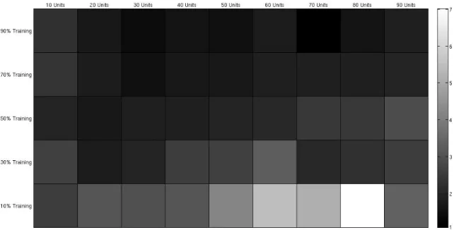
A summary of the differences between ELM-Input and ELM-Random is shown in Figure 1. The gray level of every cell indicates the mean differences between the results of ELM-Input and ELM-Random in tables II to IX: in position
(i, j) we have the mean (over all data sets and the two activation functions tested) of the differences between the results of ELM-Input and ELM-Random for the percentage of training data indicated in row i and number of hidden units indicated in column j. The main conclusion in Figure 1 is that differences are greater when the number of the number of hidden units is small or (more remarkably) when the percentage of examples in the training set is small. Note that all mean differences are greater than1.
In the experiments, the maximum number of hidden units was fixeda priori. In some cases (seeCar Evaluation,Gene,
Satimage or Segmentation for example), it seems clear that better accuracies can be obtained if more hidden units are allowed in the models. The experiments performed with more hidden units (up to500) showed a similar behavior than those of tables II to IX, although the differences decrease when the number of hidden units grows.
V. CONCLUSIONS ANDFUTUREWORK
The main conclusion of this work is that selecting the hidden-layer weights as a subset of the input data experimen-tally outperforms a purely random selection for ELMs with the same computational cost. This is more remarkably observed when there are few examples in the training set, a conclusion that was also observed in [22] when ELMs were compared to SVMs. These results are also consistent with those in [29],
where it is experimentally shown that, for imbalanced data with a small number of examples, the results obtained by ELM-Random are highly variable. Therefore, it seems that when the number of examples is small, selecting the hidden-layer weights among the data should be preferred to selecting them at random. In other cases, it can be considered as a complement to the standard random selection for ELMs, since it could be also possible to construct mixed models, where random andInputweights can be selected in the same network. In the data sets with higher number of variables (see Table I), the aforementioned behavior was also observed for all hidden units and all percentages of examples in the training set. Although this could be justified by the difficulty of finding good hidden-layer weights in a purely random manner, further validation in future studies is needed.
As previously mentioned, one of the reasons that can justify the better performance of ELM-Input over ELM-Random is the fact that choosing the hidden-layer weights among the input vectors is related to the underlying distribution of the data, so that it is expected to obtain better candidates than sampling them randomly (recall that the main objective in this paper is generalization). In this sense, it would be interesting to compare the effect of random and Input weights inde-pendently for approximation and generalization. Intuitively, random weights could be more suitable for approximation since they have more flexibility. For generalization, random weights could lead to models with larger variance that do not compensate the potentially smaller bias.
Although it is expected that similar conclusions hold for other ELM-based models, it should also be the subject of future work.
ACKNOWLEDGMENT
This work was supported in part by the Ministerio de Ciencia e Innovaci´on (MICINN), under project TIN2016-79576-R.
REFERENCES
[1] C. M. Bishop, Neural Networks for Pattern Recognition. Oxford University Press Inc., New York, 1995.
[2] D. E. Rumelhart, G. E. Hinton, and R. J. Williams, “Learning Internal Representations by Error Propagation,” inParallel Distributed Process-ing: Explorations in the Microstructure of Cognition (vol. 1), D. E. Rumelhart and J. L. McClelland, Eds. MIT Press, 1986, pp. 318–362. [3] V. Kurkov´a, “Incremental Approximation by Neural Networks,” in Dealing With Complexity: A Neural Network Approach, M. Karny, K. Warwick, and V. Kurkov´a, Eds. Springer-Verlag, London, 1998, pp. 177–188.
[4] N. I. Achieser,Theory of Approximation. Frederick Ungar Pub. Co., New York, 1956.
[5] G. B. Huang, L. Chen, and C. K. Siew, “Universal Approximation using Incremental Constructive Feedforward Networks with Random Hidden Nodes,” IEEE Transactions on Neural Networks, vol. 17, no. 4, pp. 879–892, 2006.
[6] G. B. Huang, Q. Y. Zhu, and C. K. Siew, “Extreme Learning Machine: Theory and Applications,”Neurocomputing, vol. 70, no. 1-3, pp. 489– 501, 2006.
[7] W. Schmidt, M. Kraaijveld, and R. Duin, “Feedforward Neural Networks with Random Weights,” inIAPR International Conference on Pattern Recognition Methodology and Systems, 1992, pp. 1–4.
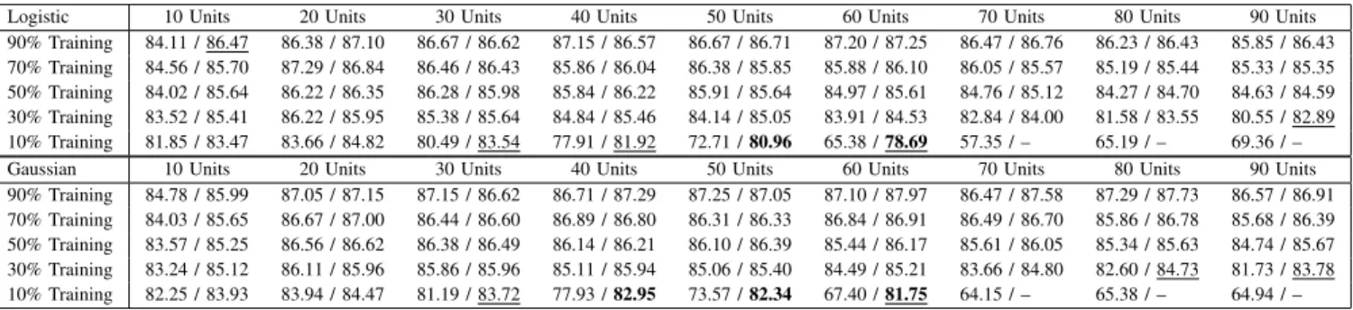
TABLE II
FINAL RESULTS FOR THEAustralianDATA SET AND THE LOGISTIC(TOP)ANDGAUSSIAN(BOTTOM)ACTIVATION FUNCTIONS(LEFT/RIGHT: ELM-RANDOM/ELM-INPUT)
Logistic 10 Units 20 Units 30 Units 40 Units 50 Units 60 Units 70 Units 80 Units 90 Units 90% Training 84.11 / 86.47 86.38 / 87.10 86.67 / 86.62 87.15 / 86.57 86.67 / 86.71 87.20 / 87.25 86.47 / 86.76 86.23 / 86.43 85.85 / 86.43 70% Training 84.56 / 85.70 87.29 / 86.84 86.46 / 86.43 85.86 / 86.04 86.38 / 85.85 85.88 / 86.10 86.05 / 85.57 85.19 / 85.44 85.33 / 85.35 50% Training 84.02 / 85.64 86.22 / 86.35 86.28 / 85.98 85.84 / 86.22 85.91 / 85.64 84.97 / 85.61 84.76 / 85.12 84.27 / 84.70 84.63 / 84.59 30% Training 83.52 / 85.41 86.22 / 85.95 85.38 / 85.64 84.84 / 85.46 84.14 / 85.05 83.91 / 84.53 82.84 / 84.00 81.58 / 83.55 80.55 / 82.89 10% Training 81.85 / 83.47 83.66 / 84.82 80.49 / 83.54 77.91 / 81.92 72.71 /80.96 65.38 /78.69 57.35 / – 65.19 / – 69.36 / – Gaussian 10 Units 20 Units 30 Units 40 Units 50 Units 60 Units 70 Units 80 Units 90 Units 90% Training 84.78 / 85.99 87.05 / 87.15 87.15 / 86.62 86.71 / 87.29 87.25 / 87.05 87.10 / 87.97 86.47 / 87.58 87.29 / 87.73 86.57 / 86.91 70% Training 84.03 / 85.65 86.67 / 87.00 86.44 / 86.60 86.89 / 86.80 86.31 / 86.33 86.84 / 86.91 86.49 / 86.70 85.86 / 86.78 85.68 / 86.39 50% Training 83.57 / 85.25 86.56 / 86.62 86.38 / 86.49 86.14 / 86.21 86.10 / 86.39 85.44 / 86.17 85.61 / 86.05 85.34 / 85.63 84.74 / 85.67 30% Training 83.24 / 85.12 86.11 / 85.96 85.86 / 85.96 85.11 / 85.94 85.06 / 85.40 84.49 / 85.21 83.66 / 84.80 82.60 / 84.73 81.73 / 83.78 10% Training 82.25 / 83.93 83.94 / 84.47 81.19 / 83.72 77.93 /82.95 73.57 /82.34 67.40 /81.75 64.15 / – 65.38 / – 64.94 / – TABLE III
FINAL RESULTS FOR THECar EvaluationDATA SET AND THE LOGISTIC(TOP)ANDGAUSSIAN(BOTTOM)ACTIVATION FUNCTIONS(LEFT/RIGHT: ELM-RANDOM/ELM-INPUT)
Logistic 10 Units 20 Units 30 Units 40 Units 50 Units 60 Units 70 Units 80 Units 90 Units 90% Training 75.99 / 75.97 84.76 / 84.39 84.55 / 84.51 84.20 / 84.78 84.22 / 84.45 84.43 / 84.51 84.82 / 84.82 84.70 / 85.51 85.03 / 84.99 70% Training 75.22 / 75.43 84.26 / 84.53 84.01 / 84.17 83.87 / 84.34 84.02 / 84.53 84.18 / 84.66 84.23 / 84.33 84.62 / 84.73 84.48 / 84.86 50% Training 75.45 / 74.79 83.95 / 83.82 83.69 / 83.92 83.44 / 83.90 83.55 / 84.12 83.72 / 84.04 83.76 / 84.32 83.84 / 84.39 84.08 / 84.69 30% Training 75.02 / 75.37 83.43 / 83.53 82.87 / 83.56 82.70 / 83.34 82.59 / 83.36 82.41 / 83.79 82.44 / 83.63 82.65 / 84.14 82.55 / 84.09 10% Training 74.46 / 74.85 81.08 / 81.36 80.06 / 81.76 79.10 / 82.03 78.07 / 82.08 77.03 /82.14 75.69 /82.24 75.33 /82.22 73.40 /82.52
Gaussian 10 Units 20 Units 30 Units 40 Units 50 Units 60 Units 70 Units 80 Units 90 Units 90% Training 75.61 / 75.24 84.24 / 83.80 83.78 / 84.43 84.76 / 84.76 85.38 / 85.09 86.84 / 86.86 87.80 / 87.34 88.59 / 88.15 89.85 / 89.85 70% Training 74.92 / 74.75 83.79 / 83.71 84.03 / 83.85 84.74 / 84.31 85.49 / 85.08 86.06 / 86.38 87.61 / 87.06 88.54 / 88.26 89.65 / 89.65 50% Training 74.94 / 74.94 83.88 / 83.49 83.58 / 83.58 84.22 / 84.06 84.85 / 85.06 86.13 / 85.71 86.75 / 86.79 88.00 / 87.75 89.08 / 88.96 30% Training 74.54 / 74.70 83.13 / 83.14 83.23 / 83.02 83.51 / 83.66 84.32 / 84.35 84.99 / 85.31 86.16 / 86.31 87.07 / 87.05 88.39 / 88.33 10% Training 74.16 / 74.70 80.96 / 80.99 80.39 / 81.78 80.88 / 81.59 80.94 / 82.42 80.90 / 82.71 81.45 / 82.81 81.22 / 83.20 81.23 / 83.48 TABLE IV
FINAL RESULTS FOR THEGeneDATA SET AND THE LOGISTIC(TOP)ANDGAUSSIAN(BOTTOM)ACTIVATION FUNCTIONS(LEFT/RIGHT: ELM-RANDOM/ELM-INPUT)
Logistic 10 Units 20 Units 30 Units 40 Units 50 Units 60 Units 70 Units 80 Units 90 Units 90% Training 57.18 / 59.95 63.14 /68.48 69.18 / 74.03 72.64 /78.55 77.00 / 81.83 79.78 /85.45 82.59 / 86.26 84.75 / 88.03 86.82 / 90.07 70% Training 56.75 / 59.69 63.10 / 67.95 68.45 /74.04 73.22 / 78.15 76.53 /82.06 79.17 /84.24 82.07 / 86.35 84.28 / 88.23 86.49 / 89.33 50% Training 57.08 / 59.62 62.71 / 67.47 68.06 /74.19 73.16 / 77.93 76.10 /81.20 79.29 / 83.96 81.54 / 86.26 83.94 / 87.33 85.97 / 88.97 30% Training 56.66 / 59.94 62.99 / 67.02 67.74 /72.89 71.49 /77.30 74.97 /80.98 78.22 / 83.16 80.74 / 85.07 83.21 / 86.95 84.48 / 87.96 10% Training 55.58 / 58.41 61.08 / 65.46 65.39 /70.94 68.42 /74.11 71.24 /77.26 73.87 / 78.72 75.82 / 80.46 77.15 / 81.81 78.34 / 82.41 Gaussian 10 Units 20 Units 30 Units 40 Units 50 Units 60 Units 70 Units 80 Units 90 Units 90% Training 57.74 / 60.72 64.29 /69.97 69.79 /75.05 74.30 /79.50 78.13 / 82.24 81.69 / 85.05 84.52 / 87.53 85.66 / 89.10 87.71 / 90.38 70% Training 57.51 / 60.57 64.36 / 69.32 69.76 /75.33 73.99 /78.99 77.63 / 82.53 81.02 / 85.22 83.35 / 87.19 85.33 / 88.75 87.45 / 89.97 50% Training 57.94 / 60.67 64.33 / 68.67 69.74 /75.44 73.63 /79.01 77.55 /82.72 80.21 / 84.62 82.86 / 86.75 85.02 / 88.18 86.93 / 89.61 30% Training 56.96 / 60.92 63.69 / 68.39 68.92 /74.04 73.76 / 78.06 76.72 / 81.47 79.20 / 84.04 82.23 / 85.96 83.98 / 87.34 85.94 / 88.50 10% Training 56.28 / 59.91 61.72 / 66.58 66.55 /72.24 69.94 /75.83 72.52 /78.73 75.36 / 80.33 76.75 / 81.74 78.53 / 82.89 79.42 / 83.48 TABLE V
FINAL RESULTS FOR THEIonosphereDATA SET AND THE LOGISTIC(TOP)ANDGAUSSIAN(BOTTOM)ACTIVATION FUNCTIONS(LEFT/RIGHT: ELM-RANDOM/ELM-INPUT)
Logistic 10 Units 20 Units 30 Units 40 Units 50 Units 60 Units 70 Units 80 Units 90 Units 90% Training 82.78 / 86.76 86.94 / 88.15 88.43 / 87.78 87.50 / 88.15 87.50 / 87.59 86.20 / 87.41 88.15 / 87.50 87.59 / 86.94 86.11 / 88.43 70% Training 82.80 / 85.82 85.82 / 87.17 86.79 / 87.55 86.07 / 86.70 85.72 / 86.79 85.57 / 86.29 85.16 / 86.51 84.37 / 86.32 83.68 / 85.47 50% Training 83.43 / 85.08 85.30 / 86.88 86.16 / 86.25 85.55 / 86.10 84.53 / 85.53 84.49 / 85.27 83.11 / 84.79 82.27 / 83.98 81.40 / 83.03 30% Training 82.66 / 84.84 84.31 / 85.54 84.12 / 84.72 82.59 / 83.04 81.15 / 82.10 80.22 / 81.79 78.17 / 80.64 76.41 / 80.20 75.73 / 79.62 10% Training 78.65 / 82.45 79.07 / 79.50 73.57 / 75.01 73.60 / – 75.81 / – 78.23 / – 79.62 / – 79.28 / – 80.13 / – Gaussian 10 Units 20 Units 30 Units 40 Units 50 Units 60 Units 70 Units 80 Units 90 Units 90% Training 82.41 / 86.20 87.13 / 88.06 87.31 / 88.98 88.98 / 91.02 88.43 / 91.20 89.17 / 90.65 88.70 / 90.65 87.59 / 92.13 87.59 / 90.74 70% Training 82.99 / 85.82 86.16 / 89.06 87.74 / 88.52 87.52 / 89.75 87.55 / 89.87 87.01 / 90.44 87.67 / 89.84 86.73 / 90.09 87.26 / 90.41 50% Training 82.80 / 85.51 85.78 / 87.48 86.52 / 88.43 86.10 / 88.71 85.63 / 88.62 85.19 / 89.13 84.70 / 88.60 83.84 /89.00 82.88 /88.35
30% Training 82.97 / 84.86 84.35 / 86.56 84.42 / 86.22 83.41 / 86.49 82.53 / 86.41 82.15 / 86.48 80.08 /86.22 78.16 /85.85 74.81 /86.44
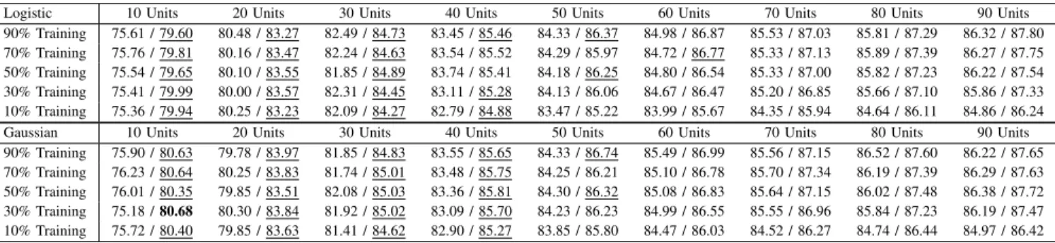
TABLE VI
FINAL RESULTS FOR THESatimageDATA SET AND THE LOGISTIC(TOP)ANDGAUSSIAN(BOTTOM)ACTIVATION FUNCTIONS(LEFT/RIGHT: ELM-RANDOM/ELM-INPUT)
Logistic 10 Units 20 Units 30 Units 40 Units 50 Units 60 Units 70 Units 80 Units 90 Units 90% Training 75.61 / 79.60 80.48 / 83.27 82.49 / 84.73 83.45 / 85.46 84.33 / 86.37 84.98 / 86.87 85.53 / 87.03 85.81 / 87.29 86.32 / 87.80 70% Training 75.76 / 79.81 80.16 / 83.47 82.24 / 84.63 83.54 / 85.52 84.29 / 85.97 84.72 / 86.77 85.33 / 87.13 85.89 / 87.39 86.27 / 87.75 50% Training 75.54 / 79.65 80.10 / 83.55 81.85 / 84.89 83.74 / 85.41 84.18 / 86.25 84.80 / 86.54 85.33 / 87.00 85.82 / 87.23 86.22 / 87.54 30% Training 75.41 / 79.99 80.00 / 83.57 82.31 / 84.45 83.11 / 85.28 84.13 / 86.06 84.67 / 86.47 85.20 / 86.85 85.66 / 87.10 85.86 / 87.33 10% Training 75.36 / 79.94 80.25 / 83.23 82.09 / 84.27 82.79 / 84.88 83.47 / 85.22 83.99 / 85.67 84.35 / 85.94 84.64 / 86.11 84.86 / 86.24 Gaussian 10 Units 20 Units 30 Units 40 Units 50 Units 60 Units 70 Units 80 Units 90 Units 90% Training 75.90 / 80.63 79.78 / 83.97 81.85 / 84.83 83.55 / 85.65 84.33 / 86.74 85.49 / 86.99 85.56 / 87.15 86.52 / 87.60 86.22 / 87.65 70% Training 76.23 / 80.64 80.25 / 83.83 81.74 / 85.01 83.48 / 85.75 84.25 / 86.21 85.10 / 86.78 85.70 / 87.34 86.19 / 87.39 86.29 / 87.63 50% Training 76.01 / 80.35 79.85 / 83.51 82.08 / 85.03 83.36 / 85.81 84.30 / 86.32 85.08 / 86.83 85.64 / 87.15 86.02 / 87.48 86.38 / 87.72 30% Training 75.18 /80.68 80.30 / 83.84 81.92 / 85.02 83.09 / 85.70 84.23 / 86.23 84.99 / 86.55 85.55 / 86.96 85.84 / 87.23 86.19 / 87.47 10% Training 75.72 / 80.40 79.85 / 83.63 81.41 / 84.62 82.90 / 85.27 83.85 / 85.80 84.47 / 86.03 84.52 / 86.27 84.74 / 86.44 84.97 / 86.42 TABLE VII
FINAL RESULTS FOR THESegmentationDATA SET AND THE LOGISTIC(TOP)ANDGAUSSIAN(BOTTOM)ACTIVATION FUNCTIONS(LEFT/RIGHT: ELM-RANDOM/ELM-INPUT)
Logistic 10 Units 20 Units 30 Units 40 Units 50 Units 60 Units 70 Units 80 Units 90 Units 90% Training 75.92 / 76.72 82.73 / 84.30 84.04 / 85.05 85.17 / 86.18 85.32 / 86.62 86.15 / 87.85 86.09 / 88.04 87.40 / 88.53 87.16 / 88.74 70% Training 76.43 / 77.50 82.68 / 84.02 83.75 / 85.32 84.67 / 86.12 85.11 / 86.50 85.87 / 86.90 86.43 / 87.68 86.53 / 87.77 87.45 / 88.42 50% Training 75.70 / 76.15 82.09 / 83.91 83.84 / 85.18 84.27 / 85.75 85.02 / 86.22 85.63 / 86.85 86.01 / 87.49 86.58 / 87.96 86.99 / 88.01 30% Training 75.78 / 76.30 81.86 / 83.39 83.01 / 84.85 83.68 / 85.34 84.29 / 85.60 85.03 / 86.11 85.57 / 87.07 85.69 / 87.17 86.23 / 87.36 10% Training 75.78 / 75.91 80.39 / 82.01 81.35 / 82.32 81.66 / 83.29 81.78 / 84.10 81.66 / 83.64 81.59 / 83.88 81.37 / 83.73 81.34 / 82.70 Gaussian 10 Units 20 Units 30 Units 40 Units 50 Units 60 Units 70 Units 80 Units 90 Units 90% Training 77.53 / 77.14 83.81 / 85.02 85.21 / 86.45 85.86 / 87.53 86.98 / 88.57 87.32 / 89.38 88.18 / 89.37 88.24 / 89.71 89.16 / 89.96 70% Training 78.32 / 78.45 83.60 / 84.48 84.98 / 86.15 85.73 / 87.15 86.65 / 87.94 87.37 / 88.76 87.65 / 89.11 88.30 / 89.50 88.46 / 89.88 50% Training 77.66 / 77.58 83.59 / 84.48 84.80 / 86.15 85.58 / 86.91 86.66 / 87.89 86.95 / 88.63 87.33 / 88.87 87.81 / 89.29 88.18 / 89.58 30% Training 76.98 / 78.88 83.26 / 84.08 84.25 / 85.60 85.08 / 86.71 85.77 / 87.64 86.59 / 88.15 86.85 / 88.61 86.96 / 88.71 87.26 / 89.15 10% Training 76.95 / 76.83 81.63 / 82.98 82.83 / 84.38 83.38 / 84.69 83.92 / 85.54 83.49 / 85.89 83.11 / 85.69 82.74 / 85.42 82.08 / 85.13 TABLE VIII
FINAL RESULTS FOR THESonarDATA SET AND THE LOGISTIC(TOP)ANDGAUSSIAN(BOTTOM)ACTIVATION FUNCTIONS(LEFT/RIGHT: ELM-RANDOM/ELM-INPUT)
Logistic 10 Units 20 Units 30 Units 40 Units 50 Units 60 Units 70 Units 80 Units 90 Units 90% Training 72.70 / 76.51 74.13 / 76.35 77.14 / 77.30 77.62 / 78.41 78.10 / 78.41 76.51 / 78.10 78.10 / 76.51 76.03 / 78.41 74.92 / 77.94 70% Training 70.38 /75.86 75.11 / 75.54 74.84 / 75.16 74.73 / 76.02 75.11 / 74.68 73.98 / 75.00 74.41 / 76.40 73.23 / 75.00 71.99 / 75.11 50% Training 69.81 / 74.16 72.63 / 75.43 72.41 / 74.16 72.57 / 73.24 71.11 / 72.98 70.92 / 72.13 68.63 / 71.37 66.83 / 69.56 64.16 /70.73
30% Training 67.17 /73.29 70.57 / 73.04 68.86 / 70.73 66.58 / 68.63 64.16 / 64.91 58.36 / 59.95 60.59 / – 64.25 / – 65.73 / – 10% Training 64.83 / 68.95 57.29 /67.79 64.17 / – 65.60 / – 65.86 / – 66.77 / – 67.81 / – 68.82 / – 67.81 / – Gaussian 10 Units 20 Units 30 Units 40 Units 50 Units 60 Units 70 Units 80 Units 90 Units 90% Training 71.11 / 75.08 76.98 / 79.68 76.67 / 80.95 76.83 / 81.43 78.73 / 81.75 79.37 /84.76 79.37 / 83.33 76.83 /85.40 77.78 /85.56 70% Training 71.40 / 75.16 73.71 / 77.53 76.34 / 79.35 75.86 /81.08 75.75 /83.01 76.02 /82.96 75.54 /85.05 75.97 /84.73 73.71 /85.43 50% Training 69.11 / 73.84 73.14 / 76.51 72.79 /77.87 72.76 /80.48 73.14 /80.29 71.81 /81.49 70.98 /83.75 68.48 /84.25 65.59 /84.60 30% Training 67.92 /73.36 70.41 /75.91 68.74 /76.62 66.28 /79.79 64.63 /79.34 57.74 /81.85 62.05 / – 64.43 / – 64.06 / – 10% Training 63.16 /71.23 57.36 /71.30 62.41 / – 64.31 / – 65.72 / – 65.99 / – 66.19 / – 66.76 / – 66.49 / – TABLE IX
FINAL RESULTS FOR THEVehicleDATA SET AND THE LOGISTIC(TOP)ANDGAUSSIAN(BOTTOM)ACTIVATION FUNCTIONS(LEFT/RIGHT: ELM-RANDOM/ELM-INPUT)
Logistic 10 Units 20 Units 30 Units 40 Units 50 Units 60 Units 70 Units 80 Units 90 Units 90% Training 66.00 / 67.80 77.61 / 77.84 78.75 / 78.55 79.37 / 79.37 79.06 / 79.88 79.22 / 80.51 79.80 / 80.59 80.47 / 80.31 79.61 / 80.59 70% Training 65.22 / 67.61 76.51 / 77.56 78.39 / 78.43 78.50 / 79.20 78.75 / 79.00 78.83 / 79.16 78.54 / 79.16 78.92 / 79.66 79.06 / 79.37 50% Training 65.57 / 66.42 76.92 / 76.82 77.52 / 77.78 78.16 / 78.40 77.76 / 78.40 77.87 / 78.07 77.73 / 78.54 77.78 / 78.22 77.20 / 78.18 30% Training 63.74 / 65.88 76.12 / 76.28 76.71 / 76.66 76.17 / 76.69 75.63 / 76.82 75.34 / 76.54 74.80 / 76.11 74.74 / 75.91 74.12 / 75.27 10% Training 61.63 / 63.39 72.41 / 72.68 70.27 / 71.98 67.45 / 70.95 64.53 / 69.00 60.43 /67.19 53.61 /65.83 42.70 /63.94 40.88 / – Gaussian 10 Units 20 Units 30 Units 40 Units 50 Units 60 Units 70 Units 80 Units 90 Units 90% Training 66.59 / 66.59 78.08 / 77.45 78.39 / 78.75 80.63 / 79.69 81.33 / 81.57 82.43 / 82.24 83.76 / 82.82 83.80 / 82.24 83.69 / 83.61 70% Training 65.60 / 67.56 77.15 / 76.63 78.98 / 78.70 79.54 / 79.65 80.67 / 80.62 81.55 / 82.43 81.89 / 82.43 82.73 / 82.15 83.04 / 82.85 50% Training 64.89 / 65.97 76.78 / 75.91 78.36 / 78.28 78.51 / 78.81 79.90 / 79.86 80.33 / 80.83 80.75 / 80.86 81.45 / 81.34 81.46 / 81.71 30% Training 65.03 / 65.79 76.16 / 75.23 77.05 / 77.25 77.66 / 78.31 78.43 / 78.51 78.59 / 78.92 78.70 / 79.05 79.26 / 79.01 79.04 / 79.39 10% Training 62.30 / 63.20 72.64 / 72.30 71.56 / 72.50 70.74 / 72.69 69.01 / 72.23 63.89 /71.12 57.04 /69.92 46.91 /69.70 42.89 / –
Fig. 1. Mean differences between ELM-Random and ELM-Input for the different data set and activation functions (see text for details).
[8] B. Igelnik and Y. H. Pao, “Stochastic Choice of Basis Functions in Adaptive Function Approximation and the Functional-link Net,”IEEE Transactions on Neural Networks, vol. 6, no. 6, pp. 1320–1329, 1995. [9] E. Romero and R. Alqu´ezar, “A New Incremental Method for Function
Approximation using Feed-forward Neural Networks,” inInternational Joint Conference on Neural Networks, vol. 2, 2002, pp. 1968–1973. [10] G. B. Huang, D. H. Wang, and Y. Lan, “Extreme Learning Machines:
a Survey,”International Journal of Machine Learning and Cybernetics, vol. 2, pp. 107–122, 2011.
[11] G. Huang, G. B. Huang, S. Song, and K. You, “Trends in Extreme Learning Machines: A Review,”Neural Networks, vol. 61, pp. 32–48, 2015.
[12] T. Y. Kwok and D. Y. Yeung, “Constructive Algorithms for Structure Learning in Feedforward Neural Networks for Regression Problems,” IEEE Transactions on Neural Networks, vol. 8, no. 3, pp. 630–645, 1997.
[13] S. Chen, C. F. N. Cowan, and P. M. Grant, “Orthogonal Least Squares Learning Algorithm for Radial Basis Function Networks,”IEEE Trans-actions on Neural Networks, vol. 2, no. 2, pp. 302–309, 1991. [14] P. Vincent and Y. Bengio, “Kernel Matching Pursuit,”Machine Learning,
vol. 48, no. 1-3, pp. 165–187, 2002.
[15] E. Romero and R. Alqu´ezar, “A Sequential Algorithm for Feed-forward Neural Networks with Optimal Coefficients and Interacting Frequen-cies,”Neurocomputing, vol. 69, no. 13-15, pp. 1540–1552, 2006. [16] G. Feng, G. B. Huang, Q. Lin, and R. Gay, “Error Minimized Extreme
Learning Machine with Growth of Hidden Nodes and Incremental Learning,”IEEE Transactions on Neural Networks, vol. 20, no. 8, pp. 1352–1357, 2009.
[17] E. Romero and D. Toppo, “Comparing Support Vector Machines and Feed-forward Neural Networks with Similar Hidden-layer Weights,” IEEE Transactions on Neural Networks, vol. 18, no. 3, pp. 959–963, 2007.
[18] V. N. Vapnik, The Nature of Statistical Learning Theory. Springer-Verlag, NY, 1995.
[19] A. Coates and A. Y. Ng, “The Importance of Encoding versus Training with Sparse Coding and Vector Quantization,” inInternational Confer-ence on Machine Learning, 2011, pp. 921–928.
[20] T. Yang, Y. F. Li, M. Mahdavi, R. Jin, and Z. H. Zhou, “Nystr¨om Method vs Random Fourier Features: A Theoretical and Empirical Comparison,”
inAdvances in Neural Information Processing Systems, vol. 25, 2012, pp. 476–484.
[21] B. Fr´enay and M. Verleysen, “Using SVMs with Randomised Feature Spaces: An Extreme Learning Approach,” inEuropean Symposium on Artificial Neural Networks, 2010, pp. 315–320.
[22] X. Liu, C. Gao, and P. Li, “A Comparative Analysis of Support Vector Machines and Extreme Learning Machines,”Neural Networks, vol. 33, pp. 58–66, 2012.
[23] E. Romero and R. Alqu´ezar, “Comparing Error Minimized Extreme Learning Machines and Support Vector Sequential Feed-forward Neural Networks,”Neural Networks, vol. 25, pp. 122–129, 2012.
[24] G. B. Huang, H. Zhou, X. Ding, and R. Zhang, “Extreme Learning Ma-chine for Regression and Multiclass Classification,”IEEE Transactions on Systems, Man and Cybernetics, part B: Cybernetics, vol. 42, no. 2, pp. 513–529, 2012.
[25] W. Deng, Q. Zheng, and K. Zhang, “Reduced Extreme Learning Ma-chine,” inInternational Conference on Computer Recognition Systems, 2013, pp. 63–69.
[26] A. Asuncion and D. J. Newman, “UCI machine learning repository,” 2007, university of California, Irvine, School of Information and Com-puter Science. http://www.ics.uci.edu/∼mlearn/MLRepository.html. [27] T. Van Gestel, B. Suykens, J. A. K. Baesens, S. Viane, J.
Van-thienen, G. Ded ene, B. De Moor, and J. Vandewalle, “Benchmarking Least Squares Support Vector Machine Classifiers,”Machine Learning, vol. 54, no. 1, pp. 5–32, 2004.
[28] W. Duch, N. Jankowski, and T. Maszczyk, “Make it Cheap: Learning withO(nd)Complexity,” inInternational Joint Conference on Neural Networks, 2012, pp. 1–4.
[29] S. Suresh, S. Saraswathi, and N. Sundararajan, “Performance En-hancement of Extreme Learning Machines for Multi-Category Sparse Data Classification Problems,” Engineering Applications of Artificial Intelligence, vol. 23, pp. 1149–1157, 2010.