A Data Science Methodology Based on Machine
Learning Algorithms for Flood Severity Prediction
Mohammed Khalaf1,2, Abir Jaafar Hussain1, Dhiya Al-Jumeily1, Thar Baker1, Robert Keight1, Paulo Lisboa1, Ala S. Al Kafri1,
Paul Fergus1
1Faculty of Engineering and Technology, Liverpool John Moores University, Byrom Street, Liverpool, L3 3AF, UK
2 University of Anbar, Ministry of Higher Education and Scientific Research, Bagdad, Al-Rusafa Region, Iraq
[email protected], {a.hussain, d.aljumeily, P.Fergus, T.M.Baker, P.lisboa}@ljmu.ac.uk, [email protected].
Abstract —In this paper, a novel application of machine
learning algorithms including Neural Network architecture is presented for the prediction of flood severity. Floods are considered natural disasters that cause wide scale devastation to areas affected. The phenomenon of flooding is commonly caused by runoff from rivers and precipitation, specifically during periods of extremely high rainfall. Due to the concerns surrounding global warming and extreme ecological effects, flooding is considered a serious problem that has a negative impact on infrastructure and humankind. This paper attempts to address the issue of flood mitigation through the presentation of a new flood dataset, comprising 2000 annotated flood events, where the severity of the outcome is categorised according to 3 target classes, demonstrating the respective severities of floods. The paper also presents various types of machine learning algorithms for predicting flood severity and classifying outcomes into three classes, normal, abnormal, and high-risk floods. Extensive research indicates that artificial intelligence algorithms could produce enhancement when utilised for the pre-processing of flood data. These approaches helped in acquiring better accuracy in the classification techniques. Neural network architectures generally produce good outcomes in many applications, however, our experiments results illustrated that random forest classifier yields the optimal results in comparison with the benchmarked models.
Keywords —Machine learning approaches; Flood datasets; Big data;; Receiver operating characteristic (ROC); Performance evaluations; Accuracy, The Area Under Curve (AUC);
I. INTRODUCTION
Flooding is considered a common natural phenomenon in the globe, causing economic damage, property, and most importantly to human lives. In order to prevent the devastating effects of floods before such events occur, early warning for people to evacuate in the nearby areas can be effective in saving lives and to prevent disasters. There is a significant need for collaboration and the sharing of experience among countries around the world, such as to mitigate the impact of flood events before they proceed to a serious condition. This long-standing natural disaster phenomenon cannot be escaped but suitable pre-alarming and managing systems can mitigate the severity of its impact. As a result, inhabitants who are located within known
flood zones are exposed to the prospect of repeat flooding events each year. To determine the river water levels, machine learning models offer the promise of an advanced predictive solution. Machine learning algorithms have been widely used to fulfil various classification requirements [1]. These models have substantial benefits for classifying datasets due to their computational efficiency, flexibility, and intuitive simplicity. Several machine learning techniques have been selected to carry out the classification of our research, including Artificial Neural Network (ANN) architectures, in conjunction with the Levenberg-Marquardt learning algorithm (LEVNN) [2, 3], Support Vector Machine (SVM) [4], and Random Forest Classifiers (RFC) [5].
The initial case study is to investigate the potential of an empirical dataset for the classification of flood severity, using various machine learning algorithms to get better accuracy. In our study, the datasets integrate various types of features, which are important to distinguish the severity of flood. For instance, water level, duration during day, and Magnitude. The datasets were based on time series and were classified into three classes. Class one belongs to the normal flood, class two refers to the abnormal flood, while class three represents the high-risk level. Our simulation results indicated that support vector machines produced inferior results when compared to random forest model. The results also indicated that of the neural network models tested, the LEVNN and RF performed significantly better using the performance measures examined.
The reminder of this paper is organized as follows. Section II illustrates related work, while section III discusses the classification of flood data. Algorithms are described in Section IV. The methodology is introduced in Section V, followed by the presentation of our results in section VI. In Section VIII, We presented the conclusions and future work.
II.RELATED WORKS
Intelligent systems technology provides a set of new primitive operations within the environmental domain and has become an increasingly important constituent in the advancement of many application areas. Significant developments have been achieved with the early warning systems for heavy excessive rainfall, when rivers overflow, dams or levees break [7]. Many researches have proposed various types of solution in order to solve problems that are related with flood natural disaster of small and large areas with various degree of success in obtaining optimum results. Duncan et al [8] proposed a Machine Learning-Based Early Warning
System for Urban Flood Management. It works with drainage systems and the use of overall rainfall data concurrently, in order to predict flooding of multiple urban zones using a single multi-output ANN. In their study, there are three input time-series used: cumulative rainfall (mm), rainfall intensity (mm/hour), and the new antecedent precipitation index value (metres). The principal goal of their research is to find the true positive rates for sensitivity analysis. The research findings show that the predictive ability of the system depends on actual rainfall.
Li et al [6] established an ANN model to predict the trend of storm flooding in China. The ANN model was used to predict the storm flooding and built to simulate the historical storm surge at typhoon periods. The results showed that the ANN model provides stronger results than other models for flood prediction.
Xia, and Rao [7] designed a new application that utilised a Basis Prediction artificial (BP- artificial) neural network model to predict the flood level in lakes, rivers, and reservoirs. The errors between predicted and actual value are feedback in the process of learning. Their research primarily compares the data calculated by the model to actual monitoring data from the monitoring station from the city of Chaoan; with the result showing that the algorithm can obtain a better prediction. They compared the values calculated by the algorithm to actual monitoring data from monitoring control centre; the result shows that the BP- artificial neural network model can achieve better prediction in terms of accuracy and credibility, in comparison with other neural network architectures.
Our extensive research indicates that no studies have been applied for classifying flood datasets for the provision of providing accurate decision to the flood control system, based on previous datasets and flood severity. This study introduces the novel application of random forest and other machine learning techniques, which focus on flood data collection based on severity features.
III. CLASSIFICATION
In recent times, machine learning models have been designed and used to deal with high-dimensional illustrations through the unification of supervised learning algorithms and feature selection [8, 9]. The classification techniques comprise the following: a number of attributes or features represents each object in a dataset, where such features in combination may be used to infer one or more classes to which a given object [10]. The features can be assembled into input vector x. A number of previous objects (training set), each involving vectors of feature values and the label of the correct class will be provided to the classifier. The principal aim of the learning process is to establish how to extract the most useful information from the labelled data. There are number of algorithms applied for the classification function. They are characterised into linear and nonlinear classifiers. The linear classifier is worked as a linear function 𝑔(𝑥) with input feature vector x, as shown in Equation 1[11].
𝑔(𝑥) = 𝑤𝑇𝑥 + 𝑏 (1)
Where w refers to the set of weight, values and b refers to the bias. For two classes, problem 𝑐1 and 𝑐2, the input vector x is belonged to class 𝑐1 if g(x)>=0 and to class 𝑐2. The decision boundary between class 𝑐1 and 𝑐2 is simply linear. In the previous studies, several traditional linear classifiers were designed. It applied to perform classification in different areas such as Linear Discriminant Analysis.
IV. ALGORITHM DESCRIPTIONS
In this section, a series of machine learning models are introduced, denoting respectively the series of classification techniques applied within the experimental procedure of this study.
A. Random Forest Classifier
Random Forest Classifier (RFC) is a high-order model to machine learning, employing an ensemble of weaker decision tree learners, in conjunction with feature bagging, to constitute a strong overall classifier. The RFC methodology was first proposed by Tin Kam Ho [12] and then developed into the current form by Brieman [5]. Importantly, the individual decision tree base learners produced as a result of RFC procedure are trained independently and therefore remain uncorrelated.
RFC has become a prominent ensemble learning algorithm in the last decades, facilitating the learning of complex functions in numerous task domains [13]. The classifier produced is an intuitive model that provides a probabilistic structure for solving several learning tasks. Following a divide and conquer strategy, RFC efficiently generates partitions of high-dimensional attributes, over which a probability distribution is located. Therefore, the algorithm allows density estimation for arbitrary functions, with possible usage to task modalities of clustering, regression or classification. The methodology of RFC is therefore formally described in Equations 2 and 3
𝑓(𝑥) =𝑚1∑𝑚𝑖=1𝑓(𝑥, 𝑥𝑖𝑝 ) (2) Where 𝑥 refers to the variable that partial dependence is required, while 𝑥𝑖𝑝 is considered the other variable for data. The other variables belong to the features of flood data.
𝑓(𝑥) = log𝑡𝑗−1𝐽∑𝐽𝑘=1(log𝑡𝑘(y)) (3) Where J belongs the number of classes, whereas j refers to the class. In addition, 𝑡𝑘 belongs to the proportion of total votes for class j.
The RF classifier can be trained by the development of an ensemble method of 𝐵 trees, giving the training sets 𝑋 = x1. . . xn , and the target class label (responses) is 𝑌 = y1. . . yn. 𝑓𝑜𝑟 𝑏 = 1, … , 𝐵: Instance with replacement B belong the training sample from X, Y which refer to Xb, Yb. 𝑌 Belongs to
the predicted class that usually selected through the majority voting. In theoretical side, select a number of data sets for training phase M = {(X1, (Xn) … , (Y1, Yn), where 𝑋𝑖, 𝑖 = 1. . , 𝑛 is descriptors vector and 𝑌𝑖 is either the activity of interest or the corresponding label [14].
B. Support vector machines (SVM)
Support vector machines (SVM) is considered supervised learning that able to analyse data sets, utilised for regression and classification task [15]. SVM is class of models that minimise misclassification through the training phase, known as maximum margin point. This model was developed by Cortes and Vapnik [4]. Given a training data sets containing an input and output, input belongs to the sample features (𝑥1, 𝑥2, 𝑥3,…, 𝑥𝑛) and the output result (classes) {(𝑦1,𝑦2,𝑦3,… , 𝑦𝑁), (𝑥𝑁, 𝑦𝑁)} where 𝑥𝑖∈ input features and 𝑦𝑖∈ {𝑐𝑙𝑎𝑠𝑠 − 1, 𝑐𝑙𝑎𝑠𝑠 + 1}. This model can solve the following optimization issue in equation (4) [16]. There is a set of weight 𝑤𝑖 or (𝑤), in order to predict the correct value of (𝑦), we utilise the optimisation of maximizing the margin to decrease the total number of weights that belongs to nonzero vectors that related to the vital features to determine the hyperplane.
The hyperplane usually needs to draw in the midway between the two margins. The SVM model requires to learn about where the optimal hyperplane should be fitted. The margin is the distance between the hyperplane and the closest vectors that near hyperplane. The main aim of maximising the margin is to minimise the probability between points of different classes that unclassified or unseen points may drop on the wrong side.
𝑓(𝑥) = 𝑤𝑇 𝑥 𝑖+ 𝑏 (4) 𝑠𝑔𝑛(𝑤𝑇∅(𝑥) + 𝑏) = 𝑠𝑔𝑛(∑ 𝑦 𝑖𝛼𝑖𝐾(𝑥𝑖, 𝑥) 𝑁 𝑖−1 𝑓(𝑥) = ∑ 𝜆𝑖𝑦𝑖( 𝑖 𝑥𝑖 𝑇 𝑥 + 𝑏 𝑓(𝑥) ≥ 1, ∀𝑥 ∈ 𝑐𝑙𝑎𝑠𝑠 1 𝑓(𝑥) ≤ −1, ∀𝑥 ∈ 𝑐𝑙𝑎𝑠𝑠 2 𝐻 = |𝑔(𝑥)|∥𝑤∥ = ∥𝑤∥1
Where 𝑤𝑇 𝑟efers to the vector weight, while 𝑓(𝑥) represents the features sets of both classes, 𝜆𝑖 belongs to the dual function returned after training, 𝑥 is the training data sets, 𝑦 is the classes (output), 𝑏 bias belongs to omega 0. To maximize the separable space, it is important to minimise the term 𝑤⃖ . The main target is to maximize the margin as much as possible so that can obtain the correct classifications. Among all potential hyperplanes match the constraints, we select the hyperplane with the smallest w due to having the biggest margin.
C. Levenberg-Marquartdt training algorithm
Multilayer perceptron can be trained using the LMNN training algorithm based on neural network [17] which is an approximation to Newton’s method of least squares optimisation. Therefore, this kind of machine learning model is much more memory intensive. It is indicated that this classifier offers a numerical solution for minimising the problem related to nonlinear functions over a space of parameters for the function.
Consider an error function E(W) as shown in Equation (5) that required to be minimised in association with the parameter vector W. In this case Newton’s method is defined ∇2𝐸(𝑤) is refer to the Hessian matrix method and ∇𝐸(𝑤) is refer to the gradient procedure. ∆𝑤 = [∇2𝐸(𝑤)]−1 ∇𝐸(𝑤) (5) 𝐸(𝑤) = ∑ 𝑒𝑗2w 𝑀 𝑗=1 ∇(𝑤) = 𝐽𝑇(𝑤) 𝑒 (𝑤) ∇2(𝑤) = 𝐽𝑇(𝑤) 𝐽(𝑤) + 𝑆 (𝑤)
Where 𝐽(𝑤) is the jacobian matrix as shown in equation (6)[18], 𝐽 = [𝜕𝑥𝜕𝑓 1… 𝜕𝑓 𝜕𝑥𝑛] 𝜕𝑓1 𝜕𝑥1 𝜕𝑓1 𝜕𝑥2 𝜕𝑓1 𝜕𝑥3 ⋮ ⋱ ⋱ 𝜕𝑓𝑚 𝜕𝑥1 𝜕𝑓𝑚 𝜕𝑥2 𝜕𝑓𝑚 𝜕𝑥3 𝜕𝑓1 𝜕𝑥4 … 𝜕𝑓1 𝜕𝑥𝑛 ⋱ ⋱ ⋮ 𝜕𝑓𝑚 𝜕𝑥4 … 𝜕𝑓𝑚 𝜕𝑥𝑛 (6) 𝑆(𝑤) = ∑ 𝑒𝑗2(w) 𝑀 𝑗=1 ∇∇2𝑒𝑗(𝑤)
The LMNN is aimed to use second-order training speed, which provides the ability without computing the Hessian matrix. For instance, J refers the Jacobian matrix that involves the initial derivatives in association with weights and biases of the network errors. μI represent the gradient computed, while e
represents the vector of network errors.
D. Baseline algorithms
Baseline algorithms are extremely important when dealing with machine learning models, which provides a point of reference to compare with other classifiers [19]. The main benefits of using such this technique is to predict a constant value, which is considered useful and effective process for performance evaluation that can estimate a majority class. In other words, classify to the largest target value (class). Furthermore, it is essential to make comparison if our selected approaches able to outperform the baseline models during the training phase and testing phase.
A Random Oracles Model involves a random guessing
task that characterises uninformed mapping from features to responses [20]. This model results serve as a baseline in this study to compare the error rates and performance of other models with the uninformed mapping, and to establish dependent bias of any data. We found that in particular, such a set of reference controls is effective and useful in the same time to justify the integrity of the outcomes gained, meanwhile it can be shown that the performance of informed models cannot be reached through random guessing.
A Linear Neural Network (LNN) is similar to the feedforward neural network (FFNN) architecture utilising linear transfer function [21]. The activation function in is linear, in this case, the approach is considered imperfect in expressive power to the class of linear mappings, irrespective of the total number of layers (Inputs, hidden, outputs) within the network. Therefore, the model is employed as a linear baseline for our empirical study. LNN offers a reference control to validate the use of complex non-linear algorithms, since
it can be revealed that, the performance of the non-linear class of model cannot be reached through a linear mapping.
V. THE PROPOSED METHODOLOGY/FRAMEWORK
Machine learning models have been utilising to classify the severity of flood disaster, instead of using advanced classification techniques to send immediate notification to the local authorities [22]. Using the proposed system, the target is to establish reproducible and optimised standard of intelligent system unlike flood monitoring settings across the UK, and indeed internationally. One main benefit of this experiment is to utilise recent advances technologies in machine learning algorithms, to assist the meteorological department in offering more accurate outcomes about flood status based on previous data. Due to the pattern of the flood data sets, we aim to propose the prediction of the severity of the floor using classification methods, according to the data sets that have been collected previously. The proposed model comprises of a number of important procedures; data collection, pre-processing data, data splits to three major parts, build the model based on the training data, and evaluating the model depends on the testing set, this then will lead to select the appropriate model. In the framework (as shown in figure 1), the data collection process starts when the flood occurs at any area under the flood monitoring centre. To apply machine learning, we require first to clean the data sets (dealing with missing data). Afterward, we select a various type of machine learning models for evaluating the data sets. We used holdout technique that can divide our data sets into training, validation, and testing phases.
Fig. 1. The Methodology Process
In this research, we aim to tackle the problem of a severity of flood disaster depending on special features that have been integrated in the flood data sets in association with a predictive classification perspective.
A. Data Collection
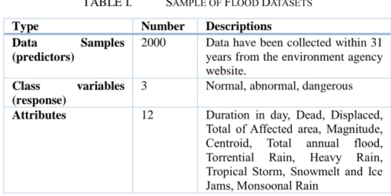
The datasets used in our study is collected from the environment agency website[23]. These datasets are gathered from different cities the around the globe. Each sample involves 12 attributes deemed significant features for predicting the severity as shown in Table I. The main idea behind choosing the severity feature instead of other features is related to the fact that severity feature is considered highly important to the flood
control centre. To deal with a large amount of data, environmental agencies were supported with several flood records. Moreover, the datasets involved 2000 sample points, with 3 target values describing the severity of the flood. The target value was discretised into 3 class labels, target 1 (normal level), target 2 (abnormal one), target 3 (dangerous level). Such a division is important to deliver proper class representation over the datasets sample.
TABLE I. SAMPLE OF FLOOD DATASETS Type Number Descriptions Data Samples
(predictors)
2000 Data have been collected within 31 years from the environment agency website.
Class variables (response)
3 Normal, abnormal, dangerous
Attributes 12 Duration in day, Dead, Displaced, Total of Affected area, Magnitude, Centroid, Total annual flood, Torrential Rain, Heavy Rain, Tropical Storm, Snowmelt and Ice Jams, Monsoonal Rain
B. Exploratory analysis
In order to undertake an exploration of the used data in our experiments, visualisation techniques containing Principal Component Analysis (PCA) has been used as shown in Figure 2. PCA is considered as one of the most popular methods for dimensionality reduction. This type of method performs a linear mapping with lower-dimensional space of the datasets in such way that instance of our data sets representation is maximized. According to our dataset, it is shown that our datasets can be separated. The plots illustrate a number of linearly uncorrelated variables that refer to principal components. The initial component is controlled through their contribution to the maximum instance in the data sets. Then, all other subcomponents are found through the equivalent maximum-variability constraint. The PCA plot (figure. 2) shows that there are possible clusters of values present within the data, a finding that is further elaborated through the tSNE plot as presented in the following section, which demonstrates that the data can be geometrically separated when considering various intervals of dosage level. The statistical tools and computation techniques for our datasets are based on PRTools, a Matlab toolbox used for pattern recognition [24].
Fig. 2. Principal Component Analysis (PCA).
Another kind of, visualisation techniques containing is t-Distributed Stochastic Neighbor Embedding (t-SNE) as demonstrated in figure 3. t-SNE technique is used to represent
dimensionality reduction that suitable to visualise our data sets with high dimensional. t-SNE scales depending on the total number of objects N, it’s appropriate to a limited number of data
sets with few thousand instances. We applied this technique to our data sets up to 2000 instance divided into three classes. The main point of using this method is to show how the 3 classes been demonstrated and the possibility of separating the data sets into three groups.
Fig. 3. T-distributed Stochastic Neighbourhood Embedding (tSNE). Exploratory procedures outcomes expose that some noticeable structure is shown within the flood datasets. The PCA figure demonstrates that there are potential clusters of flood features presented, which shows that the data can be geometrically separated into three classes when observing different intervals of severity level. Fig 3 shows that our flood datasets can be possibly separated and classified.
VI. EXPERIMENTAL PROCEDURE
The experimental setup in this section covers the design of the test environment used in our experiments, the configuration of each model, and the models tested. The performance evaluation techniques used to find out the results of the machine learning algorithms for the flood forecasting datasets.
Holdout technique is applied in our study for the purpose of evaluating how the statistical analysis can generalise to an independent data sets [25]. The total proportion of the flood data sets is divided into training, validation, and testing phases. This method is used to discover an average percentage of the correct classifications or the incorrect classifications. In this context, the training set receives 70%; the validation set receives 10%, while the testing set receives 20%. The flood datasets split into training and testing sets, for the purpose of ensuring that the generalisation error of the classifiers can be evaluated and to demonstrate the capability of classifiers to compute on unseen data.
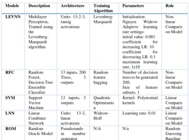
The algorithms are composed of trained classifiers using three kinds of integrated machine learning approaches: RFC, SVM, and LEVNN. The main purpose of selecting these models is to deal with high performance and strong non-linear classifiers. In this context, the linear method model comprises a single layer neural network with a linear transformation function at each class output unit. In order to obtain performance estimates, we calculated the mean of the responses for the proposed algorithms by running each simulation 50 times. Table II describes all models that are used in our experiments. The (LNN) and the (ROM) are applied as baseline classifiers to build
random case performance by the task of random responses for each class.
Our model evaluation framework consists of training and testing diagnostics, supported by five important performance evaluations [10]. It is involved sensitivity (True positive)[26] , specificity (true negative), precision level, the F1 score point (F1), Youden’s J statistic (J1), and accuracy calculated as illustrated in Equations 9 to 13. In addition, the models were characterised using ROC figures and the AUC figures, while the classification capability across operating method was determined. Precision: 𝑇𝑃 =TP+FPTP (9) F1 Score: 𝑇𝑃 =2 ∗ (Precision∗Recall) (Precision+Recall) (10) J1: Sensitivity + 𝑆𝑝𝑒𝑐𝑖𝑓𝑖𝑐𝑖𝑡𝑦 – 1 (11) Accuracy: (TP+FN+TN+FP)(TP+TN) (12)
AUC: 0 <= Area under the ROC Curve <= 1 (13)
TABLE II. THE DESCRIPTIONS OF THE USED MODELS Models Description Architecture Training
Algorithm Parameters Role LEVNN Multilayer Perceptron, Trained using the Levenberg-Marquardt algorithm Units: 13-2-3, tansig activations Levenberg-Marquardt Initialisation: Nguyen Widrow Adaptive learning rate settings: initial value: 0.001 coefficient for increasing LR: 10 coefficient for decreasing LR: 0.1 maximum learning rate: 1e10 Non-linear Comparis on Model RFC Random Forest, Decision Tree Ensemble Classifier 13 inputs, 200 Trees, 3 outputs Random feature bagging Number of decision trees to be generated 200; Size of feature subsets: 1 Non-linear Comparis on Model SVM Support Vector Machine 13 inputs, 3 outputs Quadratic Optimisatio n Kernel: Polynomial kernels Linear Comparis on Model LNN Linear Combiner Network Units: 13-3, linear activations Widrow-Hoff
Learning rate: 0.01 Linear Comparis on Model ROM Random Oracle Model Pseudorando m number generator
N/A N/a Random Guessing Baseline
VII. RESULTS
The results are shown in Tables III and IV for our empirical study, listing the outcomes for the supervised learning techniques, by applying the training and testing of the classifiers, respectively. We also provide very high-performance visualisations through using the receiver operating characteristic curve (ROC) plots (as shown in Figures 4 and 5) and the use of the area under the curve (AUC) plots as illustrated in the bar charts in Figures 6 and 7. The AUC graphs offer a visual comparison in association with the AUC across the classifiers tested.
The outcomes gained from our experiments indicate that the RFC and LEVNN models outperformed all other models. These
models obtain proper fit over the used training sets for all computing points, as illustrated in Table III and the ROC and AUC graphs shown in Figures 4 and 6, respectively. Furthermore, the performance of the LEVNN and RFC classifiers acquired during the training is exposed to provide optimal generalisation to the test data selection, which obtained excellent outcomes in terms of AUCs in average with 3 classes 0.994 for RFC and 0.858 for LEVNN, while obtaining good outcomes during testing process in average 0.877 for LEVNN and 0.907 for RFC. In this context, the strong generalisation of RFC and the LEVNN shows that there occurs rich information within our selected datasets source, presenting a great upper bound on classification in regard with accuracy and performance. We carried out extra experiments using SVM, illustrating that this approach is less capable of classifying our data sets.
The training sets of the LNN classifier model generated accuracy values between 0.296 and 0.744, while the testing sets produced values 0.33 to 0.85 as expected. With this regard, the LNN model was incapable to learn specifically the non-linear components. It yields weak classification outcomes against the other models. Random oracles model was unable to learn the non-linear components and offered modest results, as shown in figure 5 and figure 6 and representing, by contrast, the significance of the outcomes from the other trained models.
TABLE III. PERFORMANCE EVALUATION (TRAINING)
Models Class Precision F1 Score J Score Accuracy AUC
ROM Class 1 0.151 0.172 -0.0274 0.676 0.48 Class 2 0.581 0.3 -0.0167 0.434 0.502 Class 3 0.229 0.222 -0.00431 0.649 0.509 LEVNN Class 1 0.837 0.26 0.148 0.853 0.847 Class 2 0.804 0.838 0.556 0.797 0.876 Class 3 0.679 0.349 0.201 0.796 0.851 RFC Class 1 1 0.375 0.231 0.871 0.997 Class 2 0.981 0.882 0.777 0.871 0.988 Class 3 0.984 0.961 0.934 0.982 0.997 SVM Class 1 0.667 0.0333 0.0154 0.834 0.67 Class 2 0.71 0.781 0.337 0.708 0.782 Class 3 0 0 0 0.768 0.795 LNN Class 1 0.168 0.287 0 0.168 0.634 Class 2 0.6 0.75 0 0.6 0.296 Class 3 0.232 0.377 0 0.232 0.744
TABLE IV. PERFORMANCE EVALUATION (TESTING)
Models Class Precision F1 Score J Score Accuracy AUC
ROM Class 1 0.167 0.194 0.0574 0.749 0.621 Class 2 0.643 0.364 0.0207 0.447 0.546 Class 3 0.24 0.248 -0.00823 0.618 0.565 LEVNN Class 1 0.6 0.194 0.104 0.874 0.829 Class 2 0.772 0.789 0.413 0.731 0.911 Class 3 0.525 0.304 0.151 0.759 0.895 RFC Class 1 1 0.0377 0.0192 0.872 0.864 Class 2 0.897 0.742 0.513 0.726 0.938 Class 3 0.549 0.462 0.291 0.771 0.921 SVM Class 1 0 0 -0.00867 0.862 0.68 Class 2 0.743 0.793 0.364 0.724 0.87 Class 3 1 0.0202 0.0102 0.756 0.89 LNN Class 1 0.131 0.231 0 0.131 0.67 Class 2 0.623 0.768 0 0.623 0.333 Class 3 0.246 0.395 0 0.246 0.85
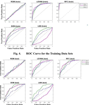
Figures 4 and 5 show the outcomes for each classifier for calculating the training and testing methods of the models. The ROC Curve figures offer a visual comparison across the algorithms tested. In our experiments, we utilised the holdout techniques for distributing training sets and testing sets. In order to train the flood datasets, it is essential to operate two important phases to form the learning schemes. Firstly, we attempt to build the initial structure for each classifier during the training method, to estimate the total error rates as presented in figure 4. Secondly, we evaluate the flood forecasting datasets by applying the testing set in association with predicting the total error rate and accuracy for each classifier as illustrated in figure 5. We compared the performance and error rate through our machine learning classifiers that are used in our experiments over 3 output classes formed into 3 classes: Class 1, class 2, and class3. RFC (test) outperformed among other classifiers and generated the best accuracy as shown in the figures 4 and 5.
Fig. 4. ROC Curve for the Training Data Sets
Fig. 5. ROC Curve per Model for the Testing Data Sets. Class 1 for normal level, class 2 for abnormal level, and class 3 for high risk level.
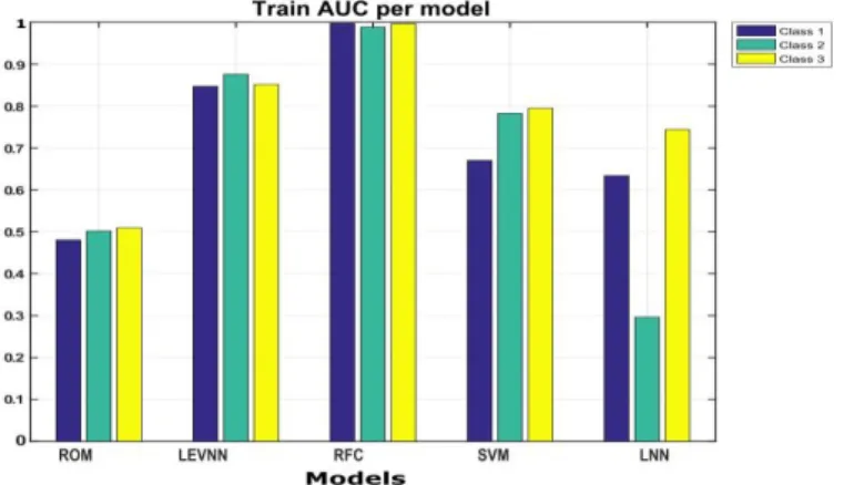
Figures 6 and 7 illustrate the complete outcomes for each class over each classifier within our experiments. AUC demonstrates result each model with three classes. Training set outcomes are illustrated in figure 7, while figure 8 shows the testing set results. In our graphics, the Y-axis demonstrates the AUC that corresponds to each model entries, while the X-axis indicates the classes and models. In our plots, an AUC of one yields an ideal model, whereas an AUC of 0.5 depicts random performance. Each of the bars in the AUC figure plotted is associated with a corresponding curve in both Figures 6 and 7. One main benefit of using AUC plots in our experiments is to emphasise the AUC standards in a great graphical form, in such way that a visual comparison can be drawn.
Fig. 6. Train AUC per Model Using the Training Data Sets Compare to other machine learning approaches, RFC has been proved to obtain a comparable accuracy, despite the fact that being faster. The classification outcomes in terms of accuracy of RFC for class one, class two, and class three for all the variables in the flood datasets are illustrated in Table III and Table IV. RFC also demonstrated crucial overlaps between inputs variables and classes in the training sets. To assess the classification accuracy of the RFC in contrast with other machine learning classifiers, we have estimated the accuracy 0 to 1. The results of the flood datasets are demonstrated in Figures 6 and 7. The three bar graphs for class 1, class 2, and class 3 (training and testing figures) showed RFC outperformed other classifiers as well as yield acceptable accuracy for three classes. Eventually, RFC can be easily employed to multi-class classification, while other models normally deal with binary classification.
Fig 7. Test AUC per Model Using the Testing Data Sets.
The main reason behind RFC outperformed other types of machine learning is due to the type of data and its distribution. We note that each application and datasets present different challenges and diverse relationships among the variables. It is vital to adjust the parameters in each model to build a more accurate predictive model. The data sample method of our data is considered to be much bigger than the total dimensionally of our datasets. According, to deal with the large number of instances in our datasets, Random Forest managed to combine some types of soft non-linear boundaries, especially at the decision surface. In the testing technique, we used an average of 50 trees in order to obtain smooth of separation. Thus, more trees can provide better decision boundaries. We also estimated the probability distribution for the purpose of produce guardians of the split datasets that would provide a better model with high performance and accuracy. The most important point that RFC provided was a good outcome due to the high complexity control and the overfitting that model included.
A. Discussion
In this study, a data science methodology is used that combines 12 features extracted from 2000 records for the prediction of flood severity outcomes. The main reason that our methods powerful is due to the achievement that been made during training and testing phase as shown in table III and IV. The accuracy outcomes of RF showed 0.994 for the training sets, while testing sets produced 0.907, which considerably a great achievement due to the use of nonlinear methods as well as inseparable data sets. Our experiment produced statistical methods that are not affected by outliers as well as to offer methods with better performance with a few departures that control by parametric distributions.
Furthermore, the performance evaluations for data drawn from a number of probability distributions, particularly for distributions that are not standard. RFC is a powerful model for the analysis of flood datasets, as has been proven for this domain to offer strong predication accuracy and performance in comparison with other classifiers. This type of classifiers/algorithm employs the out-of-bag method instead of cross-validation, which enhances the stability of results during training and testing process. A great relationship between input features and target values has been discovered during the development process. The datasets were moderate in size, with 20% of the input features randomly selected for testing and the remaining percentages of 70% and 10% used for training and validation, respectively. In this context, the test set errors were averaged, and the procedure was repeated 50 times.
Generally, RFC preserves the appealing attributes of decision trees, for instance, handling of redundant/irrelevant descriptors, numerous mechanisms of action, the capability to deal both regression and classification, and the ability to handle various kinds of descriptors simultaneously. This model was much faster with respect to the training procedure, in comparison to the ensemble techniques. A key reason that RF produced the highest performance is due to the fact that the
model did not have the issue of over-fit, and most importantly did not require guidance. Some of the variables are mislabelled for our datasets; the algorithm can handle and detect such missing values, in addition to operating effectively on unbalanced and categorical data, which is less viable for other classifiers, such as SVMs. With the integration of accuracy and efficiency in addition to the useful analytical techniques, the RF algorithm constitutes a viable and effective technique for the multi-source classification of flood datasets, where no suitable statistical algorithms are available.
VIII. CONCLUSIONS AND FUTURE WORK
In this study, we have conducted an empirical investigation into the use of different kind of machine learning algorithms for the predictions of flood data in terms of outcome severity. In this study, five types of machine learning model have been investigated, including baseline models, which are used for drawing relative comparisons with other classifiers. The RFC, SVM, LEVNN were used as the main classifiers. While LNN and ROM were applied as the baseline mechanism that utilised for our empirical study. These models are principally used for the purpose of analysing flood forecasting time series obtained from several locations. The target value was discretised into 3 class labels, target 1 (normal level), target 2 (abnormal one)], target 3 (dangerous level). Such a division is important in order to deliver proper class representation over the datasets sample, whereas preserving some level of precision for the severity outcome. However, the results of our experiments illustrated that random forest yields the optimal results in comparison with the benchmarked models. REC yield better outcomes outperform other classifiers during the training set and testing set with 0.994 and 0.904, respectively. In our study, we calculate sensitivity, specificity, precision, the F1 score, J statistic (J1), and accuracy, ROC, and AUC.
Former studies have revealed that Machine learning algorithms show considerable effectiveness for the pre-processing of environmental time-series datasets, as a precursor to the classification of flood data. For future improvement, we consider using other types of machine learning techniques, including the use of global optimisation algorithms, for instance, the genetic algorithm that can expand the scope and scale of this study.
References
[1] M. A. Friedl and C. E. Brodley, "Decision tree classification of land cover from remotely sensed data," Remote Sensing of Environment, vol. 61, no. 3, pp. 399-409, 1997/09/01 1997.
[2] J. J. Moré, "The Levenberg-Marquardt algorithm: implementation and theory," in Numerical analysis: Springer, 1978, pp. 105-116.
[3] M. Khalaf et al., "A Performance Evaluation of Systematic Analysis for Combining Multi-class Models for Sickle Cell Disorder Data Sets," Cham, 2017, pp. 115-121: Springer International Publishing.
[4] C. Cortes and V. Vapnik, "Support-vector networks," Machine learning, vol. 20, no. 3, pp. 273-297, 1995.
[5] L. Breiman, "Random forests," Machine learning, vol. 45, no. 1, pp. 5-32, 2001.
[6] L. Xiaodong, G. Zhongyang, X. Ran, D. Xiaoyan, H. Yizhi, and Y. Shufeng, "Application of Artificial Neural Network in the Typhoon Flood Prediction System-A Case Study in Shanghai, China," in Artificial Intelligence and Computational Intelligence (AICI), 2010 International Conference on, 2010, vol. 1, pp. 191-195: IEEE.
[7] H. Xia and Q. Rao, "Flood Level Prediction on the Basis of the Artificial Neural Network," in 2009 First International Conference on Information Science and Engineering, 2009, pp. 4887-4890: IEEE.
[8] V. Lempitsky, M. Verhoek, J. A. Noble, and A. Blake, "Random forest classification for automatic delineation of myocardium in real-time 3D echocardiography," in International Conference on Functional Imaging and Modeling of the Heart, 2009, pp. 447-456: Springer.
[9] A. S. Al Kafri et al., "Detecting the Disc Herniation in Segmented Lumbar Spine MR Image Using Centroid Distance Function," in Developments in eSystems Engineering (DeSE), 2017 10th International Conference on, 2017, pp. 9-13: IEEE.
[10] M. Khalaf et al., "Machine learning approaches to the application of disease modifying therapy for sickle cell using classification models," Neurocomputing, 2016.
[11] X. Chen, X. Zhu, and D. Zhang, "A discriminant bispectrum feature for surface electromyogram signal classification," Medical engineering & physics, vol. 32, no. 2, pp. 126-135, 2010.
[12] T. K. Ho, "Random decision forests," in Document Analysis and Recognition, 1995., Proceedings of the Third International Conference on, 1995, vol. 1, pp. 278-282: IEEE.
[13] O. Pauly et al., "Fast multiple organ detection and localization in whole-body MR Dixon sequences," Medical Image Computing and Computer-Assisted Intervention–MICCAI 2011, pp. 239-247, 2011.
[14] P. Buhlmann, "Bagging, boosting and ensemble method" in Handbook of Computational Statistics, vol. pp.985–1022., 2012.
[15] Z.-S. Wei, K. Han, J.-Y. Yang, H.-B. Shen, and D.-J. Yu, "Protein–protein interaction sites prediction by ensembling SVM and sample-weighted random forests," Neurocomputing, vol. 193, pp. 201-212, 6/12/ 2016. [16] M. M. Adankon and M. Cheriet, "Model selection for the LS-SVM.
Application to handwriting recognition," Pattern Recognition, vol. 42, no. 12, pp. 3264-3270, 2009/12/01/ 2009.
[17] M. T. Hagan and M. B. Menhaj, "Training feedforward networks with the Marquardt algorithm," IEEE transactions on Neural Networks, vol. 5, no. 6, pp. 989-993, 1994.
[18] O. Fistikoglu and U. Okkan, "Statistical downscaling of monthly precipitation using NCEP/NCAR reanalysis data for Tahtali River Basin in Turkey," Journal of Hydrologic Engineering, vol. 16, no. 2, pp. 157-164, 2010.
[19] R. A. Mitchell and J. J. Westerkamp, "Robust statistical feature based aircraft identification," IEEE Transactions on Aerospace and Electronic Systems, vol. 35, no. 3, pp. 1077-1094, 1999.
[20] C. Pardo, J. J. Rodríguez, J. F. Díez-Pastor, and C. García-Osorio, "Random oracles for regression ensembles," in Ensembles in Machine Learning Applications: Springer, 2011, pp. 181-199.
[21] E. Oja, "Principal components, minor components, and linear neural networks," Neural Networks, vol. 5, no. 6, pp. 927-935, 11// 1992. [22] M. S. Tehrany, B. Pradhan, S. Mansor, and N. Ahmad, "Flood
susceptibility assessment using GIS-based support vector machine model with different kernel types," Catena, vol. 125, pp. 91-101, 2015. [23] public tableau, "Flood Data and resources " [Online]. Available at:
https://public.tableau.com/s/sites/default/files/media/Resources/Flooddat aMasterListrev.xlsx. [Accessed: 10-Oct-2016].
[24] R. P. Duin et al., "PRTools 4-A MATLAB Toolbox for Pattern Recognition. Version 4.1," Delft University of Technology, 2007. [25] M. Khalaf et al., "Recurrent Neural Network Architectures for Analysing
Biomedical Data Sets," in Developments in eSystems Engineering (DeSE), 2017 10th International Conference on, 2017, pp. 232-237: IEEE. [26] A. S. Al Kafri et al., "Lumbar Spine Discs Labeling Using Axial View MRI Based on the Pixels Coordinate and Gray Level Features," in International Conference on Intelligent Computing, 2017, pp. 107-116: Springer.