Overview of machine learning methods in predicting house prices and its application in R

Copyright by Wei-Ta Chen

The Report Committee for Wei-Ta Chen

Certifies that this is the approved version of the following report:

Overview of machine learning methods in predicting house prices and

its application in R

APPROVED BY

SUPERVISING COMMITTEE:

Overview of machine learning methods in predicting house prices and

its application in R

by

Wei-Ta Chen

Report

Presented to the Faculty of the Graduate School of The University of Texas at Austin

in Partial Fulfillment of the Requirements

for the Degree of

Master of Science in Statistics

The University of Texas at Austin

December 2017

Acknowledgements

I would like to thank Dr. Timothy Keitt and Dr. Bindu Viswanathan for their comments and suggestions on my report. With their supports and valuable insights, I am able to publish my report.

v

Abstract

Overview of machine learning methods in predicting house prices and

its application in R

Wei-Ta Chen, M.S. Stat.

The University of Texas at Austin, 2017

Supervisor: Timothy Keitt

This report aims to predict house prices by using several machine learning methods. These methods include ordinary least squares regression, Ridge regression, Lasso regression, and k-nearest neighbor regression. We compare the prediction accuracy by using root mean square error (RMSE) among these models to determine which model performs best in the predictions of house price. The propose of this report is to give an overview of how to perform different models in predicting house prices and its implementation in R.

Table of Contents

List of Tables ... vii

List of Figures ... viii

Chapter 1 Introduction ...1

Chapter 2 Data and methodology ...3

2.1 Data and variable descriptions ...3

2.2 Data exploration and visualization ...4

2.3 Predictor selection ...7

2.3.1 zero-variance predictor detection ...7

2.3.2 Collinearity inspection ...7

2.4 Models...8

2.4.1 Ordinary least squares regression ...8

2.4.2 Ridge regression ...9 2.4.3 Lasso regression ...10 2..4.4 K-nearest neighbor ...10 Chapter 3 Results ...12 Chapter 4 Discussion ...16 Appendix………18 References ...24

List of Tables

Table 1: The description of variables of house data ...3 Table 2: Regression coefficients of OLS model with all predictors ...13 Table 3: Regression coefficients of OLS model without predictors INDUS and

AGE ...14 Table 4: RMSE values on test dataset by using different models ...29

List of Figures

Figure 1: Distribution of MEDV, median house prices……….………5 Figure 2: Boxplot of median house prices ………...….. ………5 Figure 3: Grouped boxplot of median house prices across CHAS……….6 Figure 4: Relationships among median house prices and other predictors……….6 Figure 5: A graphical display of a correlation matrix of the numeric predictors…8 Figure 6: Distribution of residuals……….14 Figure 7: Residual plot………...……15

Chapter 1 Introduction

The importance of collecting and analyzing data reflecting any business activity to achieve competitive advantage is widely recognized. Among all the techniques, one of the modern and main approaches is machine mining. Machine mining is a sub-core of artificial intelligence. It enables computers to learn by itself without being explicitly programmed (Samuel, 1959). The purpose of machine learning is to build algorithms that can receive input data and apply statistical methods to predict output values. The overall goal of the machine mining process is to extract information from a data set and to transform it into an understandable structure for prediction or other further use. Machine learning has already been widely used for many business organizations including banking sector. It can contribute to solving business problems in banking and finance by finding patterns, causalities, and correlations in business information and market prices that are not immediately apparent to managers because the volume data is too large. There are several main tasks apply in business area, such as prediction, classification, detection of relations, explicit modeling, clustering, and deviation detection.

In this report, we used several machine learning methods to predict house prices. These methods include regression and k-nearest neighbor (KNN) models. We also executed model evaluation to determine which model performs better in predicting house prices. The report organizes in the following sequence. First, we introduce our data and its pre-processing before building models. Second, we present the models that are used in

data analysis and how we tune the hyper-parameters. The third part will be the prediction results with testing data using different models. The last section will be discussions and future directions.

Chapter 2 Data and methodology

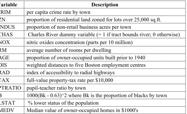
The data used in this report is the famous Boston housing data (Harrison and Rubinfeld, 1978; Belsley et al., 1980). This dataset includes the median value of owner-occupied homes in the Boston area and several other variables that might account for the variation in median house prices. This dataset contains 14 variables and 506 observations. The variable “MEDV” is a numeric response variable, which includes median house prices (Table 1). The rest of variables will be used as predictors to predict the response variable. This dataset will be randomly split into two parts: train (80%) and test (20%) sets. We will build several models using train set and then use these models to predict the median house prices of test set.

Variable Description

CRIM per capita crime rate by town

ZN proportion of residential land zoned for lots over 25,000 sq.ft. INDUS proportion of non-retail business acres per town

CHAS Charles River dummy variable (= 1 if tract bounds river; 0 otherwise) NOX nitric oxides concentration (parts per 10 million)

RM average number of rooms per dwelling

AGE proportion of owner-occupied units built prior to 1940 DIS weighted distances to five Boston employment centres RAD index of accessibility to radial highways

TAX full-value property-tax rate per $10,000 PTRATIO pupil-teacher ratio by town

B 1000(Bk - 0.63)^2 where Bk is the proportion of blacks by town LSTAT % lower status of the population

MEDV Median value of owner-occupied homes in $1000's

2.2 Data exploration and visualization

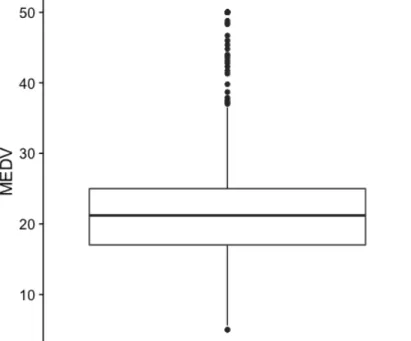
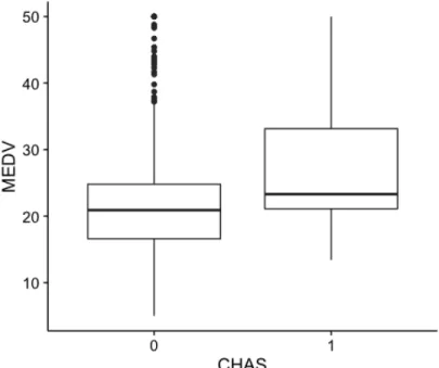
We created a histogram to assess the distribution of the response variable MEDV, median house price (Figure 1). The distribution of MEDV is not normal and displays a right skewed shape. In order to investigate whether there are outliers in this variable, we made a boxplot to detect outliers (Figure 2). There are several potential outliers shown in the boxplot. We need to be aware of these outliers in building models. As there are some houses close to river, we want to know if the proximity to river is a factor influencing the median house prices. The grouped boxplot shows that the median house prices tend to be higher if houses are close to the river (Figure 3). Because most of the variables in this dataset are numeric variables, we made multiple scatter plots to assess the relationship between MEDV and other predictors (Figure 4). As expected, there is a strong positive relationship between the median house prices and the average room number. House prices increases with the number of room (Figure 4B). This is possible due to the fact that more rooms mean a bigger house, which increases the house prices. On the other hand, we observed a negative relationship between median house prices and lower status of population as well as nitric oxides concentration (Figure 4C and 4D). High values of these two predictors accompany with lower median house prices. Regarding to crime rate, it is clear that extreme high crime rate leads to very low median house prices. However, the range of median house price at lower crime is large, suggesting lower crime rate may not be an important factor to determine median house prices (Figure 4A).

Figure 1. Distribution of MEDV, median house prices.

Figure 3. Grouped boxplot of median house prices across CHAS. 1 if tract bounds river; 0 otherwise.

2.3 Predictor selection

There are 13 predictors in the dataset, we perform some procedures to see whether we can remove irrelevant predictors before building models.

2.3.1 Zero-variance predictor detection

If a predictor contains only a constant value, it means every data point has the same value for that predictor. Therefore, this predictor provides no explanation in the data variance of the response variable. Given this point of view, we computed the variance of each numeric feature. The results showed that none of these predictors have zero variance. Therefore, we will not be able to remove any predictors before the development of model.

2.3.2 Collinearity inspection

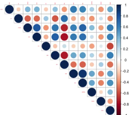
Collinearity is a condition in which some of the predictors are highly correlated with each other. Given the fact that most of these predictors are numeric, we suspected that some of the features might be linearly correlated with each other. To determine whether this is the case in our data, we visualized the correlation matrix of the predictors (Figure 5). If a pair of feature is highly correlated with each other, it will exhibit as a dark blue or dark red dot. The highest correlation coefficient is 0.91 of the pair of TAX and RAD in our data.

Figure 5. A graphical display of a correlation matrix of the numeric predictors in data. Dark blue and dark red dots show highly correlated pairs of features.

2.4 Models

2.4.1 Ordinary least squares regression

Ordinary least squares (OLS) regression is more commonly names as multiple linear regression (at least two predictors) or simple linear regression (one predictor). OLS regression aims to model the relationship between a response variable and one or more predictors by fitting a linear regression (Nimon and Oswald, 2013). Formally, given n observations, the model for OLS regression for p predictors is

yi=b0+b1xi1+b2xi2+…+bpxip+eifor i=1,2, …n, where: yi: response variable

b0-bp: regression coefficients;

e: error term with mean 0 and variance s2

In our data, the response variable is MEDV, median house prices, and the rest of variables are predictors. In order to find the best fit and the regression coefficients (b0-bp)

of the model, OLS regression minimizes the residual sum of squares (RSS) between the actual values in the data and the predicted values by the model. Mathematically speaking, it solves the following equation:

min ||Xb-y||22 ,where b= (b0,…,bp)

Once we have the estimated regression coefficients, we can use these coefficients to predict the response variable.

2.4.2 Ridge regression

Unlike OLS regression, Ridge regression is a regularized model. It is sometimes an issue that OLS regression can be overfitting. An overfitting model means you fit your dataset with a very complicated model and this model can only apply to your current dataset. In other words, we might actually fit random noise instead of reflecting the overall population. Therefore, we want our model to be able to approximately represent the true model for the entire population. That is, our model should not only fit the current sample but also new samples as well. To overcome the overfitting issue, Ridge regression

fits a model by minimizing both the residual sum of squares (RSS) and sum of squares of the regression coefficients:

min ||Xb-y||22 + l ||b||22, where b= (b0,…,bp)

Hence, Ridge regression performs L2 regularization by adding a penalty term equivalent to the squares of the regression coefficients. l is the tuning parameter, which controls balance of fit and the magnitude of regression coefficients (Hoerl and Kennard, 2000).

2.4.3 Lasso regression

Like Ridge regression, Lasso regression is also a regularized model. Instead of using sum of squares of the regression coefficients, it applies sum of absolute value of coefficients to regularize the model to prevent overfitting issue. Mathematically, it solves the following form:

min ||Xb-y||22 + l ||b||1, where b= (b0,…,bp)

That is, Lasso regression performs L1 regularization to by adding l1-norm of the coefficients as a penalty (Tibshirani, 1997). In addition, Lasso regression tends to estimate sparse coefficients, which effectively reduce number of predictors in predicting the response variable.

2.4.4 K-nearest neighbor

algorithm computes the Euclidean distance between the target and the cases of train dataset (Altman, 1992). If K=1, it means the target house price is equal to that of most similar house in the train dataset. If K=k, the target house price is the average of the values of its k-nearest neighbors in the train dataset.

Chapter 3 Results

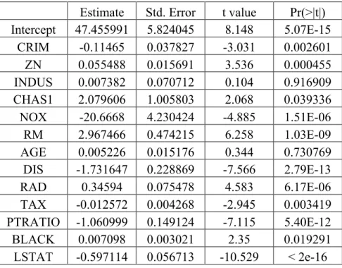
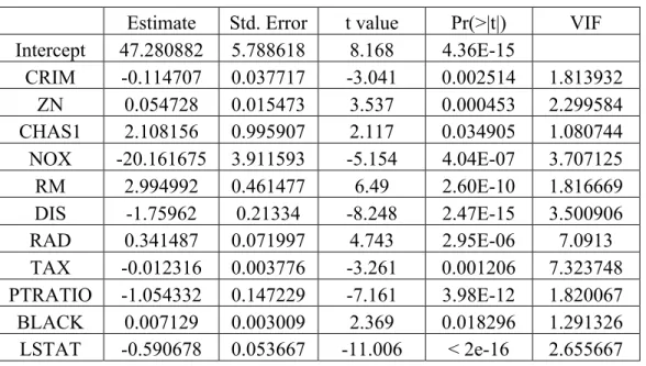
In this report, we aim to predict the response variable of test dataset by using several models built from train dataset. The first model is OLS model. The regression coefficients of OLS model is shown in Table 2. According to this table, we found that two predictors, INDUS and AGE, are not statistically significant. Therefore, we took out the two predictors and re-fit a OLS model again using train dataset (Table 3). As demonstrated in Figure 5, the correlation coefficient between TAX and RAD is 0.91, suggesting the two predictors are highly correlated with each other. To investigate whether multicollinearity occurs in this model, we computed variance inflation factor (VIF). VIF measures the effect of multicollinearity among predictors. The “VIF” column displays the VIF values for each predictor used in the model (Table 3). Both TAX and RAD have high VIF values, which is consistent with the fact that these two predictors also have a high correlation coefficient between them. We can determine whether the VIF values are in an acceptable range based on some guidelines. A common rule of thumb is that if a VIF value is greater than 10, then there is a severe multicollinearity issue in the model. In that case, we need to remove those variables with high VIF values out of the model. Based on the VIF values (Table 3), none of them is greater than 10, indicating multicollinearity did not occur in our train dataset. After fitting the OLS regression model, it is crucial to determine whether the model assumptions are valid before doing inference. If there is a violation of the assumptions, subsequent inferences might be

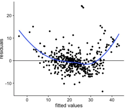
the actual values and the predicted values. The histogram showed an approximate normal to right skewed distribution of the residuals (Figure 6). Based on the residual plot, we found that residuals are not randomly scattered across x axis. Instead, it exhibited a smiley pattern as represented by the blue curve, which suggests independence, constant variance (Homoscedasticity), and linearity assumption do not meet (Figure 7). Next, we used Ridge and Lasso regression to fit our train dataset. By 5-folds cross validation, the tuning parameter lvalue of Ridge and Lasso were found to be 0.7520576 and 0.0257991, respectively. Finally, a k-nearest neighbor (KNN) regression was applied to our train model. The appropriate k value is 4 as determined by 5-folds cross validation.

Estimate Std. Error t value Pr(>|t|) Intercept 47.455991 5.824045 8.148 5.07E-15 CRIM -0.11465 0.037827 -3.031 0.002601 ZN 0.055488 0.015691 3.536 0.000455 INDUS 0.007382 0.070712 0.104 0.916909 CHAS1 2.079606 1.005803 2.068 0.039336 NOX -20.6668 4.230424 -4.885 1.51E-06 RM 2.967466 0.474215 6.258 1.03E-09 AGE 0.005226 0.015176 0.344 0.730769 DIS -1.731647 0.228869 -7.566 2.79E-13 RAD 0.34594 0.075478 4.583 6.17E-06 TAX -0.012572 0.004268 -2.945 0.003419 PTRATIO -1.060999 0.149124 -7.115 5.40E-12 BLACK 0.007098 0.003021 2.35 0.019291 LSTAT -0.597114 0.056713 -10.529 < 2e-16 Table 2. Regression coefficients of OLS model will all predictors.

Estimate Std. Error t value Pr(>|t|) VIF Intercept 47.280882 5.788618 8.168 4.36E-15 CRIM -0.114707 0.037717 -3.041 0.002514 1.813932 ZN 0.054728 0.015473 3.537 0.000453 2.299584 CHAS1 2.108156 0.995907 2.117 0.034905 1.080744 NOX -20.161675 3.911593 -5.154 4.04E-07 3.707125 RM 2.994992 0.461477 6.49 2.60E-10 1.816669 DIS -1.75962 0.21334 -8.248 2.47E-15 3.500906 RAD 0.341487 0.071997 4.743 2.95E-06 7.0913 TAX -0.012316 0.003776 -3.261 0.001206 7.323748 PTRATIO -1.054332 0.147229 -7.161 3.98E-12 1.820067 BLACK 0.007129 0.003009 2.369 0.018296 1.291326 LSTAT -0.590678 0.053667 -11.006 < 2e-16 2.655667

Table 3. Regression coefficients of OLS model without predictors INDUS and AGE. VIF: variance inflation factor.

Chapter 4 Discussion

In this report, we have built several models using the train dataset. In order to compare which model performs well in predicting the median house price, we used root mean square error (RMSE) as an evaluation metric. In regression setting, a commonly used measure to assess the quality of fit is by mean squared error (MSE).

MSE = _"! "_12! observed y − predicted y 2

The square root of MSE is RMSE, which gives us an estimate of how far our predictions will be on average. According to Table 4, the Ridge regression model performs best as its RMSE values is the lowest. In contrast, the predictions from KNN regression are the worst, leading to the highest RMSE value among these models. Therefore, if we want to predict the median house prices of test dataset, we should use Ridge regression model.

When we performed model diagnostics on OLS regression, we found that some of the regression assumptions are not met, such as normality and constant variance assumptions. To deal with these issues, we can perform transformations on our dataset to see whether we can rescue these assumption violations. Once these transformations have been done, and they indeed make regression assumptions meet again. It is possible that the predictions by using OLS regression model will improve and result in a lower RMSE value.

boosting models are also common methods in regression setting. These models are all worth trying in the future to see whether the two models can produce lower RMSE values than that of Ridge regression model.

OLS_1 OLS_2 Ridge Lasso KNN 4.626874 4.6231 4.386957 4.586503 6.147494

Table 4. RMSE values on test dataset by using different models. OLS_1: OLS regression with all predictors. OLS_2: OLS regression without predictors INDUS and AGE. Ridge: Ridge regression. Lasso: Lasso regression.

Appendix

################ install packages

install.packages('MASS') # Boston housing data

install.packages('ggplot2') # Make graphs

install.packages('dplyr') # Manipulate data

install.packages('corrplot') # Make correlation coef plot

install.packages('glmnet') # Lasso and Ridge regression

install.packages('car') # vif function to compute Variance infation factor

(VIF)

install.packages('FNN') # knn.reg: KNN regression

################ load packages

library(ggplot2)

library(dplyr)

library(corrplot)

library(glmnet)

library(car)

library(FNN)

################ rename Boston dataset to house and convert "chas"

variable into factor

data(Boston, package = "MASS") # call out Boston house data

house<- Boston

house$chas <- factor(house$chas)

################ data exploration and visualization

head (house)

str(house)

summary(house) # no missing values

# Find the distrubution of the response variable "medv": right skewed

ggplot(data=house)+geom_histogram(aes(x=medv),

ggplot(data=house, aes(x="",y=medv))+geom_boxplot()+ theme(

axis.title.x=element_blank(),axis.text.x=element_blank(),axis.ticks.x=eleme

nt_blank())+labs(y='MEDV')

# boxplot of chas vs medv: housing prices near river seems to be higher

ggplot(data=house, aes(x=chas, y=medv))+geom_boxplot()+labs(x='CHAS',

y='MEDV')

# check linear relationship using scatter plots

a<-ggplot(data=house, aes(x=crim,y=medv))+geom_point()+labs(x='CRIM',

y='MEDV')

b<-ggplot(data=house, aes(x=rm,y=medv))+geom_point()+labs(x='RM',

y='MEDV')

c<ggplot(data=house, aes(x=lstat,y=medv))+geom_point()+labs(x='LSTAT',

y='MEDV')

d<-ggplot(data=house, aes(x=nox,y=medv))+geom_point()+labs(x='NOX',

y='MEDV')

plot_grid(a, b,c,d, labels=c("A", "B", 'C','D'), ncol = 2, nrow = 2)

################ Data pre-processing: feature selection

# zero-variance predictor detection: none

zero.var <- apply (select (house, -medv), 2, var)

length (which(zero.var ==0))

# inspect collinearity:

corr_feature <- cor (select (house, -c(chas,medv)))

# make a coorplot

################ train and test set split: 80% train and 20% test

set.seed(1)

train_size <- floor (0.8 * nrow (house))

train_row_index <- sample (1:nrow(house), size = train_size, replace =

FALSE)

train <- house[train_row_index, ]

test <- house[-train_row_index, ]

################ OLS model

# OLS model 1: with all predictors

ols_1 <- lm (medv ~.,data=train) # with all predictors

summary(ols_1)

# OLS model 2: without "indus" and "age" predictors

ols_2 <- lm(medv~ ., data=select(train, -c(indus, age)))

summary(ols_2)

vif(ols_2)

# Predictions on test dataset

ols_predicted_1 <- predict(ols_1, newdata = test)

ols_predicted_2 <- predict(ols_2, newdata = test)

# Compute RMSE value on test data

rmse_ols_1 <- sqrt(mean((test$medv-ols_predicted_1)^2)) # 4.626874

rmse_ols_1

rmse_ols_2 <- sqrt(mean((test$medv-ols_predicted_2)^2)) # 4.6231

rmse_ols_2

### Diagnoistics for OLS model

# residual plots

ggplot ()+ geom_point(aes (x=ols_2$fitted.values, y=ols_2$residuals))+

geom_hline(yintercept = 0)+ xlab('fitted values')+ ylab

ggplot ()+geom_histogram(aes (x=ols_2$residuals), bins =35)+

xlab('residuals')+ ylab ('Frequency')

################ Ridge and Lasso regression model

# Prepare feature_matrix and y-vector before using glmnet () since glmnet ()

only works with matrix form

x_train <- model.matrix(medv~.,data=train)

y_train <- train$medv

x_test <- model.matrix(medv~., data=test)

y_test <- test$medv

### select lambda value for Ridge regression

set.seed (10)

ridge_model = cv.glmnet(x = x_train, y = y_train,alpha = 0, nfolds=5) #

alpha= 0 for Ridge

ridge_model$lambda.min

ridge_coef = coef(ridge_model, s = ridge_model$lambda.min)

# Fit Ridge regression with lambda=0.7520576 and predict on test dataset

ridge.fit <- glmnet (x_train, y_train, family="gaussian",

lambda=ridge_model$lambda.min,alpha=0)

# Compute RMSE value on test data

ridge_predicted <- predict(ridge.fit, newx=x_test)

rmse_ridge <- sqrt(mean((test$medv-ridge_predicted)^2))

rmse_ridge

### select lambda value for Lasso regression

set.seed (101)

lasso_model = cv.glmnet(x = x_train, y = y_train, alpha = 1,nfolds=5)

lasso_model$lambda.min # 0.0257991

# Fit Lasso regression with lambda=0.0257991 and predict on test dataset

lasso.fit <- glmnet (x_train, y_train, family="gaussian",

lambda=lasso_model$lambda.min,alpha=1)

# Compute RMSE value on test data

lasso_predicted <- predict(lasso.fit, newx=x_test)

rmse_lasso <- sqrt(mean((test$medv-lasso_predicted)^2))

rmse_lasso

################ KNN regression model

# perform 5-folds CV to determine K (k=4)

set.seed (111)

no_of_folds <- 5

row_index <- sample (1:no_of_folds, size=dim (train)[1], replace = TRUE)

k<- 1:10

mse_matrix <- matrix(NA,nrow=no_of_folds, ncol=10)

name_vec <- rep(NA,10) # create column names

for (i in 1:10)

{

name_vec[i] <- paste('k=',i,sep='')

}

colnames(mse_matrix) <- name_vec # assign column names

for (i in k)

{

for (j in 1:no_of_folds)

{

# train and validation sets

holdout_index = which(row_index== j)

valid_y_array <- y_train[holdout_index]

train_y_array <- y_train[-holdout_index]

# fit models and predict on validation dataset

pred_knn =knn.reg(train = train_X_matrix, test = valid_X_matrix,

y = train_y_array, k = i,algorithm='brute')

# assign mse

mse_matrix[j,i]= mean ((valid_y_array - pred_knn$pred)^2)

}

}

mse_matrix

mean_mse_matrix <- apply(mse_matrix,MARGIN=2,FUN=mean)

which.min(mean_mse_matrix) # k=4, results in lowest mse

# predictions on test data

knn_predicted <- knn.reg(train = x_train, test = x_test, y = y_train, k =

4,algorithm='brute')

# Compute RMSE value on test data

rmse_knn <- sqrt(mean((test$medv-knn_predicted$pred)^2))

rmse_knn

References

Altman, N. S. (1992). "An introduction to kernel and nearest-neighbor nonparametric regression". The American Statistician. 46 (3): 175–185.

Belsley D.A., Kuh, E. and Welsch, R.E. (1980) Regression Diagnostics. Identifying Influential Data and Sources of Collinearity. New York: Wiley.

Harrison, D. and Rubinfeld, D.L. (1978) Hedonic prices and the demand for clean air. J. Environ. Economics and Management 5, 81–102.

Hoerl A.E. and Kennard R.W. (2000) Ridge Regression: Biased Estimation for Nonorthogonal Problems. Technometrics, 42:1, 80-86

Nimon, K. F., and Oswald, F. L. (2013). Understanding the results of multiple linear regression: Beyond standardized regression coefficients. Organizational Research Methods, 16, 650–674.

Samuel, A (1959). Some studies in machine learning using the game of checkers. IBM Journal of Research and Development. 3 (3).

Tibshirani, R (1997). The lasso Method for Variable Selection in the Cox Model. Statistics in Medicine, 16: 385–395.