Bayesian dynamic graphical models for high-dimensional flow forecasting in road traffic networks

(1)

Open Research Online

The Open University’s repository of research publications

and other research outputs

Bayesian dynamic graphical models for

high-dimensional flow forecasting in road traffic

networks

Thesis

How to cite:

Anacleto Junior, Osvaldo (2012). Bayesian dynamic graphical models for high-dimensional flow forecasting in road traffic networks. PhD thesis The Open University.

For guidance on citations see FAQs.

c

2012 The Author Version: Version of Record

Copyright and Moral Rights for the articles on this site are retained by the individual authors and/or other copyright owners. For more information on Open Research Online’s data policy on reuse of materials please consult the policies page.

(2)

THE OPEN UNIVERSITY

Bayesian dynamic graphical models for

high-dimensional flow forecasting in road

traffic networks

by

Osvaldo Anacleto Junior, BSc, MSc

A thesis submitted in fulfilment of the requirements

for the degree of Doctor of Philosophy

I ~ ~:

in the

, ~ ~

~, .,

Department of NIathematics and Statistics

The Open University

November 2012

Dote.

0+

Subnl;~s,cn·.

Iq

oCl

u

ber

20/2-Dot-Q

0t

t\vJard:

5 December

2012

(3)

IMAGING SERVICES NORTH

Boston Spa, Wetherby

West Yorkshire, lS23 7BQ

www.bl.uk

THE FOLLOWING ITEMS HAVE BEEN

EXCLUDED UNDER INSTRUCTION FROM THE

UNIVERSITY

FIGURES

2.1 page

9

(4)

Abstract

Conge~tioll on roads is a crucial problem which affects our lives in many ways. As a consequence, there is a strong effort to improve road networks in order to keep the traffic flowing. Flow forecasting models based on the large amount of traffic data, which are now available, can be a very useful tool to support decisions and actions when managing traffic net.works. Although many forecasting models have been developed to this end, very few of them capture important features of high-dimensional traffic data and, moreover, operating most of these models is a hard task when considering on-line traffic management environments.

Dynamic graphical models can be a suitable choice to address the challenge of fore-casting high-dimensional traffic flows in real-time. These models represent network flows by a graph, which not only is a useful pictorial representation of multivariate t.ime series of traffic flow data, but it also rnsures t.hat model computation is always

~imple, even for very complex road networks. One example of such a model is the

multiregre~::;ion dynamic model (MD~l).

This thesis focuses on the development of two classes of dynamic graphical models to foreca:st traffic flows. Firstly, the linear mult.iregression dynamic model (LMD~l),

which is an l\IDM particular case, is ext.ended to allow important traffic characteris-tics in its structure, such as the heterocedasticity of daily traffic flows, measurement errors due to malfunctions in data collection devices, and the use of extra traffic variables as predictors to forecast flows. Due to its graphical structure, the MDM assumes independence of flows at the entrances of a road network. This thesis therefore introduces a new cla.')s of dynamic graphical models where the correlation across road network entrances is accommodated, resulting in better forecasts when compared to the LMDM.

All the methodology proposed in this thesis is illustrated using data collected at the intersection of three busy motorways near l\lanchester, UK.

(5)

Declaration of Authorship

Some of the work presented in this thesis hClli already been accepted for publication and was collaboratively done as follows.

Part of Chapter 4 and all the developments described in Chapter G have been ac-cepted for publication under the title "Mult.ivariate forecasting of roacl traffic flows in the presence of heterosccdasticity and measurement errors" and will appear in the Joumal of the Royal Statistical Society. Series C (Applied Statistics), volume 2, in 1\1arch, 2013. This paper was co-authored with Catriona. Queen and Casper Albers, with me as the first author. 'While Catriona developed the first theoretical ideas for this paper anel Casper did the preliminary analysis of the data, I developed further the theoretical ideas ba..c;ed on an extensive analysis of available data, also carried out by me. I also did all the practical work to implement the models.

The material in Chapter 6 has been accepted for publication in the Australian and New Zealand 10umal of Statistics under the title "Forecasting multivariate road traffic flows using Bayesian dynamic graphical models, splines and other traffic vari-abIes". This paper \Va..c; also co-authored with Catriona Queen and Casper Albers with me as the first author. Casper proposed the use of traHic variables in flow forecasting models using splines, and also carried out the preliminary data analysis. Based on t.hese developments, I ext.ended t.he data analysis of all the traffic vari-ables considered in this work, proposed a different met.hod to use traffic predictors in forecasting flow models still using splines, and I also extended the use of splines in the context of dynamic graphical models to parsimoniously accommodate high-frequency flow data and to remove previous unrealistic assumptions assumed by the model under study. Catriona supported the theoretical developments for this work and, again, I did all the practical work to implement the models.

A third paper co-authored with Catriona Queen. with me a..s the first author, IS

currently being finished, based on all the research presented in Chapter 7. Here, I

originally proposed all the theory which included the definition of a new dynamic graphical model and the proof of its a..c;sociated results. Catriona played a supporting role in these theoretical developments and gave several suggestions to refine and present them in a clearer manner. All the practical work involved, including data analysis, was also done by me.

(6)

in

61 61 62 64 65 68 70 72 76 77 79 80 80 the LMDM 85 5.1 Introduction... 85

5.2 l\lodelling flow heterosceclasticity 86

5.2.1 Variance laws for

Vi . . . .

87

5.2.2 Discount factors for the observational variance

Vi

90

5.2.3 E x a m p l e . . . 92 5.3 Forecast limits in the LMDl\1 . . . 96 5.3.1 Approximate and simulation-based Ll\IDl\l forecast limits 96 5.3.2 Coverage of Ll\IDl\I foreca..<;t limits . . . 98 5.4 Accommodating measurement errors in the LMDl\l

5.4.1 l\Iea.<mremcnt errors . . . . 5.4.2 Accommodating measurement error 5.4.3 Forecast performance . . . .

99 99 100 101

(8)

Contents v

5.5

Discllssion 102

6 Real-time traffic forecasting: high-frequency flow data and

predic-tor variables with the LMDM 107

6.1 Introduction... 107

6.2 Traffic data aggregation . . . 108

6.3 Modelling the daily flow cycle 109

6.3.1 Cubic splines . . . 110

6.3.2 Cubic splines in the L~ID1\I 111

6.3.3 Example...

6.4 Non-linear traffic predictor variables in the L~lDl\I

6.4.1 Incorporating the predictor variables in the Ll\IDl\l 6.4.2 Model performance . . . . 6.4.3 Root nodes . . . . 6.4.4 Children and grandchildren of the root nodes 6.5 D i s c u s s i o n . . . 7 Extending the MDM: the dynamic chain graph model

7.1 Introduction . . . . 7.2 An MDM restriction . . . . 7.3 The dynamic chain graph model (DCGM)

---7.4 Theoretical results of the DCGl\l . . . 7.5 The linear dynamic chain graph model

(LDCGM) . . . 7.6 Example....

7.6.1 Results. 7.7 Discussion 8 Future work

8.1 Model monitoring and intervention . . . . 8.2 Using downstream flows to forecast upstream flows 8.3 Modelling all weekdays . . . .

114 117

120

122 123

125

127 130 130 130 134 138 147 149

153

155

166 166 167 168 8.4 General chain graph structures for the dynamic chain graph model . . 168 A Moments of LMDM one-step ahead forecast distributions 170 A.l l\lean and variance of conditional one-step ahead forecast distributions 170 A.2 Mean and variance of marginal one-step ahead forecast distributions. 172 A.3 Moments of logical variables . . . 176

(9)

List of Figures

2.1 Aerial photograph of the lvIanchester network (©2012 DigitalGlobe, GeoEye, Infoterra Ltd & Bluesky, The Geolnfonnation Group, I\lap data ©2012 Google) . . . .. 9 2.2 Schematic diagram of the 11anche8te1' network . . . . . 10 2.3 5-min flows (a) and occupancies (b) at site 9200B for May 10th_16th,

2010 . . . , 14 2.4 5-min speeds (a) and head ways (b) at site 9200B for I\lay 10th_16th,

2010. . . .. 15 2.5 Boxplots by .veekdays using 15-min flows for the period 07:00-18:59

(one boxplot for each hour) at site 6013B observed from March to November 2010. . . . . 16 2.6 Scatterplots of 5-min flows at site 9188A at time t venms occupancy,

headway and speed at t -1, in (a) February, (b) .June and (c) October 2010. . . 17

3.1 Fundamental diagram of traffic. 23

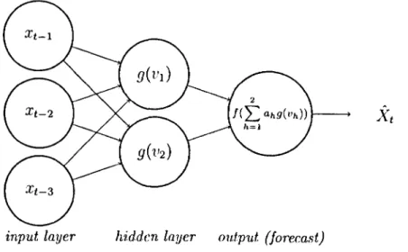
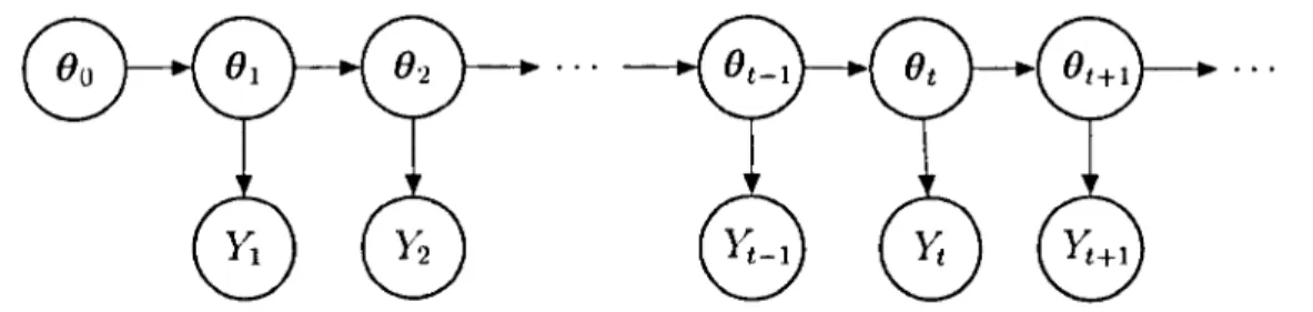
3.2 Neural network example for traffic forecasting 31 3.3 Graphical representation of a stat.e space model (Pet.ris et 0.1., 2009). 0₀

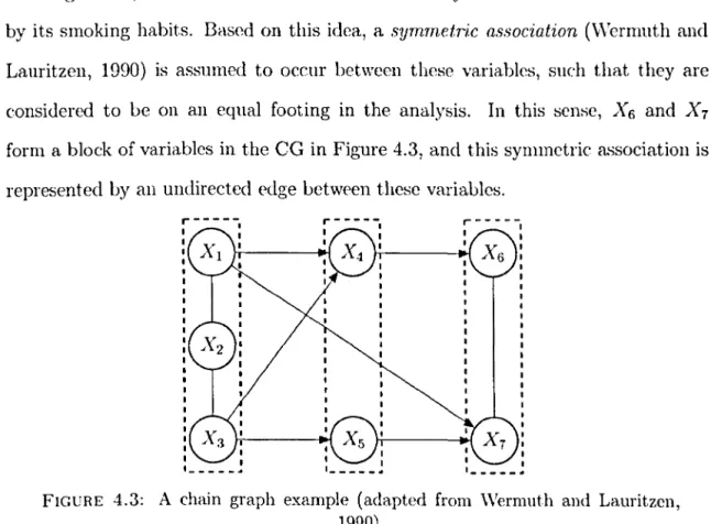
represents the initial information about the state process {Odt~O 35 4.1 A graph. . . 49 4.2 A directed acyclic graph (DAG). . . 51 4.3 A chain graph example (adapted from \Vermuth and Lauritzen, 1990). 53 4.4 A DAG for X =

[Xl!'" ,X4]T . . .

56 4.5 Ancestral graph (a) and moralized ancestral graph (b) to verify whether

AlLBIX,

Y

given the DAG in Figure 4.2 (Cowell

et

aL, 1999). . . .. 59 4.6 A chain graph example (a), together with ancestral graph (b) and

GeoEye, Infoterra Ltd & Bluesky, The Geolnformation Group, Map data ©2012 Google) and (b) schematic diagram: the grey diamonds are the data collection sites, each of which is numbered. The arrows indicate the direction of traffic flow on each part of the network. . .. 73 4.8 DAG for a subset of the London network based on sites 167, 168, 170A

and 170B. . . . . . . . . . 73 vi

(10)

Li!)t of Fig'llTeS vii

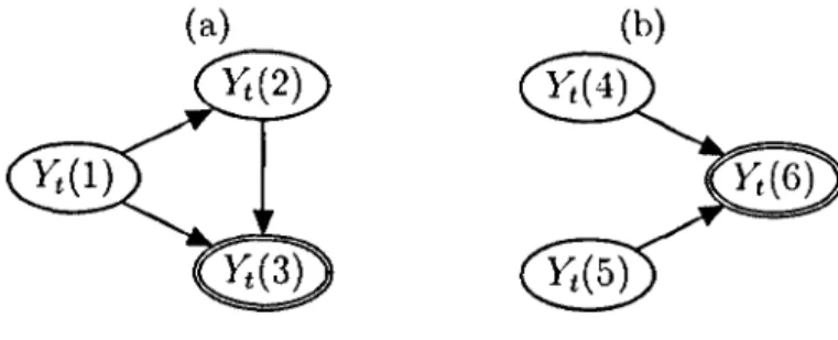
4.9 (a) a fork and (b) a join. In each diagram, the arrows denote the direction of travel and the circles are the sites. . . .. 77 4.10 DAGs representing (a) a fork and (b) a join. The double ovals

repre-sent logical variables. . . .. 79 4.11 DAG for traffic data collection sites in the 11anchester network. . .. 82 4.12 Proportion of traffic flowing from (a) parent 1431A to child 1437 A

and (b) parent 6013B to child G007L during four \Vednesdays in 1\1ay 2010. . . . . 83 4.13 Plot of t.he 15-min flows of parent G013B versus the 15-min flows of

it.s child 6007L for some periods of the day (plot.s on different scales). 84 5.1 Flow mean versus flow variance (log scale, calculated using all

\Vcdnes-days in 2010) at site 920GB: (a) the 48 15-minute periods during 19:00---0G:5D and (b) the 48 15-minute periods during 07:00-18:59 (plots on different scales). . . . 89 5.2 Observed flows on 19 May 2010, a.long with forecast means and forecast

limits bmicd 011 110dels A (red) and B (blue) sites (a) 1431A and (b) 1437A.104 5.3 Observed flows on 19 May 2010, along with forecast limits based on marginal

moments and simulated estimates of the true forecast limits for site 1437 A. 105 5.4 Histogram (a) and q-q plot (b) of errors Yt(1431A) - (Yt{1437 A)

+

Yt(6002A)) in the period 21:00-22:59 during 2010 (excluding 5% of

the extreme errors) . . . 105 5.5 Box plot of the errors Yt(1431A) - (Yi(1437 A)

+ Yt{G002A)) in 2010 .. lOG

6.1 Scatterplots of flows at site 9188A at time

t

versus occupancy,

head-way and speed at t - 1, in (a) February, (b) June and (c) October 2010 . . . 119 6.2 Observed flows at site 9200B on 27 October 2010, along with forecast

means and forecast limits bas('d on LMDl\1s DID and F IF for bivariate series (Yi(9206B), Yt(9200B)). . . . . 128 7.1 5-min flow scatterplots: site 920GB versus site 1431A for some periods

ofthe day: (a) 06:00-06:0-1; (b) 15:00-15:04; (c) 16:25-16:29; (d) 17:25-17:29 (flows observed during Wednesdays from June to November 2010).132 7.2 A chain graph for a subset of data collection sites of the 1Ianchcster

network . . . . . . 133 7.3 Chain graph for the inductive hypothesis (7.11) to (7.14) of the

The-orem 7.2 . . . 143 7.4 Chain graph representing system equations (7.7) and (7.8) of the

DCGM definition . . . 144 7.5 Chain graph representing the observation equations (7.5) and (7.6) of

the DCGM definition. . . . . 145 7.6 Moralized chain graph for the inductive hypothesis (7.11) to (7.14)

(Box A), system equations (Box B) and observation equations (Box C) of the DCG11. . . 158

(11)

List of Fig'uTes

7.7 Moralized chain graph of Figure 7.6, highlighting statemmt (7.15), of the form AlLBIC, from theorem 7.2. C are the violet nodes and A

viii

and B arc orange and brown nodes respectively . . . 159 7.8 1Ioralized chain graph of Figure 7.6, highlighting statement (7.16), of

the form AlLEIC, from theorem 7.2. C are the violet nodes and A

and B are orange and brown nodes respectivciy . . . lGO 7.9 Moralized chain graph of Figure 7.6, highlighting statement (7.17), of

the form AlLEIC, from Theorem 7.2. C are the violet nodes and A

and B arc orange and brown nodes respectively . . . lG 1 7.10 110ralized chain graph of Figure 7.6, highlighting statement (7.18), of

the form AlLBIC, from Theorem 7.2. C arc the violet nodes and A

and B are orange and brown nodes respectively . . . lG2 7.11 Moralized chain graph for the hypothesis of the Corollary 7.3 (Box

A), along with system equations (Box B) and observation equations (Box C) of the DCC lVI at time 1. . . . . . 163 7.12 Observed flows and univariate forpcast limits at site 920GB on 22 Dec

2010 . . . 164 7.13 Observed flows and bivariate forecast. limits

at

root node pair (Yi(l), 1';(2))

(12)

List of Tables

4.1 !\lcdian SE and LPL for LMD!\ls and univariate DL!\ls using 15-min and 5-min flows of the !\Ianchcstcr network . . . . 81 5.1 LPL and MIS for forecasting using !\lodels A D. . 95 5.2 !\IcdianSE for the error model (5.1O) and logical Illodel without an

error term, together with the means and standard deviations of the relative mca.':mrernent errors. . . 102 G.l LPLs for Ll\IDf\Is with different seasonal representations. 116 6.2 LPLs for various models for all root nodes of the !\Ianchcster network. 124 6.3 LPLs for different models for bivariate time series from the

!\lanch-ester network. . . 125 6.4 LPLs for different models for h'ivariate time series from the

!\Iancll-ester network . . .

12G

7.1 LPLs for LMD!\1 and LDCG!\l using diff{'rent Y t subsets 153

(13)

Acknow ledgements

I would firstly like to thank my supervisor, Dr. Catriona Queen. Her invaluable help, guidance, encouragement and several suggestions were crucial to write this thesis and to my development as a statistical researcher. Catriona not only wa.'.; an excellent supervisor, but she also cared a lot about my wellbeing during these past years, for which I am very grateful. I will also always remember her numerous comments on my drafts when trying to clearly and accurately write from now OIl.

During my period as a PhD student, I had the privilege to interact with brilliant researchers from The Open University Statistics Group who are, above all, very kind people. I am very grateful for having this opportunity. I would particularly like to thank Prof. Paul Garthwaite for his suggestions, advice and fruitful discussions regarding the methodology I have developed during my research for this thesis. And also to the Faculty of l\Iathematics and Computing of The Open University for providing me with a PhD scholarship.

Thanks to the Highways Agency for providing the traffic data used in this thesis, anci also to Les Lyman from Matt l\lacDonald for his very important help, patience and time when discussing about analysis of these data.

I strongly believe that one of the best things tha.t happened to my life was to meet people who I can genuinely call friends. Some of them had a profound influence on me while I was doing the research to make this thesis possible, especially when I was facing personal problems which directly affected my academic activities. Here I mention my best friend Andre, who was a constant company during these past three years with his daily e-rnails and frequent Skype calls. Many thanks also to my great friends Ivan and Ana for all the (long) conversations and for being the perfect company in all trips and concerts we have been together.

(14)

Ac;knowledgements Xl

I must also mention some of the people who made my time in Milton Keynes much better: thank you Bethany, Dave, Andy, 1\lariano, Pete and Jay. And I am very grateful to my sister Fabiana., my brother-in-law Aclilson and my nephews Diego and David for making me happy even Leing miles away from me.

Finally, I would like to thank Anna for her constant support, comprehension and patience, particularly when I ended up working most of the time while visiting her. And I extend my deepest gratitude to my mother, whom I will always Le indebted. She has made unmeasurable efforts to provide the best she could give to me and my sister, and only the three of us know how extreme some of the circumstances she had to face were to do so. Her constant encouragem{'nt and comprehension not only helped making this thesis become a reality, but also gave me a strong support to achieve all my goals since my childhood. 1\1ae, mllito obrigado por tueIo!

(15)

Para

minha

mae

(16)

"There will come a time in your life when YO7/, will ask yourself a scries of questions

am I happy with who I am? am I happy with the people around me? am I happy w'ith what

I'm

doing'? am I happy -with the way my life 'is gO'ing'? do I have a life or am I ju::;t living'? do not let these questions restrain or trouble you just point yo'urself in the direction of your d7'eams find your strength in the sound and make your transif'ion"

(17)

Chapter

1 Introduction

This thesis focuses on the problem of developing statistical models for roaJ tmffic flow forecasting. Congestion on roads has become a crucial problem of vital impor-tance during the last decades, since its consequences can affect not ouly daily users of motorways or urban arterials, but also the environment, public health and the economy, for example. As a result, a strong effort has been made by government agencies to maximize ef£ciellcy of road networks to prevent congestion. These de-velopments can be put into practise by defining decision rules or a set of actions to be taken given traffic conditions, and they fonn what is usually called active tmffic

management systems.

One important step for the de\'clopment of these systems in England was the im-plementation of induction loops ill some motorways to collect traffic information, resulting in a huge amount of data which can be updated on a minutc-by-minute bac;is. The analysis of such data is crucial input to improve active traffic manage-ment syst.ems, because it can give insights about current traffic conditions, therefore improving decisions and actions to improve road efficiency.

(18)

Chapter 1. Intr-oduction 2 Since traffic information is generat.rd over time, these data form a time series with possibly very high dimension. Therefore, short-term forecasting models can be useful to describe future traffic conditions. Additionally, since updated traffic conditions a.re obtained as data arrive, an on-line traffic management environment is required. In this context, traffic forecasting models must be also able to provide r-eal-time

forecasts.

This t.hesis will use what are known as dynamic graphical models to forecast traffic flows. ThC'se models represent the flows in the network by a graph. This graph is not only a useful pictorial representation of the network, but it also ensures that model computation is a.lways simple, even for very complex road networks. Although a dynamic graphical model has already heen shown to be extremely promising for short-term foreca.sting in a UK network, t here is still work to be done in order to improve its forecast accuracy when considering real-time traffic data.

1.1 Research question

Traffic data have some characteristics that can be quite challenging to deal with from a statistical modelling perspective. To have a broad view of the traffic network under analysis, data have to be collected from a series of sites, which can generate a high-dimensional time series.

It is also important that a model captures some complex features of road networks. Given a net.work t.opology, traffic flows have a dynamic pattern based on possible driver routes, which defines a dependence structure between the time series: this can heavily affect data analysis and foreca.'lt.s. In addition, events such as adverse traffic conditions or road accidents can cause sudden changes in traffic flows. There may abo be changes in a network due to the development of new motorways or some temporary or permanent road blockages. At the same time, as decisions have

(19)

Chapter 1. Inir'oduci'ion 3

to be taken in real time, especially during busy periods, active traffic management systems require forecasts in an on-line environment.

In view of this, one question that arises is: can a statistical model be capable of generating accurate forecasts given the complexitics from this field, and at the same time be simple enough in ordcr to meet t.he requirements of an active traffic management system? Although it is well known that the model-building process is much more difficult for multivariate time series than univariat.e t.ime series (Chatfield, 2003, \Vest and Harrison, 1997), there are some alternative modelling approaches based on graphical representations of the time series that can address this question.

1.2 Thesis outline

This thesis begins \\'ith a description of an active traHic management system which has been implemented in England, as well as a description of the data used for the development of the proposed models here. These are followed by an analysis of these data, which come from a road intersection in Manchester, UK.

A critical review of the models that have been used so far to forecast. traffic flows is presented in Chapter 3. This chapter also introduces the dynamic linear model, which has a crucial role in the models to be subsequently developed. As will be also discussed in Chapter 3, very few flow forecasting models take into account the multivariate nature of the data.

In

this context, the multiregression dynamic model (MD11), which uses a graph to represent multivariate time series, is presented in Chapter 4. A particular class of 11D1-Is, namely the linear multiregrcssion dynamic model (LMDl\l), has been applied to forecast multivariate flow time series. The U\lDM is also presented in that chapter, followed by a procedure to elicit a graph for the traffic network from which the data are collected.

(20)

Chapter 1. Introduction 4

Both Chapters 5 and 6 show LMDl\l extensions considering traffic dat.a features not previously considered in t.his model, and also taking into account the requirements of active traffic management systems. As will be seen in Chapter 2, it is not reasonable to assume that flow variability is constant over time, as has been assumeu so far when using LMDMs to forecast traffic flows. Chapter 5 therefore shows how to deal with flow heterocedasticity in the U\lDl\1. This chapter also desCTibcs how mea .. <-;urement. errors, due to malfunctions in data collection devices, can be incorporated into this model.

Data currently being collected in English roads are not only flows, but also other traffic variables. There are currently few models which consider t.hese extra traffic variables as predictors in forecasting flow models. Chapter 6 shows hO\v these pre-rlictor variables can be ea.<;ily included into the structure of t.he Ll\lDl\I, resulting in more accurate flow forecasts. Since time series of flows can be built considering different time intervals for uata aggregation, Chapter 6 discusses how different data aggregations show different traffic features. Aduitionally, Chapter 6 shows how the LMDM can accommodate traffic flows aggregated into t.ime intervals suitable for real-time traffic forecasting.

\Vhen using LMDMs to forecast traffic flows, marginal independence is assumed among any time series that represent the entrances of t.he road network under study. However, this assumption may not be reasonable for traffic data. For example, all flows will increase during the build up of traffic in the morning rush hours, and, as another example, auverse weather conditions can affect the road network entrances equally. Motivated by the need of relaxing this restriction, Chapter 7 introduces a new class of dynamic graphical models where the data dependence structure among road network entrances is accommodated, thus resulting in better forecasts when compared to the LMD}'1.

(21)

Chapter 1. Intr'Od'llct'ion 5

Finally, possible future directions to be followed from the proposed statistical devel-opments in this thesis are presented in Chapter 8.

(22)

Chapter 2 The Manchester network

2 .1

Introduction

The traffic data which will be used to develop t.he models described in this thesis are introduced in this chapter, as well as the road intersection where they are col-lected. Time serirs of these traffic dat.a and the relationships between flow and other available traffic variahles are also analysed. We firstly hegin with a description of all active traffic management system currently operating in England.

2.2 The Managed Motorways project

As described in Chapter 1, an active t.raffic management system comprises a set of dech;ion rules or actions to be taken in order to keep the traffic flowing and, especially, to avoid congestion. An example of such system is the Managed Motorways project devc10ped by the Highways Agency, which is responsible for managing and improving road networks in England. An overview of this project can be found in Highways Agency (2012b).

(23)

Chapter 2. The AI an chester network 7

l\lanaged Motorways aims to improve road capacity by controlling the flow using hard shoulders as additional lanes during congestion periods. The usc of hard shoul-ders to reduce levels of congestion hru; been shown to be an useful action in SOllle countries where it was adopted (Sultan ct al., 2008). It is also a cheaper and quicker alternative when compared to widening roads for example. Other actions considered in the l\lanaged Motorways project to improve road efficiency relate to operating mandatory speed limits to controlling flow while traffic is in the network.

These actions depend on alerts \vhich are triggered when certain values of traffic variables are l'xceeded. Particularly, mandatory spct'd limits are triggered when flow readlC's specified (high) values. The data being used in this project are collected by induction loops which were im;talled in some roads in Engla.nd as part of the

Afofo1"way Incident Detection and Automatic Signalling (:MIDAS) system (Gibbens and \Verft, 2005). These inuuction loops are installed at ('ach lalle of a road site, and they collect the following variables on a minutc-by-minute basis:

• Flow: the number of vehicles pa.<,sing over the induction loop per minute; • Occupancy: the percentage of time per minute that vehides arc 'occupying'

the inductive loop;

• Headway: the average time (per minute) between vehicles passing over the inc! uetion loop (in sec);

• (Time mean) speed: the average ratio of the distance between two (conscCll-tive) induction loops in a road segment and the time taken by each vehicle to pru;s over these loops (in kph).

Although these variables are available on a minutc-by-minute basis, data aggregation considering other time intervals may be more suitable, since different traffic features can be observed depending on the aggregation level considered. For the development

(24)

Chapter 2. The Manchester' network 8 of flow forecasting models in this thesis) traffic variables will be averaged into 5-minute and 15-5-minute intervals. Traffic data aggregation will be furthcr discussed in Chapter 6.

The ~Ianaged Motorways project began operating on the M42 motorway in Birm-ingham in 2006, and it is also being implemented in other motorways. See Highways Agency (2012a) for an implementation plan of this project in English road networks.

2.3 The Manchester network

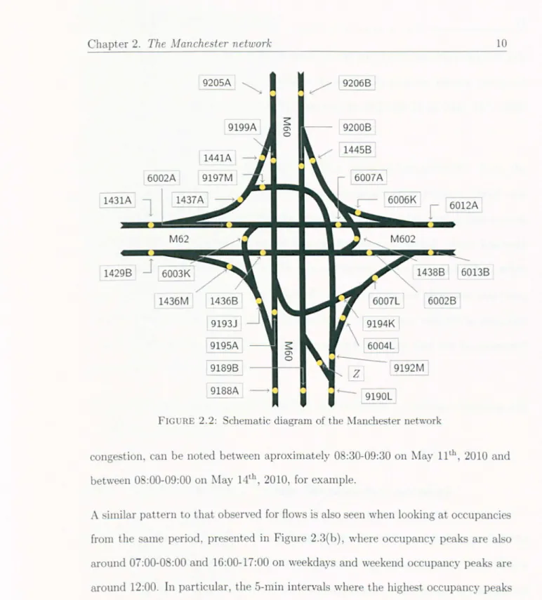
Traffic data collected by inunction loops arc available for the MGO/~IG2/~IG02 in-tersection in Manchester, hereafter called tho Manchester netwoTk) where flow) oc-cupancy, speed and headway information arc collected at 32 sites. Figure 2.1 shows an aerial photograph of the network, and a schematic diagram of the ~Ianchestcr

network reflecting the layout of the data sites is given in Figure 2.2. In this diagram, the alTo\vs show the direction of travel, and the data sites are labelled and indicated by yellow circles. This is one of the networks where Managed Motorways b being implemented (Highways Agency, 2012a).

Given the locations of the data collection sites, it i::; possible to have a description of how traffic flows through the network. One crucial characteristic to be considered when analysing data from this road inter::;ection is that it takes only a few minutes to traverse the Manchester network. This means that vehicles can be counted at a number of different sites during the same time period, depending on the time interval m;ed to aggregate the traffic variables. Information from different parts of the network can therefore be used as potential predictors when developing traffic models for a specific site.

(25)

Chapter 2. The Manchester network

9

2.4 Visualising the Manchester network time

se-.

rles

To visualise some traffic patterns which can be observe,d at the Manchester network, Figures 2.3 and 2.4 show time series plots of flow, occupancy, speed and headway at site 9200B collected between 1Iay 10th and May 16th, 2010. Data were aggregated

into 5-min intervals to plot these series.

Figure 2.3( a) shows a time series plot of 9200B flows. It is clearly seen in this plot that flow patterns during the weekdays are different from flow patterns during weekends: while there are morning and afternoon peak periods around 07:00-08:00 and 16:00-17:00, respectively, on weekdays, a single peak period around 12:00 was observed on both Saturday and Sunday. Some flow outliers, probably caused by

(26)

Chap er 2. The Manchester network 6002A 1431A

1

1429 B

J

,---'.,

9205A 1441A 9197M 9195A: 9189B 9188A ' -9206B 9200B 1445B 6007A

r

6012A 1438B 6013B 6002B

z

9192M I !

FIGURE 2.2: chematic diagram of the Manche ter network

10

conge tion can be noted between aproximately 0 :30-09:30 on May 11th, 2010 and

between 0 :00-09:00 on tvlay 14th, 2010, for example.

A imilar pattern to that observed for flows is also seen when looking at occupancies from the arne period presented in Figure 2.3(b), where occupancy peaks are al 0

around 07:00-0 :00 and 16:00-17:00 on weekday and weekend occupancy peaks are around 12:00. In particular, the 5-min intervals where the highest occupancy peaks

were ob erved during thi week (09:20-09:24 On f\Iay 11th 2010 and 0 :55-0 :59 on

la' 14th 2010) are the same periods where some of the highe t flow peak were

ob erv d in Figure 2.3(a).

Figure 2.4(a) how 5-min peed at site 9200B collected between lay 10th and May

(27)

Chapter 2. The Manchester· network 11 the sense that speeds approximately between 07:00 and 18:00 are lower than speeds observed at other periods during the day. As wit.h flow and occupancy, the most extreme measurements that week were observed at 09:20-09:24 on t-.lay 11th, 2010 and at 08:55-08:59 on t-.Iay 14th, 2010.

The headway plot for this week at site 9200B is given in Figure 2.4(b). Note the high level and also a high headway variability approximatciy between 20:00 and 07:00, which indicates a higher average time between vehicles during this period when compared to headways observed during the daytime period. Since headway is ba<;ed on average times between vehicles per minute, care must be taken ,,,hen analysing this traffic variable during periods where usually low flows are observed: as is quite likely to take more than one minute to observe two vehicles in sequence during low flow periods. Indeed, the ma.ximum headway value that can be measured by loop detectors is 25.4 seconds.

An analysis of the relationship between flow and occnpancy, speed and headway will be presented in Section 2.5.

2.4.1 Flow variability in the Manchester network

Figure 2.5 shows hourly box-plots of 15-min flows for each weekday from 07:00 to 18:59 at site 6013B of the t-.Ianchester network, using data observed from t-.larch to Kovember 2010. These clearly show daily differences in level and \'ariahilitv of v . •

flo,,·s. There is a particularly high flow level observed between 12:00 and 14:59 during Fridays when compared to the same period during other weekdays. On the other hand, there is a lower flow level between 17:00 and 18:59 on Fridays in contrast to the same period during the other weekdays at site 6013ll. It can be an indication that people usually leave work earlier on Fridays.

(28)

Chapter 2. The AI anchester' network 12 Differences in flow variability between weekdays during the same time period are also observed when looking at these boxplot.s. As an example. t.he flow variability observed on Fridays is lower than the flow variaLility oll1Iondays during 18:00-18:59 at site 6013B. Additionally, flow can also vary depcnding on the time of the day, as flow variability observed during 07:00-08:59 is higher than the flow variability observed between 09:00-13:59, for instance.

In Chapter 5, the variability of flows within days will be accommodated in a multi-variate flow forecasting model.

2.5 Relationships between flows and other traffic

variables

As will be discllssed in Chapter 6, there is currently few flO\\' forecasting models which consider extra traffic information in the form of predictor variables. Hence, it is important to analyse the relationship between flows amI extra available variables to have some insights into how to include them as predictors when modelling flows. The first row of Figure 2.6 shows scatterplots of flow at time t versus occupancy at previous time t - 1 at site 9188A for February, June and October 2010. The plots indicate an increasing relationship between flow and occupancy until the latter reaches some value around 20, which is usually defined by traffic managers as the road capacity and varies from sitc to site. For occupancy values higher than this road capacity, the relationship then turns to be decreasing, which can lead to congestion. This relationship is similar to what is called the fundamental diagram of traffic (Ashton, 1966, Kiihne, 2008), which will be discussed ill Subsection 3.2.2 of Chapter 3.

(29)

Chapter 2. The AI anchester network 13 Scat.terplots of flow at time t versus headway at previous time t - 1 at the same site for the same three months are shown in the second row of Figure 2.6. These plots confirm an intuitive relationship in the sense that the flow decreases as the average time between cars increases.

The last. row of Figure 2.6 shows scatterplots of flow at. time t versus speed at pre-vious time t - 1, again at site !H88A for the same three months. l\lost flow values are concentrated at speed values between 80 kph and 100 kph, with an apparently decreasing relationship in this region. There also seems to be an increasing rela-tionship between flo\\! at t and speed at t - 1 for low speed values, although with a slight ly higher level of variability: it is likely that many of these points are from situations where congestion occurred.

Plots of flow at. t versus the other traffic v~U'iahles at t -1 look broadly comparable at the other sites. Based in t.hese observed relat.ionships, it. will be described in Chapter 6 how these extra traffic variables ran be included as predict.ors in a multivariate flow forecasting model.

(30)

::! o c: ;0 l':l I'-' W Ci1 I

2.

::l :D o :;: en ~ '-"' il> ;:l 0-o n n C 1'-''0 Oil> ... ;:l O n . iii' en ,-.. cY ~ o o ~ o o C") o o N o o ~ o \\l 0 .".. ~ .".. CD ( 0 I'-' 0 o C") o tJj 0' .., ?'"

i

... o N 9. 0 =-I ... 0") p. o

5-min flows at site 92008 of the Manchester network from 10/05/2010 to 16/05/2010

8 12 16 20 8 12 16 20 0 8 12 16 20 0 8 12 16 20 a -4 8 12 16 20 a 8 12 16 20 a 8 12 16 20

10/05/2010 11/05/2010 1210512010 13/0512010 1410512010 15105/2010 1610512010

(Mon) (Tue) (Wed) (Thu) (Fri) (Sat) (Sun)

5-min occupancies at site 92008 of the Manchester network from 10/05/2010 to 16/05/2010

8 12 16 10/05/2010 (Mon) 20 4 8 12 16 20 0 1110512010 (Tue) 4 8 12 16 20 0 8 12 16 20 0 1210512010 131051201 0 (Wed) (Thu) 4 8 12 16 14/0512010 (Fri) 20 0 8 12 16 20 0 15/0512010 (Sat) 4 8 12 16 20 16/0512010 (Sun) .---.... Q:> ' - " .---.... cY ' - " 0 ::> Q:> '0 M-et> _..., tv ~ Cb

I~

\:l ;:,-Cb en N-Cb "4 ;;:l Cb N-t: 0 "4 ?;-... ~

(31)

~ (;) c ;0 C'l tv ~ ClI I S 5' UJ '0 <t> <t> 0-UJ """ _Il' ' - " ~ 0- ::r-<t> tv P' 0 0 -... :;: O il' , '< UJ """ 0-' - " P' .,... g!, .,... <t>

'"

tv 0 0 tJj 0' .... ?' _... ~ ... 0

..

::r I ... O'J ;: o N ...--o o o CX) o to o ~ o N I..() ...--o I..() o

5-min speeds at site 92008 of the Manchester network from 10/05/2010 to 16/05/2010

8 12 16 20 0 10105/2010 (Mon) 8 12 16 20 11/05/2010 (Tue) 4 8 12 16 20 0 1210512010 (Wed) 8 12 16 20 0 8 12 16 20 0 8 12 16 20 0 8 12 16 20 13/05/2010 14/05/2010 15/05/2010 16/0512010 (Thu) (Fri) (Sat) (Sun)

5-min headways (in sec) at site 92008 of the Manchester network from 10/05/2010 to 16/05/2010

4 8 12 16 20 10105/2010 (Moo) 8 12 16 20 11/0512010 (Tue) 8 12 16 20 0 12105/2010 (Wed) 8 12 16 20 0 8 12 16 20 0 13/05/2010 14/05/2010 (Thu) (Fri) 8 12 16 20 0 1510512010 (Sat) 8 12 16 20 16/05/2010 (Sun) /"""0. P' ' - " /"""0. 0-' - " 0 ::r-P' "d _.,... <t> "'1 tV ~ ('1)

I~

(") ;:,-('1) en ... ('1) "i ;:j ('1) ... EO 0 "i ?;-... c.n

(32)

60136: 01:00-01:59 60136: 08:00-08:59 60136: 09'00-09:59 60136: 10:00-10:59

9

0''Tl

~

.g;

;;0

§ § § § ~ o-C:: _~ - - - _~ o trl ~ S< S< 8 .

.f3

1-':> --:- ~ --:- ~ ~ as ~ ~ . ~ as '" ""-3 [ 0 §

.

~~n=H=;:3

11

§

_

SSE?

§

~

§

~

~ trl . .-.:....-.:.... : .-.:....-.:....-.:... ~ ~ . . . E$3,.,;;. . . . --~~~ ... S;: 0 8 8 8~~~~~ g~ ~~~' t:> ~ >< " " " " ;:l n~ n ::ro 8 8 8 8 ;;::,-:::::r-Cri N N N N ("t)

o Man Tue Wed Thu ~n Mon Tue Wed Thu ~n Mon Tue Wed Thu ~n Mon Tue Wed Thu F'n Cr.>

C g day of the week day of Ihe week day of the week day of the week

r;:-0 ~ ~ :2 60136: 11:00-11:59 60136: 12:00-12:59 60136: 13:00-13:59 6013B: 14:00-14:59 ;:l ~rn ~ ~ ~ ~ ~ Ul;:O;- - - - ~

g-~~ § § § § ~ m~ - - ~ O U l ~c S< 8 S< 8 ~: ~ . w~. as <Xl as . '" --:- . r - l r'--l _ trl !:l ~ --:- ~ _ ~ ~ ~ ~ - _ Q c::::::l c:::::I . o ()q § ~ ~ ~ ...-L--. . . . . § _ . . . ~-;.. ~ § "'-~=r= '-':'" g .-.:....-.:....-.:... 0" ~ _~~_ . ~ ~ ~ ~ ~ ~ ~ ~ ~ 9"' 0 - - - ' - ...t... ~...- 0 0

..., 2

a 0 8 0 < v 'It v ..,. ro . o.!:l 8 8 8 8 "'""'"':I::D N N N N

(3 52 Mon Tue Wed Thu F'n Mon Tue w'ed Thu F'ri Mon Tue Wed Thu F'ri Mon Tue Wed Thu F'ri S ;;3 day of the week day of the week day of the week day of the week ~ 0' 60136: 15:00-15:59 6013B' 16'00-16:59 6013B: 11:00-11'59 60136: 18:00-18:59 P>"" 8 8 8 8 ri;' ~ ~ ~ ~ ::r ro § § ~ . --:- --:- § . ~ § o'g - ~ . . . ~ - ~SBS

--:-

-

- ~EJS

--:-

-j

.

~ Z::1· ~ ~

B

E;:3 ~ . . ~ J... J... .-.:... ~ 8 J... .-.:... : .-.:... . . .

8 .

: .

~

8.

~:.-.:... ~ ~ ~

'"

.-.:....-.:...

'"

BElo

--:-S~

§ g g g . . .

~

-0" .. ro 0 ..., 0 8 8 8 8J _~ l'V~ v 'It ,. ...,. o 00 ~ .. 8 8 8 8 ~~ N N N N • • , .

Man Tue Wed Thu . F'ri Mon Tue Wed Thu F'n Mon Tue Wed Thu Fri Mon Tue Wed Thu

day of the week day of the week day of the week I ~

(33)

Chapter 2. The ManchesteT netwoTl.; ₁₇ '"<. t." ₀ 0 0 l/') co ~

..

0 '<t ₀ <X> ... .!. <0 .!. Ql iii _.!. .c ₀ iii 0 _M >->- 0 iii U 0 "0 C ~ CD 0 III

i

a. "0 :>

..

~ ₀ 8 IV _en :I: N 0 '<t 0 '<t 0 0 N N 0

009 om: oo~ 0 009 00£ oo~ 0 009 00£ oo~ 0

MOl;! MOl;! MOl;!

, c-o 0 ., 0 l/') <i' 0 '<t ₀ <X> .!. <0 .!. Ql _iii iii .!. c: 0 1ii ::;) M >->- 0 ..., g III _CD _"0 III _~

.,

e

a. "0 8. G III CD _en 0 u :I: N 0 '<t 0 "<t 0 C> 0 ₀ N N 0 009 00£ oo~ 0 009 00£ oo~ 0 009 00£ oo~ 0

MOl;! MOl;! MOl;!

0 ₀ lO 0 co 0 '<t 0 <X> ~ .'.. CD .!.

"'

0 iii _1ii _.'.. ::;) M >-iO .0 0 '" 0 c ~ CD _al '" III U. a. "0

.,

:J III _a. ~ 0 _IV en 0 0 :I: N 0 "<t 0 '<t 0 0 N N 0 009 00£ oo~ 0 009 00£ oo~ 0 009 00£ oo~ 0 MO(;! _MOl;! MOl;!

FIGUR 2.6: _catte_r_p_l_{ots o}_f₅_-min_O_o_,,_'s_{at s}_i_te₉₁ _A_{at t}_im_e_t_v_e_r_s_u_s₀ _c_up_a_n_cy

(34)

Chapter 3 Literature review: previous and

current approaches to traffic

modelling

3.1 Introduction

Traffic modelling has attracted the attention of many researchers since the second half of the twentieth century, where there has been a great development of highway networks and an increa::ie in the number of vehicles in most countries. This attention resulted in an extensive literature with several traffic modelling approaches. The variety of backgrounds of researchers who have been working in this field is also quite noticeable, a.', \Yell a.s the wide variety of journals where their papers have been published. This makes an exhaustive study of all the possible approaches to traffic modelling a very difficult task.

Deterministic views of traffic dynamics use mathematical modelling, and such de-velopments have provided important concepts about traffic behaviour. The first

(35)

Chapter 3. Litrmt'llre review 19 statistical applications in the field were based on ARIl\fA models, which are es-tablished forecasting tools for time series. Multivariate ARIl\lA versions, namely VARl\lA models~ have been recently considered for traffic forecasting. Due to their flexibility and the variety of commercial software available, neural network models have also been extensively applied in traffic modelling. Additionally~ applications of state space models have been considered in this field, since their structure permits a sequential estimation of parameters for forecasting traffic flows. These are the approaches to be discussed in the next sections.

Some reviews covering the broad extent of mathematical traffic flow models can be found in Bellomo et al. (2002), Hoogendoorn and Bovy (2001) and Gartuer et

al. (2001). Van Arel1l et aZ. (1997), Vlahogianni

et

al. (200-1) and Karlaftis and Vlahogiallni (2011) review neural network techniques, statistical approaches and also some hybrid alternatives for short-term traffic forecasting.

3.2 Mathematical modelling of traffic flows

The initial approaclws to model traffic had a mathematical basis, where determin-istic relationships between traffic parameters in space and time were considered. l\lathematical traffic flm\" models can be classified according to the level of detail defined to describe traffic behaviour. They are then basically divided into micro-scopic and macroscopic models. There is also a third type of models where analogies between flow of vehicles in a road and the flow of molecules in a gas are considered (Ashton, 1966).

(36)

Chapter 3. Literature review 20

3.2.1 Microscopic models

1\Iicroscopic models are used to have a description of the dynamics of individual drivers, taking into account the influence of surrounding vehicles (Bellomo et al.,

2002). Their main idea is to establish a mechanism describing a.<;pects of the inter-action between vchicles through mathematical formulations.

1\10st early attempts to develop microscopic models form what are called car-following models, which arc ba.<;ed on descriptions of how one vehicle fo11O\vs another (Chandler et oL, 1958). Given a sequence of vehicles following each other, the basic principle uscd in these models considers the response, which is the act of accelerating or brak-ing related to the followbrak-ing vehicle, as a product of what are known as scnsitivity and stimulus. Stimulus is defined as the spel'd difference between the leader and the follower in the sequence. Sensitivity can be viewed as a measure of interaction between vehicles, usually defined to be inversely proportional to the' space between them (Edie, 1961, Herman and Potts, 1961). l\1athematical expressions of these quantities can be found in Chandler et al. (1958) and Gazis et al. (1961). Some alternative principles and approaches to define interaction betwecn individual vehi-cles and other types of microscopic models can be found in Hoogendoorn and Bovy

(2001).

Car-following principles have been heavily applied in the development of simulation tools to have a computer-based view of traffic behaviour, resulting in seyeral micro-scopic simulation models. Ba'>ed on some initial conditions about driver behaviour and vehicle characteristics, simulation methods are used to determine how the traffic system evolves over time, given possible decisions each driver can make. A review of microscopic simulation models was made in the S1\IARTEST project (Algers et 0,1.,

1997), where the main objective was to develop this class of models to solve specific traffic management problems.

(37)

Chapter 3. Litemture review 21 Although these models can be quite useful to understand traffic behaviour, they demand a high level of detail about traffic data. Alternatively, traffic information on an aggregated level can be u::ied to generate microscopic data (Hoogencloorn and Bovy, 2001), and some effort has been made to build suitable datascts for the development of such models (\Vilson, 2010). However, given the structure of microscopic models, it can be quite difficult to update them in an on-line traffic environment, since the generation of real-time forecasts as new data arrive possibly requires a high number of simulations.

3.2.2 Macroscopic models

. Different from car-following approaches, macroscopic models can be used to give a description of traffic on an aggregated level, not taking into account explicit rela-tionships between different vehicles. Their basic principle is that driver behaviour depends on traffic characteristics that can be defined in terms of aggregated variables mca .. 'mrcd at a road of interest.

The first study concerning traffic flow behaviour adopted a macroscopic approach and was made by Grecnshields (1935). In this work, the focus was on determining the road conditions in which congestion or slow traffic are likely to occur. Traffic measurements and relationships developed by Greenshields had a significant impact in the field during the following decades.

The model developed in this first study focused on the relationship between three traffic variables:

• flow (q): number of vehicles per unit time;

• density or concentration (k): number of vehicles per unit distance; • mean speed (u): distance per unit of time.

(38)

Chapter 3. Litemt'llT'e T'eview 22 The relation

q = u x k. (3.1)

can be defined among these variables. Greenshields used a 16 mm camera to measure these quantities in a road by taking pictures at regular time intervals (sec Green-shields, 1934, for details). l\Iotivated by his measurements, he realized that a linear relationship of the form

u = a -

13k,

(3.2)

for some a and (3, could be a..<;sumcd between speed and concentration.

Taking into account that concentration reflects the level of interaction between ve-hicles in a road, it can be noted that, a..<; this variable (k) tends to zero, the speed

(u) tends to reach its maximum. In equation (3.2), a is usually called the free

speed, which is considered as the maximum speed a driver can reach if there are 110

interactions between vehicles in a road. On the other hand, the ratio

a/

(3 can be considered as the maximum concentration as speed tends to zero. Replacing (3.2) in (3.1) we have,

(3.3)

which represents a quadratic relationship between flow and concentration (as shown in Figure 3.1) and, as mentioned in Section 2.5 of Chapter 2, i::; called the funda-mental diagram of traffic.

\Vith this simple model and its empirical validation (Greenshields, 1935), it is pos-sible to describe some intuitive traffic flow characteristics. For example, it is rea-sonable to assume that flow must be zero when concent.ration is zero, and also concentration reaches its ma..ximum when traffic jams occur. It can be also thought that flow increa.<;es up to a given value and, after reaching it, interactions between "ehicles are so high that flow tends to decrease, leading to a traffic jam. This value

(39)

Chapter 3. Liter·at'llre r·eview

c:

-road capacity km<l oL---~~--~._---concentration (k)

FIGURE 3.1: Fundamental diagram of traffic.

23

is called the road capacity and it is of great interest for traffic engineers in order to design new roads or to monitor traffic.

Alt.hough the equation proposed by Greenshiclds was widely accepted as the proper shape of the flow-concentrat.ion curve, some aut.hors pointed out limitations of this model (see, for example, Ashton, 1966). Gartner

et

al. (2001) also noted that Greenshielcls' measurements were made during a holiday in a single lane road, where the lcvel of interaction betwcen vehicles is lower than levels observed in multi-lane freeways. There are indeed studies which propose different relationship descriptions of flow-concentration, speed-concrntration and flow-speed. There has also been some effort to describe these three variables simultaneollsly (Gilchrist, 1988, Gilchrist and Hall, 1989). Equations describing these relationships are usually called

traffic stream

models.

Additionally, there are some models (Edie, 1961, Greenberg, 1959) which consider discontinuites in t.he flow-concentration relationship, with different regimes during non congestion times (t.raffic flow values smaller than road capacity) and congestion times (t.raffic flows bigger than road capacity). It can reflect a limitation found in Ashton (1966) regarding Greenshields' model, where it was observed that the flow-concentration relationship canllot be considered to be the same for all values of k, since a driver probably only takes account of the vehicle ahead when driving in low concentrations, and several factors begin to influence him as concentration

(40)

Chapter 3. Litemture review 24 increa..<;es.

3.2.2.1 Hydrodynamic approaches to traffic modelling

l\lacroscopic traffic models can be also developed by considering analogies between vehicular and fluid flows. These analogies motivate the formulation of partial dif-fcrential equations which, together with their solutions, can dcscribe the dynamics of macroscopic traffic characteristics (such as flow, concentration and speed) thus giving a picture of how traffic behaves over time. These models are usually called

continuum flow models (Gartner et al., 2001).

The key idea behind continuum flow models is what is called the principle of flow conseT1lation, which can be stated as follows. Suppose a road section with two data collection sites, namely 5(1) and 5(2), such that they are separated by a very small distance bo.r, therc arc not any intersections or junctions betwcen them and the direction of traffic is from 5(1) to 5(2). The principle of flow conservation st.ates that the increase in the flow at the downstream site 5(2) during a very small time

bot must be equal to the decrease of vehicles (concentration) in the section of the road between sites S(l) and 5(2). This principle can be mathematically described (3.4) where Dq/D.r represents the increase in flow at 5(2) and -ok/at represents the decrease of vehicles in the section of the road between sites S(l) and 5(2) (for details, sec Ashton, 1966). If entrances or exits in a road section arc considered, equation (3.4) can be written as (Gartner et al., 2001),

Dq Dk

(41)

Chapter 3. Literature 1'eview 25 where 9(:r, t) is the generation (or dissipation rate) of vehicles per time per unit length. Equation (3.5) is usually called the conservation equation.

Different solutions exist to the conservation equation, either by usmg aJditional equations or by considering the description of other macroscopic variables. Particu-larly, Payne (1971) considered a partial differential equat.ion descri bing the dynamic behaviour of speed, and this idea was also used in Helbing (1996).

Lighthill and \Vhit.ham (19.55) were the first to propose a solution to (3.5), con-sidering a system with the conservation equation, the relationship given in (3.1)

and assuming speed a.s a function of concentration (such as (3.2)). A similar solu-tion was derived by Richards (1956), with thi::; approach being usually called L\VR (Light hill, \Vhitham and Richard::;) models. A::; this class of models docs not have a unique solution, some generalized solutions were proposed by Lcut:lbach (1988), and a description of numerical alternativcs can be found in Gartner

ct ai.

(2001). Stephanopoulos and 1Iichalopoulos (1979, 1981) describe some implementations of L\VR models.

Since loop detectors in road networks collect traffic macroscopic data (as seen in Chaptcr 2), continuum flow models are presumably suitable for traffic foreca.sting. However, these data are used in continuum flow models to estimate additional equa-tions to solve the conservation equation (3.5). As the resulting system of equaequa-tions may not have closed-form solutions, it can then be infeasible to use them on a real-time basis. Some other limitations of macroscopic models can be found in Pa-pageorgioll (1998).

(42)

Chapter 3. Liter'ature r'eview 26

3.3 ARIMA models in traffic forecasting

After the seminal work of Yule (1927), which introduced the notion of defining a time series as a realization of a stochastic process, there were several developments to describe dynamic systems using time series models with a random component, rather than considering strictly deterministic mathematical models only. In this context, given a sequence of random variables

{xtl

t~l, which represents a time series of interest, a general class of models consists of describing the random variable at time

t

a'l a sum of a linear combination representing a function of previous values of the

sequence, together with a linear combination of random variables with zero mean and constant variance, snch that

p q

Xt =

L

Q.jXt -i

+

L

(3jZt-j (3.6)

i=l )=0

where Zt-j, j = 0, ... ,q, are random variables with null mean and constant variance, and

/30

= 1.

The first sum in (3.6) represents the systematic term of what is called a autoregress'ive process of order p, denoted by AR(p). The idea is that the observed value of the random variable at time t depends on previous observed values of the sequence, and it has the same structure of the systematic term of the classic linear model, despite the fact that the systematic term in a autoregressive process contains realizations of the same random variable defined as the response (hence the name autoregressive). The second sum represents a moving average process of order q, denoted by ~1A(q),

and it can be interpreted as being composed of the error term of the model at time

t,

represcnted by Zt, as wc also have in the classical linear model, plus the error terms related to differences between predicted and observed values at previous times, represented by Zt-j, i = 0, ... , q.

(43)

Chapter 3. Litemture review 27 The parameters to be estimated in this model from an observed time series are Qi and

Pj'

i = 1, ... , p, j

=

1, ... , q. Using this terminology, the model described in (3.6) is usually called an autoregress'ive mov'ing average process of order (p, q), or simply ARI\lA(p, q).

The key assumption in the estimation of ARMA models is that some statistical properties of the sequence of random variables, which represents the time series under study, must remain the same over time. Particularly, this means that {Xth~l must satisfy two conditions:

i.

E[Xtl

and Var[Xtl are constant for every t

2:

o.

ii. Cov[Xt,

Xt-sl

depends only on the difference t-8, that is, the covariance between

two clements of the sequence of random variables depends only on the lag between them, and not on time

t.

A time series which satisfies conditions (i) and (ii) above is said to be weakly sta-tionary or just stationary.

Transformations are usually applied to make a sequence of observed time series sta-tioIlary, with the differencing technique being the most common one. A differenced time series is defined as the sequence {vdXth~d+ll ,,,here each VdXt corresponds to the difference Xt - Xt -d , with t

2:

d

+

1. \Vhen (3.6) is applied to a differenced time series, we can write

p q

Vd X t

=

l'Vt

=

L

Qi

n't-i

+

L

Pj

Zt-j (3.7)

i=l j=O

and then we have what is called the autoregressive integrated moving average process of order (p, d, q) or simply ARIMA(p, d, q), where d is related to the lag applied in differencing the original time series. The term integrated refers to the fact that forecasts based on the transformed series must be summed (or "integrated") to