Online Learning:
Theory, Algorithms, and Applications
Thesis submitted for the degree of “Doctor of Philosophy”
by
Shai Shalev-Shwartz
Submitted to the Senate of the Hebrew University
July 2007
This work was carried out under the supervision of
Prof. Yoram Singer
To Moriah and Meitav
הֹנְק
הָמְכָח
הַמ
;ץוּרָחֵמ בוֹטּ
.ףֶסָכִּמ רָחְבִנ ,הָניִבּ תוֹנְקוּ
[ז"ט ,ז"ט ילשמ]
“How much better to get wisdom than gold, to choose understanding rather than silver”
[Proverbs 16:16]
Acknowledgments
First, I would like to express my deep gratitude to my advisor, Yoram Singer. Yoram has had a profound influence on my research. He exposed me to the fascinating world of online learning. I have learned a variety of research skills from Yoram including scientific writing, basic analysis tools, and (hopefully) good taste in choosing problems. Besides being a good teacher, Yoram is also a great friend.
I would also like to thank the other members of my research committee: Jeff Rosenschein, Mike Werman, and Mira Balaban.
I collaborated and wrote papers with great people. Thank you Yonatan Amit, Koby Crammer, Ofer Dekel, Michael Fink, Joseph Keshet, Andrew Ng, Sivan Sabato, and Nati Srebro.
I am fortunate to have been a member of the machine learning lab at the Hebrew university. I would like to thank former and current members of the lab for being a supportive community and for your friendship. Thank you Ran, Gal E., Gal C., Amir G., Amir N., Adi, Noam, Koby, Lavi, Michael, Eyal, Yossi, Naama, Yonatan R., Yonatan A., Tal, Ofer, Menahem, Tamir, Chen, Talya, Efrat, Kobi, Yoseph, Ariel, Tommy, Naomi, Moran, Matan, Yevgeni, Ohad, and forgive me if I forgot someone.
Being a Ph.D. student at the computer science department at the Hebrew university has been a fan-tastic experience. I had the pleasure of attending fascinating courses and getting advice from brilliant re-searchers such as Tali Tishby, Nati Linial, Irit Dinur, Nir Friedman, Yair Weiss, Daphna Weinshall, and Amnon Shashua. I would also like to thank the administrative staff of the computer science department for totally easing the burden of bureaucracy. Special thanks goes to Esther Singer for making a great effort to correct my English at very short notice.
Yair Censor from Haifa University guided me through the world of optimization and row action methods. He has been a major influence on this thesis.
During the summer of 2006 I interned at IBM research labs. I would like to thank Shai Fine, Michal Rosen-Zvi, Sivan Sabato, Hani Neuvirth, Elad Yom-Tov, and the rest of the great people at the machine learning and verification group.
Last but not least, I would like to thank my family and in particular my wife Moria for her support, patience, and love all along the way.
Abstract
Online learning is the process of answering a sequence of questions given knowledge of the correct answers to previous questions and possibly additional available information. Answering questions in an intelligent fashion and being able to make rational decisions as a result is a basic feature of everyday life. Will it rain today (so should I take an umbrella)? Should I fight the wild animal that is after me, or should I run away? Should I open an attachment in an email message or is it a virus? The study of online learning algorithms is thus an important domain in machine learning, and one that has interesting theoretical properties and practical applications.
This dissertation describes a novel framework for the design and analysis of online learning algorithms. We show that various online learning algorithms can all be derived as special cases of our algorithmic framework. This unified view explains the properties of existing algorithms and also enables us to derive several new interesting algorithms.
Online learning is performed in a sequence of consecutive rounds, where at each round the learner is given a question and is required to provide an answer to this question. After predicting an answer, the correct answer is revealed and the learner suffers a loss if there is a discrepancy between his answer and the correct one.
The algorithmic framework for online learning we propose in this dissertation stems from a connection that we make between the notions ofregretin online learning andweak dualityin convex optimization. Regret bounds are the common thread in the analysis of online learning algorithms. A regret bound measures the performance of an online algorithm relative to the performance of a competing prediction mechanism, called a competing hypothesis. The competing hypothesis can be chosen in hindsight from a class of hypotheses, after observing the entire sequence of question-answer pairs. Over the years, competitive analysis techniques have been refined and extended to numerous prediction problems by employing complex and varied notions of progress toward a good competing hypothesis.
We propose a new perspective on regret bounds which is based on the notion of duality in convex optimization. Regret bounds are universal in the sense that they hold for any possible fixed hypothesis in a given hypothesis class. We therefore cast the universal bound as a lower bound
for an optimization problem, in which we search for the optimal competing hypothesis. While the optimal competing hypothesis can only be found in hindsight, after observing the entire sequence of question-answer pairs, this viewpoint relates regret bounds to lower bounds of minimization problems.
The notion of duality, commonly used in convex optimization theory, plays an important role in obtaining lower bounds for the minimal value of a minimization problem. By generalizing the notion of Fenchel duality, we are able to derive a dual optimization problem, which can be opti-mized incrementally, as the online learning progresses. The main idea behind our derivation is the connection between regret bounds and Fenchel duality. This connection leads to a reduction from the process of online learning to the task of incrementally ascending the dual objective function.
In order to derive explicit quantitative regret bounds we make use of the weak duality prop-erty, which tells us that the dual objective lower bounds the primal objective. The analysis of our algorithmic framework uses the increase in the dual for assessing the progress of the algorithm. This contrasts most if not all previous works that have analyzed online algorithms by measuring the progress of the algorithm based on the correlation or distance between the online hypotheses and a competing hypothesis.
We illustrate the power of our framework by deriving various learning algorithms. Our frame-work yields the tightest known bounds for several known online learning algorithms. Despite the generality of our framework, the resulting analysis is more distilled than earlier analyses. The frame-work also serves as a vehicle for deriving various new algorithms. First, we obtain new algorithms for classic prediction problems by utilizing different techniques for ascending the dual objective. We further propose efficient optimization procedures for performing the resulting updates of the online hypotheses. Second, we derive novel algorithms for complex prediction problems, such as ranking and structured output prediction.
The generality of our approach enables us to use it in the batch learning model as well. In particular, we underscore a primal-dual perspective on boosting algorithms, which enables us to analyze boosting algorithms based on the framework. We also describe and analyze several generic online-to-batch conversion schemes.
The proposed framework can be applied in an immense number of possible real-world applica-tions. We demonstrate a successful application of the framework in two different domains. First, we address the problem of online email categorization, which serves as an example of a natural online prediction task. Second, we tackle the problem of speech-to-text and music-to-score alignment. The alignment problem is an example of a complex prediction task in the batch learning model.
Contents
Abstract vi
1 Introduction 1
1.1 Online Learning . . . 1
1.2 Taxonomy of Online Learning Algorithms . . . 2
1.3 Main Contributions . . . 4
1.4 Outline . . . 6
1.5 Notation . . . 7
1.6 Bibliographic Notes . . . 9
I Theory 11 2 Online Convex Programming 12 2.1 Casting Online Learning as Online Convex Programming . . . 12
2.2 Regret . . . 14
2.3 Non-convex loss functions and relative mistake bounds . . . 15
2.4 Bibliographic notes . . . 17
3 Low Regret and Duality 18 3.1 Online Convex Programming by Incremental Dual Ascend . . . 18
3.2 Generalized Fenchel Duality . . . 19
3.3 A Low Regret Algorithmic Framework for Online Convex Programming . . . 20
3.4 Analysis . . . 22
3.5 Automatically tuning the complexity tradeoff parameter . . . 26
3.6 Tightness of regret bounds . . . 31
3.7 Bibliographic notes . . . 32
4 Logarithmic Regret for Strongly Convex Functions 34
4.1 Generalized Strong Convexity . . . 34
4.2 Algorithmic Framework . . . 35
4.3 Analysis . . . 37
4.4 Bibliographic Notes . . . 39
II Algorithms 40 5 Derived Algorithms 41 5.1 Quasi-additive Online Classification Algorithms . . . 41
5.2 Deriving new online updates based on aggressive dual ascending procedures . . . . 49
5.3 Complex Prediction Problems . . . 55
5.4 Bibliographic Notes . . . 62
6 Boosting 64 6.1 A Primal-Dual Perspective of Boosting. . . 64
6.2 AdaBoost . . . 67
6.3 Bibliographic Notes . . . 69
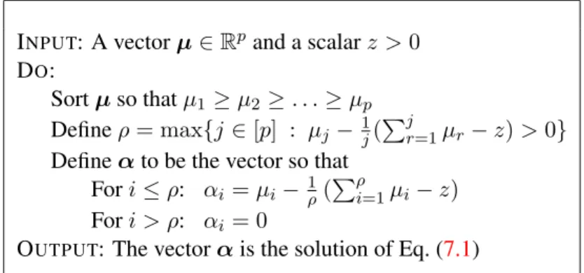
7 Efficient Implementation 70 7.1 Projections onto`1Balls and onto the Probabilistic Simplex . . . 70
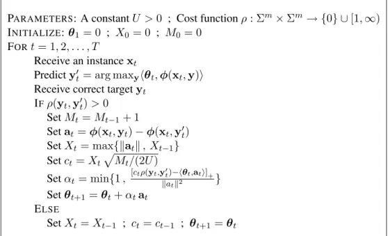
7.2 Aggressive Updates for the Hinge-loss . . . 76
7.3 Aggressive Updates for Label Ranking . . . 78
7.4 Aggressive Updates for the Max-of-Hinge loss function . . . 87
7.5 Bibliographic Notes . . . 89
III Applications 90 8 Online Email Categorization 91 8.1 Label Ranking. . . 91
8.2 Hypothesis class for label ranking . . . 92
8.3 Algorithms . . . 92
8.4 Experiments . . . 94
8.5 Bibliographic Notes . . . 95
9 Speech-to-text and Music-to-score Alignment 96
9.1 The Alignment Problem . . . 96
9.2 Discriminative Supervised Learning . . . 98
9.3 Hypothesis Class and a Learning Algorithm for Alignment . . . 98
9.4 Efficient evaluation of the alignment function . . . 100
9.5 Speech-to-phoneme alignment . . . 101 9.6 Music-to-score alignment . . . 104 9.7 Bibliographic Notes . . . 107 10 Discussion 108 Bibliography 110 Appendices 120 A Convex Analysis 120 A.1 Convex sets and functions . . . 120
A.2 Gradients, Subgradients, and Differential Sets . . . 120
A.3 Fenchel Conjugate . . . 121
A.4 Strongly Convex Functions . . . 124
A.5 Technical lemmas . . . 132
B Using Online Convex Programming for PAC learning 140 B.1 Brief Overview of PAC Learning . . . 140
B.2 Mistake bounds and VC dimension . . . 142
B.3 Online-to-Batch Conversions . . . 142
B.4 Bibliographic Notes . . . 151
Chapter 1
Introduction
This introduction presents an overview of the online learning model and the contributions of this dissertation. The main concepts introduced here are covered in depth and more rigorously in later chapters.
1.1
Online Learning
Online learning takes place in a sequence of consecutive rounds. On each round, the learner is given a question and is required to provide an answer to this question. For example, a learner might receive an encoding of an email message and the question is whether the email is spam or not. To answer the question, the learner uses a prediction mechanism, termed a hypothesis, which is a mapping from the set of questions to the set of admissible answers. After predicting an answer, the learner gets the correct answer to the question. The quality of the learner’s answer is assessed by a loss function that measures the discrepancy between the predicted answer and the correct one. The learner’s ultimate goal is to minimize the cumulative loss suffered along its run. To achieve this goal, the learner may update the hypothesis after each round so as to be more accurate in later rounds.
As mentioned earlier, the performance of an online learning algorithm is measured by the cu-mulative loss suffered by the learning along his run on a sequence of question-answer pairs. We also use the termexampleto denote a question-answer pair. The learner tries to deduce information from previous examples so as to improve its predictions on present and future questions. Clearly, learning is hopeless if there is no correlation between past and present examples. Classic statistical theory of sequential prediction therefore enforces strong assumptions on the statistical properties of the input sequence (for example, it must form a stationary stochastic process).
CHAPTER 1. INTRODUCTION 2
In most of this dissertation we make no statistical assumptions regarding the origin of the se-quence of examples. We allow the sese-quence to be deterministic, stochastic, or even adversarially adaptive to our own behavior (as in the case of spam email filtering). Naturally, an adversary can make the cumulative loss of our online learning algorithm arbitrarily large. For example, the adver-sary can ask the same question on each online round, wait for the learner’s answer, and provide the opposite answer as the correct answer. To overcome this deficiency, we restate the learner’s goal based on the notion ofregret. To help understand this notion, note that the learner’s prediction on each round is based on a hypothesis. The hypothesis is chosen from a predefined class of hypothe-ses. In this class, we define the optimal fixed hypothesis to be the hypothesis that minimizes the cumulative loss over the entire sequence of examples. The learner’s regret is the difference between his cumulative loss and the cumulative loss of the optimal fixed hypothesis. This is termed ’regret’ since it measures how ’sorry’ the learner is, in retrospect, not to have followed the predictions of the optimal hypothesis. In the example above, where the adversary makes the learner’s cumulative loss arbitrarily large, any competing fixed hypothesis would also suffer a large cumulative loss. Thus, the learner’s regret in this case would not be large.
This dissertation presents an algorithmic framework for online learning that guarantees low regret. Specifically, we derive several bounds on the regret of the proposed online algorithms. The regret bounds we derive depend on certain properties of the loss functions, the hypothesis class, and the number of rounds we run the online algorithm.
1.2
Taxonomy of Online Learning Algorithms
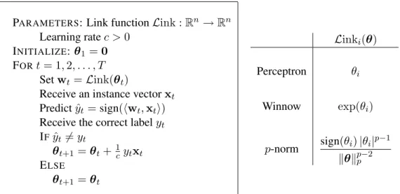
Before delving into the description of our algorithmic framework for online learning, we would like to highlight connections to and put our work in context of some of the more recent work on online learning. For a more comprehensive overview of relevant publications see Section1.6 below and the references in the papers cited there. Due to the centrality of the online learning setting, quite a few methods have been devised and analyzed in a diversity of research areas. Here, we focus on the machine learning and pattern recognition field. In this context, the Perceptron algorithm [1,95,91] is perhaps the first and simplest online learning algorithm and it will serve as our starting point.
The Perceptron is designed for answering yes/no questions. The algorithm assumes that ques-tions are encoded as vectors in some vector space. We also use the term “instances” to denote the input vectors and the term “labels” to denote the answers. The class of hypotheses used by the Per-ceptron for predicting answers is the class of linear separators in the vector space. Therefore, each hypothesis can be described using a vector, often called a weight vector. For example, if the vector space is the two dimensional Euclidean space (the plane), then instances are points in the plane and hypotheses are lines. The weight vector is perpendicular to the line. The Perceptron answers
CHAPTER 1. INTRODUCTION 3
yes no yes
no
Figure 1.1: An illustration of linear separators in the plane (R2). The solid black line separates the
plane into two regions. The circled point represents an input question. Since it falls into the “yes” region, the predicted answer will be “yes”. The arrow designates a weight vector that represents the hypothesis.
“yes” if a point falls on one side of the line and otherwise it answers “no”. See Figure1.2for an illustration.
The Perceptron updates its weight vector in an additive form, by adding (or subtracting) the input instance to the weight vector. In particular, if the predicted answer is negative whereas the true answer is positive then the Perceptron adds the instance vector to the weight vector. If the prediction is positive but the true answer is negative then the instance vector is subtracted from the weight vector. Finally, if the predicted answer is correct then the same weight vector is used in the subsequent round.
Over the years, numerous online learning algorithms have been suggested. The different ap-proaches can be roughly divided into the following categories.
1.2.1 Update Type
Littlestone, Warmuth, Kivinen, and colleagues proposed online algorithms in which the weight vector is updated in amultiplicativeway. Examples of algorithms that employ multiplicative updates are the Weighed Majority [85], Winnow [82], and Exponentiated Gradient (EG) algorithms [75]. Multiplicative updates are more efficient then additive updates when the instances contain many noisy elements. Later on, Gentile and Littlestone [59] proposed the family ofp-norm algorithms that interpolates between additive and multiplicative updates.
This flurry of online learning algorithms sparked unified analyses of seemingly different online algorithms. Most notable is the work of Grove, Littlestone, and Schuurmans [62] on a quasi-additive
CHAPTER 1. INTRODUCTION 4
family of algorithms, which includes both the Perceptron [95] and the Winnow [82] algorithms as special cases. A similar unified view for regression was derived by Kivinen and Warmuth [75,76].
1.2.2 Problem Type
The Perceptron algorithm was originally designed for answering yes/no questions. In real-world applications we are often interested in more complex answers. For example, in multiclass catego-rization tasks, the learner needs to choose the correct answer out ofkpossible answers.
Simple adaptations of the Perceptron for multiclass categorization tasks date back to Kessler’s construction [44]. Crammer and Singer [31] proposed more sophisticated variants of the Perceptron for multiclass categorization. The usage of online learning for more complex prediction problems has been further addressed by several authors. Some notable examples are multidimensional regres-sion [76], discriminative training of Hidden Markov Models [23], and ranking problems [28,29].
1.2.3 Aggressiveness Level
The update procedure used by the Perceptron is extremely simple and is rather conservative. First, no update is made if the predicted answer is correct. Second, all instances are added (subtracted) from the weight vector with a unit weight. Finally, only the most recent example is used for updating the weight vector. Older examples are ignored.
Krauth [78] proposed aggressive variants of the Perceptron in which updates are also performed if the Perceptron’s answer is correct but the input instance lies too close to the decision boundary. The idea of trying to push instances away from the decision boundary is central to the Support Vector Machines literature [117,33,100]. In addition, various authors [68,57,80,74,103,31,28] suggested using more sophisticated learning rates, i.e., adding instances to the weight vector with different weights.
Finally, early works in game theory derive strategies for playing repeated games in which all past examples are used for updating the hypothesis. The most notable is follow-the-leader ap-proaches [63].
1.3
Main Contributions
In this dissertation we introduce a general framework for the design and analysis of online learning algorithms. Our framework includes various online learning algorithms as special cases and yields the tightest known bounds for these algorithms. This unified view explains the properties of existing algorithms. Moreover, it also serves as a vehicle for deriving and analyzing new interesting online learning algorithms.
CHAPTER 1. INTRODUCTION 5
Our framework emerges from a new view on regret bounds, which are the common thread in the analysis of online learning algorithms. As mentioned in Section1.1, a regret bound measures the performance of an online algorithm relative to the performance of a competing hypothesis. The competing hypothesis can be chosen in retrospect from a class of hypotheses, after observing the entire sequence of examples.
We propose an alternative view of regret bounds that is based on the notion of duality in con-vex optimization. Regret bounds are universal in the sense that they hold for any possible fixed hypothesis in a given hypothesis class. We therefore cast the universal bound as a lower bound for an optimization problem. Specifically, the cumulative loss of the online learner should be bounded above by the minimum value of an optimization problem in which we jointly minimize the cu-mulative loss and a “complexity” measure of a competing hypothesis. Note that the optimization problem can only be solved in hindsight after observing the entire sequence of examples. Neverthe-less, this viewpoint implies that the cumulative loss of the online learner forms a lower bound for a minimization problem.
The notion of duality, commonly used in convex optimization theory, plays an important role in obtaining lower bounds for the minimal value of a minimization problem (see for example [89]). By generalizing the notion of Fenchel duality, we are able to derive a dual optimization problem, which can be optimized incrementally as the online learning progresses. In order to derive explicit quantitative regret bounds we make immediate use of the weak duality property, which tells us that the dual objective lower bounds the primal objective. We therefore reduce the process of online learning to the task of incrementally increasing the dual objective function. The amount by which the dual increases serves as a new and natural notion of progress. By doing so we are able to associate the cumulative loss of the competing hypothesis (as reflected by the primal objective value) and the cumulative loss of the online algorithm, using the increase in the dual.
Different online learning algorithms can be derived from our general framework by varying three components: the complexity function, the type of the loss function, and the dual ascending procedure. These three components correspond to the three categories described in the previous section; namely, to the update type, the problem type, and the aggressiveness level. We now briefly describe this correspondence.
First, recall that in the primal problem we jointly minimize the cumulative loss and the com-plexity of a competing hypothesis. It turns out that different comcom-plexity functions yield different types of updates. For example, using the squared Euclidean norm as a complexity function results in additive updates whereas by using the relative entropy we obtain multiplicative updates. Sec-ond, our framework can be used in conjunction with a large family of loss functions. Therefore, by constructing a loss function that fits a particular prediction problem, we immediately obtain online algorithms for solving this prediction problem. Last, the regret bounds we derive for the framework
CHAPTER 1. INTRODUCTION 6
hold as long as we have a sufficient increment in the dual objective. By monitoring the increase in the dual we are able to control the aggressiveness level of the resulting online learning algorithm.
To make this dissertation coherent and due to the lack of space, some of my research work was omitted from this thesis. For example, I have also worked on boosting and online algorithms for regression problems with smooth loss functions [38,40], online learning of pseudo-metrics [109], online learning of prediction suffix trees [39], online learning with various notions of margin [103], online learning with simultaneous projections [4], online learning with kernels on a budget [41], and stochastic optimization using online learning techniques [110].
1.4
Outline
The dissertation is divided into three main parts, titled Theory, Algorithms, andApplications. In each part, there are several chapters. The last section of each of the chapters includes a detailed review of previous work relevant to the specific contents described in the chapter.
1.4.1 Part I: Theory
In the theory part, we derive and analyze our algorithmic framework in its most general form. We start in Chapter2with a formal description of online learning and regret analysis. We then describe a more abstract framework called online convex programming and cast online learning as a special case of online convex programming. As its name indicates, online convex programming relies on convexity assumptions. We describe a common construction used when the natural loss function for an online learning task is not convex.
Next, in Chapter 3we derive our algorithmic framework based on the relation between regret bounds and duality. Our presentation assumes some previous knowledge about convex analysis, which can be found in ChapterAin the appendix. We provide a general analysis for all algorithms that can be derived from the framework. To simplify the representation, we start the chapter with a description of a basic algorithmic framework that depends on a parameter. This parameter reflects the trade-off between the cumulative loss of the competing hypothesis and its complexity. We later suggest methods for automatically tuning this parameter. We conclude the chapter by discussing the tightness of our bounds.
The regret bounds we derive in Chapter 3for our general algorithmic framework grow as the sqrt root of the number of online rounds. While this dependence is tight in the general case, it can be improved by imposing additional assumptions. In Chapter4we derive online learning algorithms with logarithmic regret, assuming that the loss functions are strongly convex.
CHAPTER 1. INTRODUCTION 7
PAC learning framework. For completeness, in Chapter Bgiven in the appendix, we discuss the applicability of our algorithmic framework to the PAC learning model. We start this chapter with a short introduction to the PAC learning model. Next, we discuss the relative difficulty of online learning and PAC learning. Finally, we propose general conversion schemes from online learning to the PAC setting.
1.4.2 Part II: Algorithms
The second part is devoted to more specific algorithms and implementation details. We start in Chapter5by deriving specific algorithms from our general algorithmic framework. In particular, we demonstrate that by varying the three components of the general framework we can design algorithms with different update types, different aggressiveness levels, and for different problem types.
Next, in Chapter6we show the applicability of our analysis for deriving boosting algorithms. While boosting algorithms do not fall under the online learning model, our general analysis fits naturally to general primal-dual incremental methods. As we discuss, the process of boosting can be viewed as a primal-dual game between a weak learner and a booster.
Finally, in Chapter 7 we discuss the computational aspects of the different update schemes. Depending on the loss function and update scheme at hand, we derive procedures for performing the update with increasing computational complexity.
1.4.3 Part III: Applications
In the last part of the dissertation we demonstrate the applicability of our algorithms to real world problems. We start with the problem of online email categorization, which is a natural online learning task. Next, we discuss the problem of alignment. The alignment problem is an example of a complex prediction task. We study the alignment problem in the PAC learning model and use our algorithmic framework for online learning along with the conversion schemes described in the appendix (ChapterB) to construct an efficient algorithm for alignment.
1.5
Notation
We denote scalars with lower case letters (e.g. xandλ), and vectors with bold face letters (e.g. x
andλ). Theith element of a vectorxis denoted byxi. Since online learning is performed in a
sequence of rounds, we denote byxtthetth vector in a sequence of vectorsx1,x2, . . . ,xT. Theith
CHAPTER 1. INTRODUCTION 8
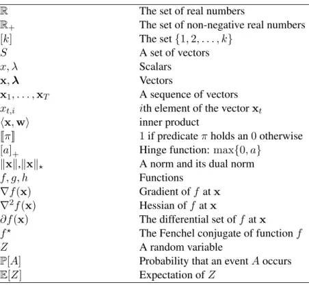
Table 1.1: Summary of notations.
R The set of real numbers
R+ The set of non-negative real numbers
[k] The set{1,2, . . . , k}
S A set of vectors
x, λ Scalars
x,λ Vectors
x1, . . . ,xT A sequence of vectors
xt,i ith element of the vectorxt
hx,wi inner product
[[π]] 1if predicateπholds an0otherwise [a]+ Hinge function: max{0, a}
kxk,kxk? A norm and its dual norm
f, g, h Functions
∇f(x) Gradient off atx
∇2f(x) Hessian off atx
∂f(x) The differential set off atx
f? The Fenchel conjugate of functionf
Z A random variable
P[A] Probability that an eventAoccurs
E[Z] Expectation ofZ
The inner product between vectorsxandwis denoted byhx,wi. Sets are designated by upper case letters (e.g. S). The set of real numbers is denoted by R and the set of non-negative real
numbers is denoted byR+. For anyk≥1, the set of integers{1, . . . , k}is denoted by[k]. Given a
predicateπ, we use the notation[[π]]to denote the function that outputs1ifπholds and0otherwise. The hinge function is denoted by[a]+= max{0, a}.
A norm of a vector xis denoted bykxk. The dual norm is defined as kλk? = sup{hx,λi :
kxk ≤1}. For example, the Euclidean norm,kxk2 = (hx,xi)1/2 is dual to itself and the`1norm,
kxk1 =P
i|xi|, is dual to the`∞norm,kxk∞= maxi|xi|.
Throughout the dissertation, we make extensive use of several notions from convex analysis. In the appendix we overview basic definitions and derive some useful tools. Here we summarize some of our notations. The gradient of a differentiable functionf is denoted by∇f and the Hessian is denoted by∇2f. Iff is non-differentiable, we denote its sub-differential set by∂f. We denote
the Fenchel conjugate of a functionf(w)byf?(θ) = supwhw,θi −f(w)(see SectionA.3in the appendix for more details).
CHAPTER 1. INTRODUCTION 9
denote the probability that an eventAoccurs. The expected value of a random variable is denoted byE[Z]. In some situations, we have a deterministic functionhthat receives a random variable as
input. We denote byE[h(Z)]the expected value of the random variableh(Z). Occasionally, we
omit the dependence ofhonZ. In this case, we clarify the meaning of the expectation by using the notationEZ[h].
Table1.1provides a summary of our notations.
1.6
Bibliographic Notes
How to predict rationally is a key issue in various research areas such as game theory, machine learning, and information theory. In this section we give a high level overview of related work in different research fields. The last section of each of the chapters below includes a detailed review of previous work relevant to the specific contents of each chapter.
In game theory, the problem of sequential prediction has been addressed in the context of playing repeated games with mixed strategies. A player who can achieve low regret (i.e. whose regret grows sublinearly with the number of rounds) is called a Hannan consistent player [63]. Hannan consistent strategies have been obtained by Hannan [63], Blackwell [9] (in his proof of the approachability theorem), Foster and Vohra [49,50], Freund and Schapire [55], and Hart and Mas-collel [64]. Von Neumann’s classical minimax theorem has been recovered as a simple application of regret bounds [55]. The importance of low regret strategies was further amplified by showing that if all players follow certain low regret strategies then the game converges to a correlated equilibrium (see for example [65,10]). Playing repeated games with mixed strategies is closely related to the expert setting widely studied in the machine learning literature [42,82,85,119].
Prediction problems have also intrigued information theorists since the early days of the in-formation theory field. For example, Shannon estimated the entropy of the English language by letting humans predict the next symbol in English texts [111]. Motivated by applications of data compression, Ziv and Lempel [124] proposed an online universal coding system for arbitrary in-dividual sequences. In the compression setting, the learner is not committed to a single prediction but rather assigns a probability over the set of possible outcomes. The success of the coding system is measured by the total likelihood of the entire sequence of symbols. Feder, Merhav, and Gutman [47] applied universal coding systems to prediction problems, where the goal is to minimize the number of prediction errors. Their basic idea is to use an estimation of the conditional probabilities of the outcomes given previous symbols, as calculated by the Lempel-Ziv coding system, and then to randomly guess the next symbol based on this conditional probability.
Another related research area is the “statistics without probability” approach developed by Dawid and Vovk [34,35], which is based on the theory of prediction with low regret.
CHAPTER 1. INTRODUCTION 10
In an attempt to unify different sequential prediction problems and algorithms, Cesa-Bianchi and Lugosi developed a unified framework called potential-based algorithms [19]. See also their inspiring book [20] about learning, prediction, and games. The potential-based decision strategy formulated by Cesa-Bianchi and Lugosi differs from our construction, which is based on online convex programming [123]. The analysis presented in [19] relies on a generalized Blackwell’s condition, which was proposed in [65]. This type of analysis is also similar to the analysis presented by [62] for the quasi-additive family of online learning algorithms. Our analysis is different and is based on the weak duality theorem, the generalized Fenchel duality, and strongly convex functions with respect to arbitrary norms.
Part I
Theory
Chapter 2
Online Convex Programming
2.1
Casting Online Learning as Online Convex Programming
In this chapter we formally define the setting of online learning. We then describe several as-sumptions under which the online learning setting can be cast as an online convex programming procedure.
Online learning is performed in a sequence of T consecutive rounds. On roundt, the learner is first given a question, cast as a vectorxt, and is required to provide an answer to this question.
For example,xt can be an encoding of an email message and the question is whether the email is
spam or not. The learner’s prediction is performed based on a hypothesis,ht:X → Y, whereX is
the set of questions andY is the set of possible answers. In the aforementioned example,Ywould be{+1,−1}where+1stands for a spam email and−1stands for a benign one. After predicting an answer, the learner receives the correct answer to the question, denotedyt, and suffers a loss
according to a loss function`(ht,(xt, yt)). The function`assesses the quality of the hypothesisht
on the example(xt, yt). Formally, let Hbe the set of all possible hypotheses, then`is a function
fromH ×(X × Y)into the reals. The ultimate goal of the learner is to minimize the cumulative loss he suffers along his run. To achieve this goal, the learner may choose a new hypothesis after each round so as to be more accurate in later rounds.
In most cases, the hypotheses used for prediction come from a parameterized set of hypotheses,
H={hw:w∈S}, whereSis a subset of a vector space. For example, the set of linear classifiers which is used for answering yes/no questions, is defined asH = {hw(x) = sign(hw,xi) : w ∈
Rn}. Thus, rather than saying that on round tthe learner chooses a hypothesis, we can say that
the learner chooses a parameter vectorwtand his hypothesis ishwt. Next, we note that once the
environment chooses a question-answer pair(xt, yt), the loss function becomes a function over the
hypothesis space or equivalently over the set of parameter vectors S. We can therefore redefine
CHAPTER 2. ONLINE CONVEX PROGRAMMING 13
the online learning process as follows. On roundt, the learner chooses a vectorwt ∈ S, which
defines a hypothesis hwt to be used for prediction. Then, the environment chooses a
question-answer pair(xt, yt), which induces the following loss function over the set of parameter vectors,
gt(w) =`(hw,(xt, yt)). Finally, the learner suffers the lossgt(wt) = `(hwt,(xt, yt)).
Let us further assume that the set of admissible parameter vectors, S, is convex and that the loss functionsgtare convex functions (for an overview of convex analysis see the appendix). Under
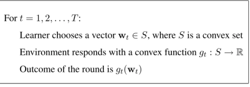
these assumptions, the online learning process can be described as an online convex programming procedure, defined as follows:
Fort= 1,2, . . . , T:
Learner chooses a vectorwt∈S, whereSis a convex set
Environment responds with a convex functiongt:S→R
Outcome of the round isgt(wt)
Figure 2.1: Online Convex Programming
In offline convex programming, the goal is to find a vectorwwithin a convex setSthat mini-mizes a convex objective function,g:S → R. In online convex programming, the setSis known
in advance, but the objective function may change along the online process. The goal of the online optimizer, which we call the learner, is to minimize the cumulative objective value
T
X
t=1
gt(wt) .
In summary, we have shown that the online learning setting can be cast as the task of online convex programming, assuming that:
1. The hypotheses used for prediction come from a parameterized set of hypotheses,H={hw:
w∈S}, whereSis a convex set.
2. The loss functions,gt(w) =`(hw,(xt, yt)), are convex functions with respect tow.
In Section2.3we discuss the case in which the second assumption above does not hold; namely, the loss functions are non-convex.
We conclude this section with a specific example in which the above assumptions clearly hold. The setting we describe is called online regression with squared loss. In online regression, the set of instances is then-dimensional Euclidean space,X =Rn, and the set of targets (possible answers)
CHAPTER 2. ONLINE CONVEX PROGRAMMING 14
is the reals,Y =R. The hypothesis set is
H={hw(x) =hw,xi |w∈Rn} ,
and thusS =Rn. The loss function is defined to be
`(hw,(x, y)) = (hw,xi −y)2 .
It is straightforward to verify thatS is a convex set and that for allt,gt(w) = `(hw,(xt, yt))is
convex with respect tow.
2.2
Regret
As mentioned earlier, the performance of an online learning algorithm is measured by the cumula-tive loss it suffers along its run on a sequence of examples(x1, y1), . . . ,(xT, yT). Ideally, we would
like to think of the correct answers as having been generated by an unknown yetfixedhypothesis
h such thatyt = h(xt)for allt ∈ [T]. Moreover, in a utopian case, the cumulative loss ofh on
the entire sequence is zero. In this case, we would like the cumulative loss of our online algorithm to be independent ofT. In the more realistic case there is noh that correctly predicts the correct answers of all observed instances. In this case, we would like the cumulative loss of our online algorithm not to exceed by much the cumulative loss ofanyfixed hypothesish. Formally, we assess the performance of the learner using the notion ofregret. Given any fixed hypothesish ∈ H, we define the regret of an online learning algorithm as the excess loss for not consistently predicting with the hypothesish,
R(h, T) = T X t=1 `(ht,(xt, yt))− T X t=1 `(h,(xt, yt)) .
Similarly, given any fixed vectoru ∈ S, we define the regret of an online convex programming procedure as the excess loss for not consistently choosing the vectoru∈S,
R(u, T) = T X t=1 gt(wt)− T X t=1 gt(u) .
In the next chapter, we present an algorithmic framework for online convex programming that guar-antees a regret of O(√T) with respect to any vector u ∈ S. Since we have shown that online learning can be cast as online convex programming, we also obtain a low regret algorithmic frame-work for online learning.
CHAPTER 2. ONLINE CONVEX PROGRAMMING 15
2.3
Non-convex loss functions and relative mistake bounds
In Section2.1we presented a reduction from online learning to online convex programming. This reduction is based on the assumption that for each roundt, the loss functiongt(w) =`(w,(xt, yt))
is convex with respect tow. A well known example in which this assumption does not hold is online classification with the 0-1 loss function. In this section we describe the mistake bound model, which extends the utilization of online convex programming to online learning with non-convex loss functions.
For simplicity and for historical reasons, we focus on binary classification problems, in which the set of instances isX = Rn and the set of possible answers isY = {+1,−1}. Extending the
technique presented below to general non-convex loss functions is straightforward. Define the hypothesis set of separating hyperplanes,
H={hw(x) =sign(hw,xi)|w∈Rn},
and the 0-1 loss function
`0-1(hw,(x, y)) = 1 if hw(x)6=y 0 if hw(x) =y
Therefore, the cumulative 0-1 loss of the online learning algorithm is the number of prediction mistakes the online algorithm makes along its run.
We now show that no algorithm can obtain a sub-linear regret bound for the 0-1 loss function. To do so, letX ={1}so our problem boils down to finding the bias of a coin in an online manner. An adversary can make the number of mistakes of any online algorithm to be equal toT, by simply waiting for the learner’s prediction and then providing the opposite answer as the true answer. In contrast, the number of mistakes of the constant prediction u = sign(P
tyt) is at most T /2.
Therefore, the regret of any online algorithm with respect to the 0-1 loss function will be at least
T /2.
To overcome the above hardness result, the common solution in the online learning literature is to find a convex loss function that upper bounds the original non-convex loss function. In binary classification, a popular convex loss function is the hinge-loss, defined as
`hinge(hw,(x, y)) = [1−yhw,xi]+ ,
CHAPTER 2. ONLINE CONVEX PROGRAMMING 16
and`hinge(hw,(x, y))≥`0-1(hw,(x, y)). Therefore, for anyu∈Swe have
R(u, T) = T X t=1 `hinge(hwt,(xt, yt))− T X t=1 `hinge(hu,(xt, yt)) ≥ T X t=1 `0-1(hwt,(xt, yt))− T X t=1 `hinge(hu,(xt, yt)) .
As a direct corollary from the above inequality we get that a low regret algorithm for the (convex) hinge-loss function can be utilized for deriving an online learning algorithm for the 0-1 loss with the bound T X t=1 `0-1(hwt,(xt, yt)) ≤ T X t=1 `hinge(hu,(xt, yt)) +R(u, T) .
Denote by M the set of rounds in whichhwt(xt) 6= yt and note that the left-hand side of the
above is equal to|M|. Furthermore, we can remove the examples not inMfrom the sequence of examples, and obtain a bound of the form
|M| ≤ X
t∈M
`hinge(hu,(xt, yt)) +R(u,|M|) . (2.1)
Such bounds are called relative mistake bounds.
In the next chapter, we present a low regret algorithmic framework for online learning. In particular, this framework yields an algorithm for online learning with the hinge-loss that attains the regret bound R(u, T) = Xkuk√T, whereX = maxtkxtk. Running this algorithm on the
examples inMresults in the famous Perceptron algorithm [95]. Combining the regret bound with Eq. (2.1) we obtain the inequality
|M| ≤ X
t∈M
`hinge(hu,(xt, yt)) +Xkuk
p
|M|,
which implies that (see Lemma19in SectionA.5)
|M| ≤ X t∈M `hinge(hu,(xt, yt)) +Xkuk s X t∈M `hinge(hu,(xt, yt)) +X2kuk2 .
The bound we have obtained is the best relative mistake bound known for the Perceptron algo-rithm [58,103,106].
CHAPTER 2. ONLINE CONVEX PROGRAMMING 17
2.4
Bibliographic notes
The term “online convex programming” was introduced by Zinkevich [123] but this setting was introduced some years earlier by Gordon in [60]. This model is also closely related to the model of relative loss bounds presented by Kivinen and Warmuth [76,75,77]. Our presentation of relative mistake bounds follows the works of Littlestone [84], and Kivinen and Warmuth [76].
The impossibility of obtaining a regret bound for the 0-1 loss function dates back to Cover [26], who showed that any online predictor that makesdeterministicpredictions cannot have a vanishing regret universally for all sequences. One way to circumvent this difficulty is to allow the online predictor to make randomized predictions and to analyze its expected regret. In this dissertation we adopt another way and follow the mistake bound model, namely, we slightly modify the regret-based model in which we analyze our algorithm.
Chapter 3
Low Regret and Duality
3.1
Online Convex Programming by Incremental Dual Ascend
In this chapter we present a general low regret algorithmic framework for online convex program-ming. Recall that the regret of an online convex programming procedure for not consistently choos-ing the vectoru∈Sis defined to be,
R(u, T) = T X t=1 gt(wt)− T X t=1 gt(u) . (3.1)
We derive regret bounds that take the following form
∀u∈S, R(u, T) ≤ (f(u) +L)
√
T , (3.2)
wheref :S →R+andL∈R+. Informally, the functionf measures the “complexity” of vectors inSand the scalarLis related to some generalized Lipschitz property of the functionsg1, . . . , gT.
We defer the exact requirements we impose onf andLto later sections.
Our algorithmic framework emerges from a representation of the regret bound given in Eq. (3.2) using an optimization problem. Specifically, we rewrite Eq. (3.2) as follows
T X t=1 gt(wt) ≤ inf u∈S T X t=1 gt(u) + (f(u) +L) √ T . (3.3)
That is, the learner’s cumulative loss should be bounded above by the minimum value of an op-timization problem in which we jointly minimize the cumulative loss ofu and the “complexity” ofu as measured by the functionf. Note that the optimization problem on the right-hand side of
CHAPTER 3. LOW REGRET & DUALITY 19
Eq. (3.3) can only be solved in retrospect after observing the entire sequence of loss functions. Nev-ertheless, writing the regret bound as in Eq. (3.3) implies that the learner’s cumulative loss forms a lower bound for a minimization problem.
The notion of duality, commonly used in convex optimization theory, plays an important role in obtaining lower bounds for the minimal value of a minimization problem (see for example [89]). By generalizing the notion of Fenchel duality, we are able to derive a dual optimization problem. While the primal minimization problem of finding the best vector inScan only be solved in hindsight, the dual problem can be optimized incrementally, as the online learning progresses. In order to derive explicit quantitative regret bounds we make immediate use of the fact that dual objective lower bounds the primal objective. We therefore reduce the process of online convex optimization to the task of incrementally increasing the dual objective function. The amount by which the dual increases serves as a new and natural notion of progress. By doing so we are able to link the primal objective value, the learner’s cumulative loss, and the increase in the dual.
3.2
Generalized Fenchel Duality
In this section we derive our main analysis tool. First, it should be recalled that the Fenchel conju-gate of a functionf is the function (see SectionA.3)
f?(θ) = sup w∈S
hw,θi −f(w) .
In the following, we derive the dual problem of the following optimization problem,
inf w∈S f(w) + T X t=1 gt(w) ! . An equivalent problem is inf w0,w1,...,wT f(w0) + T X t=1 gt(wt) ! s.t. w0∈S and ∀t∈[T], wt=w0 .
IntroducingTvectorsλ1, . . . ,λT, eachλt∈Rnis a vector of Lagrange multipliers for the equality
constraintwt=w0, we obtain the following Lagrangian
L(w0,w1, . . . ,wT,λ1, . . . ,λT) = f(w0) + T X t=1 gt(wt) + T X t=1 hλt,w0−wti .
CHAPTER 3. LOW REGRET & DUALITY 20
The dual problem is the task of maximizing the following dual objective value,
D(λ1, . . . ,λT) = inf w0∈S,w1,...,wT L(w0,w1, . . . ,wT,λ1, . . . ,λT) = − sup w0∈S hw0,− T X t=1 λti −f(w0) ! − T X t=1 sup wt (hwt,λti −gt(wt)) = −f? − T X t=1 λt ! − T X t=1 g?t(λt) ,
wheref?, g1?, . . . , gT? are the Fenchel conjugate functions off, g1, . . . , gT. Therefore, the
general-ized Fenchel dual problem is
sup λ1,...,λT −f? − T X t=1 λt ! − T X t=1 g?t(λt) . (3.4)
Note that whenT = 1the above duality is the so-called Fenchel duality [11].
3.3
A Low Regret Algorithmic Framework for Online Convex
Pro-gramming
In this section we describe a template learning algorithm for online convex programming. Recall that we would like our learning algorithm to achieve a regret bound of the form given in Eq. (3.3). We start by rewriting Eq. (3.3) as follows
T X t=1 gt(wt)−c L ≤ inf u∈S c f(u) + m X t=1 gt(u) ! , (3.5)
wherec =√T. Thus, up to the sublinear termc L, the learner’s cumulative loss lower bounds the optimum of the minimization problem on the right-hand side of Eq. (3.5). Based on the previous section, the generalized Fenchel dual function of the right-hand side of Eq. (3.5) is
D(λ1, . . . ,λT) = −c f? −1c T X t=1 λt ! − T X t=1 g?t(λt) , (3.6)
where we used the fact that the Fenchel conjugate ofc f(w)is−cf?(θ/c)(see SectionA.3.1).
Our construction is based on the weak duality theorem stating that any value of the dual problem is smaller than the optimal value of the primal problem. The algorithmic framework we propose is
CHAPTER 3. LOW REGRET & DUALITY 21
therefore derived by incrementally ascending the dual objective function. Intuitively, by ascending the dual objective we move closer to the optimal primal value and therefore our performance be-comes similar to the performance of the best fixed weight vector which minimizes the right-hand side of Eq. (3.5).
Our algorithmic framework utilizes the following important property of the dual function given in Eq. (3.6): Assume that for alltwe haveinfwgt(w) = 0and thus the definition ofg?t implies that
g?t(0) = 0. Then, for any sequence oftvectors(λ1, . . . ,λt)we have
D(λ1, . . . ,λt,0, . . . ,0) = −c f? −1c X i≤t λi − X i≤t g?(λi) .
That is, if the tail of dual solutions is grounded to zero then the dual objective function does not depend on theyet to be seentail of functionsgt+1, . . . , gT. This contrasts with the primal objective
function where we must know all the functionsg1, . . . , gT for calculating the primal objective value
at some vectorw.
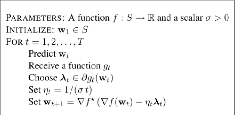
Based on the above property, we initially use the elementary dual solution λ1t = 0 for all t. Sincef serves as a measure of “complexity” of vectors in S we enforce the requirement that the minimum offover the vectors inSis zero. From this requirement we get thatD(λ11, . . . ,λ1T) = 0. We assume in addition thatf is strongly convex (see Definition4in SectionA.4). Therefore, based on Lemma15in SectionA.4, the functionf? is differentiable. At roundt, the learner predicts the vector wt = ∇f? − 1 c T X i=1 λti ! . (3.7)
After predictingwt, the environment responds with the functiongtand the learner suffers the loss
gt(wt). Finally, the learner finds a new set of dual variables as follows. Denote by∂tthe differential
set ofgtatwt, that is,
∂t = {λ : ∀w∈S, gt(w)−gt(wt) ≥ hλ,w−wti} . (3.8)
The new dual variables(λt+11 , . . . ,λt+1T )are set to beanyset of vectors that satisfy the condition:
∃λ0 ∈∂t s.t. D(λt+11 , . . . ,λ t+1
T ) ≥ D(λ t
1, . . . ,λtt−1,λtt+λ0,λtt+1, . . . ,λtT) . (3.9)
In practice, we cannot calculate the dual objective value at the end of roundtunless the lastT−t
dual vectors are still grounded to zero. In this case, we can rewrite Eq. (3.9) as follows
CHAPTER 3. LOW REGRET & DUALITY 22
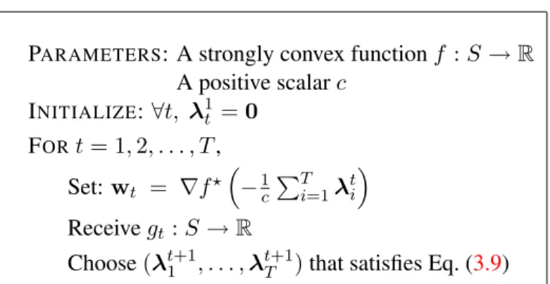
PARAMETERS: A strongly convex functionf :S→R
A positive scalarc INITIALIZE:∀t, λ1t =0 FORt= 1,2, . . . , T, Set:wt = ∇f? −1 c PT i=1λti Receivegt:S→R
Choose(λt+11 , . . . ,λt+1T )that satisfies Eq. (3.9)
Figure 3.1: An Algorithmic Framework for Online Convex Programming
Put another way, the increase in the dual objective due to the update step must be at least as large as the increase that would have been obtained had we only set thetvariable to beλ0instead of its previous value of zero.
A summary of the algorithmic framework is given in Figure3.1. In the next section we show that the above condition ensures that the increase of the dual at roundtis proportional to the loss
gt(wt).
We conclude this section with two update rules that trivially satisfy the above condition. The first update scheme simply findsλ0 ∈∂tand set
λt+1i = (
λ0 ifi=t
λti ifi6=t . (3.11)
The second update defines
(λt+11 , . . . ,λt+1T ) = argmax
λ1,...,λT
D(λ1, . . . ,λT) s.t. ∀i6=t, λi=λti . (3.12)
3.4
Analysis
In this section we analyze the performance of the template algorithm given in the previous section. Our proof technique is based on monitoring the value of the dual objective function. The main result is the following lemma which upper and lower bounds the final value of the dual objective function.
Lemma 1 Letf be a strongly convex function with respect to a normk · kover a setSand assume thatminw∈Sf(w)≥0. Letk · k?be the dual norm ofk · k. Letg1, . . . , gT be a sequence of convex
CHAPTER 3. LOW REGRET & DUALITY 23
given in Figure3.1is run on this sequence with the function f. Let w1, . . . ,wT be the sequence
of primal vectors that the algorithm generates and λT1+1, . . . ,λTT+1 be its final sequence of dual variables. Then, there exists a sequence of sub-gradientsλ01, . . . ,λ0T, whereλ0t∈∂tfor allt, such
that T X t=1 gt(wt)− 1 2c T X t=1 kλ0tk2? ≤ D(λ1T+1, . . . ,λTT+1) ≤ inf w∈Sc f(w) + T X t=1 gt(w) .
Proof The second inequality follows directly from the weak duality theorem. Turning to the left most inequality, we first note that the assumptionminw∈Sf(w)≥0implies that
f?(0) = max
w∈Shw,0i −f(w) = −wmin∈Sf(w)≤0 .
Similarly, for alltwe havegt?(0)≤0, and thusD(0, . . . ,0)≥0. Denote
∆t = D(λt+11 , . . . ,λTt+1)− D(λt1, . . . ,λtT)
and note thatD(λT1+1, . . . ,λTT+1)can be rewritten as
D(λT1+1, . . . ,λTT+1) = T X t=1 ∆t +D(λ11, . . . ,λ1T) ≥ T X t=1 ∆t . (3.13)
The condition on the update of the dual variables given in Eq. (3.9) implies that
∆t ≥ D(λt1, . . . ,λtt−1,λtt+λ0t,λtt+1, . . . ,λtT)− D(λt1, . . . ,λtt−1,λtt,λtt+1, . . . ,λtT) (3.14)
for some subgradientλ0t ∈∂t. Denotingθt =−1cPTj=1λtj and using the definition ofD, we can
rewrite Eq. (3.14) as,
∆t ≥ −c f?(θt−λ0t/c)−f?(θt)
−gt?(λ0t) .
Lemma15in SectionA.4tells us that iff is a strongly convex function w.r.t. a normk · kthen for any two vectorsµ1andµ2we have
f?(µ1+µ2)−f?(µ1)≤ h∇f?(µ1),µ2i+12kµ2k2
? . (3.15)
Using this lemma and the definition ofwtwe get that
∆t ≥ h∇f?(θt),λ0ti −gt?(λ0t)− 1 2ckλ 0 tk2? = hwt,λt0i −gt?(λ0t)− 1 2ckλ 0 tk2? . (3.16)
CHAPTER 3. LOW REGRET & DUALITY 24
Since λ0t ∈ ∂t and since we assume thatgtis closed and convex, we can apply Lemma11 from
Section A.3to get that hwt,λ0ti −gt?(λ 0
t) = gt(wt). Plugging this equality into Eq. (3.16) and
summing overtwe obtain that
T X t=1 ∆t ≥ T X t=1 gt(wt)− 1 2c T X t=1 kλ0tk2? .
Combining the above inequality with Eq. (3.13) concludes our proof.
Rearranging the inequality in Lemma1we obtain that
∀u∈S, R(u, T) ≤ c f(u) + 1 2c T X t=1 kλ0tk2? . (3.17)
To derive a regret bound from the above inequality we need to bound the cumulative sum ofkλ0tk2 ?.
Let us first assume thatk · k?is the Euclidean norm. In this case, we can boundkλ0tkby assuming
thatgtis a Lipschitz continuous function. More generally, let us define
Definition 1 A functiong:S →RisL-Lipschitz with respect to a normk · kif
∀w∈S, ∀λ∈∂g(w), kλk? ≤L .
The following regret bound follows as a direct corollary of Lemma1.
Corollary 1 Under the same conditions of Lemma1. Assume that there exists a constantLsuch that for allt, the functiongtis
√
2L-Lipschitz with respect to the normk · k?. Then, for allu ∈S
we have, R(u, T) = T X t=1 gt(wt)− T X t=1 gt(u) ≤ c f(u) + L T c .
In particular, for any constantU > 0, settingc = pT L/U yields the regret bound R(u, T) ≤
f(u)/√U +√U
√
L T. Furthermore, iff(u)≤U thenR(u, T) ≤ 2√L U T .
The second regret bound we derive is based on a different bound on the norm of sub-gradients. We first need the following definition:
Definition 2 A functiong:S →RisL-self-bounded with respect to a normk · kif
∀w∈S, ∃λ∈∂g(w), 1
2kλk
2
CHAPTER 3. LOW REGRET & DUALITY 25
Based on the above definition, we are ready to state our second regret bound.
Theorem 1 Under the same conditions of Lemma1. Assume that there exists a constantLsuch that for allt, the functiongtisL-self-bounded with respect to the normk · k?. LetU1andU2be two
positive scalars and setc =L+pL2+L U
2/U1. Then, for anyu ∈S that satisfiesf(u)≤ U1
andPT t=1gt(u)≤U2 we have, R(u, T) = T X t=1 gt(wt)− T X t=1 gt(u) ≤ 2 p L U1U2+ 4L U1 .
Proof Combining Eq. (3.17) with the assumption that{gt}areL-self-bounded yields T X t=1 gt(wt)− T X t=1 gt(u) ≤ cf(u) + L c T X t=1 gt(wt).
Rearranging the above we get that
T X t=1 gt(wt)− T X t=1 gt(u) ≤ c 1−Lc f(u) + 1 1−Lc −1 ! T X t=1 gt(u).
Using the assumptionsf(u)≤U1andPTt=1gt(u)≤U2we obtain
R(u, T) ≤ c U1 1−Lc + 1 1−Lc −1 ! U2 = U2 c L−1 1 + c 2 L2 U1L U2 .
Plugging the definition ofcinto the above gives
R(u, T) ≤ q U2 1 + U2 U1L 1 + 1 + r 1 + U2 U1L !2 U1L U2 = q U2 1 + U2 U1L 1 + 2 + 2 r 1 + U2 U1L + U2 U1L ! U1L U2 ! = q 2U2 1 + U2 U1L +q2U1L 1 + U2 U1L + 2U1L ≤ q 2U2 1 + U2 U1L + 4U1L = 2U2 q U1L U2 q U1L U2 + 1 + 4U1L ≤ 2pU1U2L+ 4U1L .
CHAPTER 3. LOW REGRET & DUALITY 26
The regret bound in Theorem1will be small if there existsufor which bothf(u)andP
tgt(u)
are small. In particular, settingU1to be a constant andU2 =
√
T we obtain thatR(u, T)≤O(√T). Note that the bound can be much better if there existsuwithP
tgt(u)
√
T. Unfortunately, to benefit from this case we must know the upper bound U2 in advance (since c depends on U2).
Similarly, in Corollary1the definition ofcdepends on the horizonT. In Section3.5we propose a method that automatically tunes the parametercas the online learning progresses.
3.5
Automatically tuning the complexity tradeoff parameter
In the previous sections we described and analyzed an algorithmic framework for online convex programming that achieves low regret provided that the parameter c is appropriately tuned. In this section, we present methods for automatically tuning the parameter cas the online learning progresses.
We start by writing an instantaneous objective function
Pt(w) =ctf(w) +
X
t
gt(w),
where0 < c1 ≤c2 ≤. . .. Using the generalized Fenchel duality derived in Section3.2we obtain
that the dual objective ofPtis
Dt(λ1, . . . ,λT) =−ctf? − 1 ct T X t=1 λt ! − T X t=1 gt?(λt) .
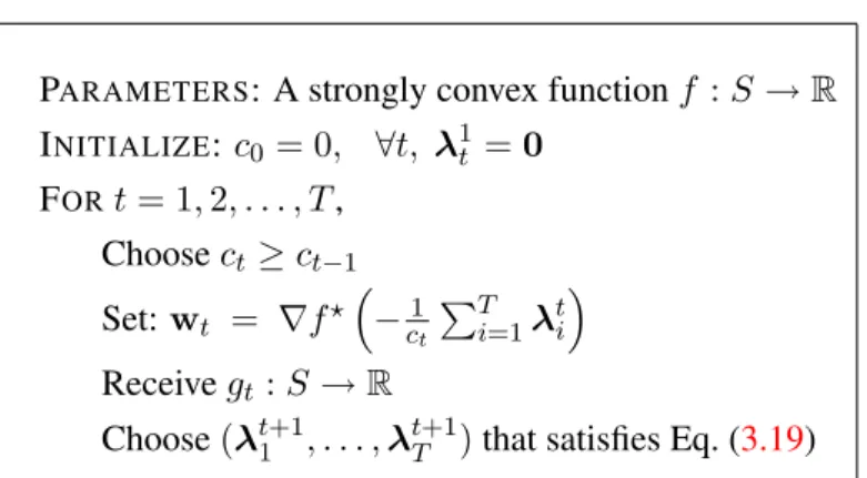
We now describe an algorithmic framework for online convex programming in which the pa-rametercis changed from round to round. Initially, we defineλ11 =. . .=λ1T =0andc0 = 0. At
each round of the online algorithm we choosect≥ct−1and setwtto be
wt = ∇f? − 1 ct X i λti ! . (3.18)
At the end of each online round, we set the new dual variables(λt+11 , . . . ,λt+1T )to be any set of vectors that satisfy the condition:
∃λ0 ∈∂t s.t. Dt(λt+11 , . . . ,λ t+1
CHAPTER 3. LOW REGRET & DUALITY 27
PARAMETERS: A strongly convex functionf :S→R
INITIALIZE:c0= 0, ∀t, λ1t =0 FORt= 1,2, . . . , T, Choosect≥ct−1 Set:wt = ∇f? −c1 t PT i=1λ t i Receivegt:S→R
Choose(λt+11 , . . . ,λt+1T )that satisfies Eq. (3.19)
Figure 3.2: An Algorithmic Framework for Online Convex Programming with a variable learning rate.
The algorithmic framework is summarized in Figure3.2.
The following lemma generalizes Lemma1to the case wherecvaries as learning progresses. Lemma 2 Let f be a strongly convex function with respect to a norm k · k over a set S and let
k · k? be the dual norm ofk · k. Assume thatminw∈Sf(w) ≥0. Letg1, . . . , gT be a sequence of
convex and closed functions, such thatinfwgt(w) ≥0for allt ∈ [T]. Assume that an algorithm
of the form given in Figure3.2is run on this sequence with the functionf. Letw1, . . . ,wT be the
sequence of primal vectors that the algorithm generates andλT1+1, . . . ,λTT+1be its final sequence of dual variables. Then, there exists a sequence of sub-gradientsλ01, . . . ,λ0T, whereλ0t∈∂tfor all
t, such that ∀u∈S, T X t=1 gt(wt)− T X t=1 gt(u) ≤ cT f(u) + 1 2 T X t=1 kλ0tk2 ? ct .
Proof We prove the lemma by boundingDT(λT1+1, . . . ,λTT+1)from above and below. The upper bound DT(λT1+1, . . . ,λTT+1) ≤ cTf(u) + T X t=1 gt(u) , (3.20)
follows directly from the weak duality theorem. Turning to derive a lower bound, we denote
∆t=Dt(λt+11 , . . . ,λt+1T )− Dt−1(λt1, . . . ,λtT),
where for simplicity we setD0=D1. We can now rewrite,
DT(λT1+1, . . . ,λTT+1) = T X t=1 ∆t +D0(λ11, . . . ,λ1T) ≥ T X t=1 ∆t , (3.21)
CHAPTER 3. LOW REGRET & DUALITY 28
where the last inequality follows from the assumptions,minw∈Sf(w)≥0andminw∈Sgt(w)≥0.
Lemma12in SectionA.3tells us that conjugate functions preserve order. If a functionf1is always
greater than a functionf2thenf1?≤f2?. Combining this fact with the assumptionct≥ct−1implies
that for anyθ,ctf?(−θ/ct)≤ct−1f?(−θ/ct−1)and thus the definition ofDyields that
Dt(λ1, . . . ,λT)≥ Dt−1(λ1, . . . ,λT) .
Therefore,
∆t≥ Dt(λt+11 , . . . ,λt+1T )− Dt(λt1, . . . ,λtT).
As in the proof of Lemma1, using the definition ofwt, Lemma15and Lemma11we get that
∆t≥gt(wt)−
1 2ct
kλ0tk2 ?.
We conclude our proof by summing overtand combining with Eq. (3.21) and Eq. (3.20).
Choosing for example ct ∝
√
t and using the inequalityPT
t=11/
√
t ≤ 2√T we obtain the following:
Corollary 2 Under the same conditions of Lemma2. Assume that there exists a constantLsuch that for allt, the functiongtis
√
2L-Lipschitz with respect to the normk · k?. LetU >0be a scalar and for alltsetct=
p
t L/U. Then, for allu∈Swe have,
R(u, T) ≤ 2 f(u)/ √ U + √ U √ L T . Furthermore, iff(u)≤U thenR(u, T) ≤ 4√L U T .
The above corollary assumes that the Lipschitz constantLis known in advance. In some situations, the Lipschitz constant of each function gt is known only at the beginning of round t (although
the function itself is only revealed at the end of round t). This will be the case for example in online learning with the hinge-loss, where the Lipschitz constant depends on the instance whereas the functiongt also depends on the unknown label. The following corollary gives an improved
parameter selection for this case.
Corollary 3 Under the same conditions of Lemma2. Assume that for allt, the functiongtis
√
2Lt
-Lipschitz with respect to the normk · k?, whereLt is known to the algorithm at the beginning of
roundt. DenoteL = maxtLt. Let U > 0 be a scalar and for alltset ct =
p
CHAPTER 3. LOW REGRET & DUALITY 29
Then, for allu∈Swe have,
R(u, T) ≤ 2f(u)/√U +√U√L T .
Furthermore, iff(u)≤U thenR(u, T) ≤ 4√L U T .
Next, we turn to deriving a regret bound analogous to the bound in Theorem1, without assuming prior knowledge of the parameterU2. We first need the following technical lemma.
Lemma 3 Let0 =a0 ≤a1≤. . .≤aT be a sequence of scalars and denoteA= maxt(at−at−1).
Then, for anyβ≥1we have
T X t=1 at−at−1 p β+at−1 ≤ 2p1 +A/β(pβ+aT − p β) .
Proof Using Holder inequality, we get that
T X t=1 at−at−1 p β+at−1 = T X t=1 at−at−1 √ β+at s β+at β+at−1 ≤ max t s β+at β+at−1 ! T X t=1 a√t−at−1 β+at ! .
Next, we note that
T X t=1 at−at−1 √ β+at ≤ Z aT 0 1 √ β+xdx = 2( p β+aT − p β+ 0) .
Finally, for alltwe have
β+at β+at−1 = 1 +at−at−1 β+at−1 ≤ 1 +at−at−1 β ≤ 1 +A/β .
Combining the above three equations we conclude our proof.
Based on the above lemma, we are ready to provide a regret bound for self-bounded functions. Theorem 2 Under the same conditions of Lemma2. Assume that there exists a constantLsuch that for allt, the function gt is L-self-bounded with respect to the norm k · k?. Let β1 ≥ 1and
CHAPTER 3. LOW REGRET & DUALITY 30
β2 >0be two scalars, and for alltdefine
ct=β2 s β1+ X i<t gi(wi) .
DenoteG= 2p1 + maxtgt(wt)/β1. Then, for allu∈Swe have,
R(u, T) ≤ β2f(u) + LG β2 T X t=1 gt(u) +β1 !12 + β2f(u) + LG β2 2 .
Proof Combining the assumption that{gt}areL-self-bounded with Lemma2gives that
R(u, T) ≤ cTf(u) +L T X t=1 gt(wt) ct . (3.22)
Denoteat=Pi≤tgi(wi)and note thatat−at−1 =gt(wt). Using Lemma3and the definition of
ctwe get that T X t=1 gt(wt) ct ≤ 2 β2 q aT(1 + max i gi(wi)/β1) = G β2 √ aT ≤ G β2 p β1+aT .
Combining the above with Eq. (3.22), using the fact thatcT ≤β2
√
β1+aT, and rearranging terms
we obtain that (β1+aT)− β2f(u) + LG β2 p β1+aT − T X t=1 gt(u) +β1 ! ≤ 0 .
The above inequality holds only if (see Lemma19in SectionA.5)
β1+aT ≤ T X t=1 gt(u) +β1+ β2f(u) + LG β2 2 + β2f(u) + LG β2 v u u t T X t=1 gt(u) +β1.
Rearranging the above concludes our proof.
The regret bound in the above theorem depends on the variable G, which depends on the maximal value of gt(wt). To ensure that gt(wt) is bounded, one can restrict the set S so that
maxw∈Sgt(w) will be bounded. In this case, we can set β1 to be maxtmaxw∈Sgt(w), which
CHAPTER 3. LOW REGRET & DUALITY 31
Corollary 4 Under the same conditions of Theorem2. Assume that for alltmaxw∈Sgt(w) ≤β1
and thatmaxw∈Sf(w)≤U. Setβ2 = 8 1 4 pL/U. Then, R(u, T) ≤ 3.4 √ L U T X t=1 gt(u) +β1 !12 + 11.4L U .
3.6
Tightness of regret bounds
In the previous sections we presented algorithmic frameworks for online convex programming with regret bounds that depend on√T and on the complexity of the competing vector as measured by
f(u). In this section we show that without imposing additional conditions our bounds are tight, in a sense that is articulated below.
First, we study the dependence of the regret bounds on√T.
Theorem 3 For any online convex programming algorithm, there exists a sequence of1-Lipschitz convex functions of lengthT such that the regret of the algorithm on this sequence with respect to a vectoruwithkuk2≤1isΩ(
√
T).
Proof The proof is based on the probabilistic method [2]. LetS = [−1,1]andf(w) = 12w2. We clearly have thatf(w)≤1/2for allw∈S. Consider a sequence of linear functionsgt(w) =σtw
whereσ ∈ {+1,−1}. Note thatgtis1-Lipschitz for allt. Suppose that the sequenceσ1, . . . , σT is
chosen in advance, independently with equal probability. Sincewtonly depends onσ1, . . . , σt−1it
is independent ofσt. Thus,Eσt[gt(wt)|σ1, . . . , σt−1] = 0. On the other hand, for anyσ1, . . . , σT
we have that min u∈S T X t=1 gt(u) ≤ − T X t=1 σt . Therefore, Eσ1,...,σT[R(u, T)] = Eσ1,...,σT[ X t gt(wt)]−Eσ1,...,σT[min u X t gt(u)] ≥ 0 +Eσ1,...,σT " |X t σt| # .
The right-hand side above is the expected distance afterT steps of a random walk and is thus equal approximately top2T /π= Ω(√T)(see for example [88]). Our proof is concluded by noting that if the expected value of the regret is greater thanΩ(√T), then there must exist at least one specific sequence for which the regret is greater thanΩ(√T).
CHAPTER 3. LOW REGRET & DUALITY 32
Next, we study the dependence on the complexity functionf(w).
Theorem 4 For any online convex programming algorithm, there exists a strongly convex function
f with respect to a normk · k, a sequence of1-Lipschitz convex functions with respect tok · k?, and
a vectoru, such that the regret of the algorithm on this sequence isΩ(f(u)).
Proof Let S = RT and f(w) = 12kwk22. Consider the sequence of functions in which
gt(w) = [1−ythw,eti]+ where yt ∈ {+1,−1} and et is the tth vector of the standard base,
namely, et,i = 0 for all i 6= t andet,t = 1. Note that gt(w) is1-Lipschitz with respect to the
Euclidean norm. Consider any online learning algorithm. If on roundt we have wt,i ≥ 0 then
we set yt = −1and otherwise we setyt = 1. Thus,gt(wt) ≥ 1. On the other hand, the vector
u= (y1, . . . , yT)satisfiesf(u)≤T /2andgt(u) = 0for allt. Thus,R(u, T)≥T = Ω(f(u)).
3.7
Bibliographic notes
We presented a new framework for designing and analyzing algorithms for online convex program-ming. The usage of duality for the design of online algorithms was first proposed in [106, 107], in the context of binary classification with the hinge-loss. The generalization of the framework to online convex programming is based on [104]. The self-tuning version we presented in Section3.5 is new. Specific self-tuning online algor