One plus one can be greater than two: Evaluating synergies of development programmes in Malawi

Full Terms & Conditions of access and use can be found at

http://www.tandfonline.com/action/journalInformation?journalCode=fjds20

Download by: [168.202.253.225] Date: 16 October 2017, At: 08:47

The Journal of Development Studies

ISSN: 0022-0388 (Print) 1743-9140 (Online) Journal homepage: http://www.tandfonline.com/loi/fjds20

One Plus One can be Greater than Two: Evaluating

Synergies of Development Programmes in Malawi

Noemi Pace, Silvio Daidone, Benjamin Davis, Sudhanshu Handa, Marco

Knowles & Robert Pickmans

To cite this article: Noemi Pace, Silvio Daidone, Benjamin Davis, Sudhanshu Handa, Marco Knowles & Robert Pickmans (2017): One Plus One can be Greater than Two: Evaluating Synergies of Development Programmes in Malawi, The Journal of Development Studies, DOI: 10.1080/00220388.2017.1380794

To link to this article: http://dx.doi.org/10.1080/00220388.2017.1380794

Published online: 08 Oct 2017.

Submit your article to this journal

Article views: 33

View related articles

One Plus One can be Greater than Two: Evaluating

Synergies of Development Programmes in Malawi

NOEMI PACE*

**, SILVIO DAIDONE**, BENJAMIN DAVIS

, SUDHANSHU HANDA

,

MARCO KNOWLES**

& ROBERT PICKMANS

*Department of Economics, University Ca’Foscari of Venice, Venezia, Italia, **Social Policies and Rural Institutions Division

(ESP), Food and Agriculture Organization of the United Nations (FAO), Rome, Italy,†Food and Agriculture Organization of the

United Nations (FAO), Rome, Italy,‡Department of Public Policy, University of North Carolina at Chapel Hill, Chapel Hill, NC,

USA,§_{Department of Agricultural and Resource Economics, University of Berkeley, Berkeley, CA, USA}

(Original version submitted July 2016; Final version accepted August 2017)

ABSTRACT This paper investigates the interplay between the Social Cash Transfer Programme (SCTP) and the Farm Input Subsidy Programme (FISP) in Malawi. We take advantage of data collected from a 17-month evaluation of a sample of households eligible to receive SCTP, which also provided information about inclusion into FISP. We estimate two types of synergies: i) the complementarity between SCTP and FISP, that is whether the impact of both interventions run together is larger than the sum of the impacts of these interventions when run separately, and ii) the incremental impact of receiving FISP when a household already receives SCTP, as well as the incremental impact of receiving SCTP when a household already receives FISP. The analysis shows that there are synergies between the two policy interventions, mainly in terms of incremental impacts of each programme over the other, in increasing expenditure, agricultural production and livestock.

1. Introduction

There is a growing body of literature on the impacts of policy interventions implemented in develop-ing countries to tackle hunger and poverty in the short and long run. These programmes include cash transfers, food, supplements, provision of subsidies for agricultural inputs and activities, provision of information and training sessions on matters broadly related to education and health. It is plausible that there are interactions between these programmes, yet programme evaluators are generally only able to estimate the stand-alone impact of each programme without much attention to the potential synergies and degree of complementarity between them. However, this kind of analysis is relevant for several reasons. First, resources are scarce: it is necessary to run programmes that reinforce each other rather than programmes that reciprocally reduce their effectiveness. Second, if the synergies and the degree of complementarity is high and significant, policy-makers could in principle reduce the resources allocated to various programmes to reach the same desired results. Third, if the degree of substitut-ability is high and significant, policy-makers should carefully prioritise desired outcomes and define a realistic timeline to avoid‘crowding out’the effects of the various programmes.

This paper focuses on the experience of a sub-Saharan country, Malawi, in which in recent years the Social Cash Transfer Programme (SCTP) and the Farm Input Subsidy Programme (FISP) have been

Correspondence Address: Noemi Pace, Department of Economics, University Ca’Foscari of Venice, Cannaregio, 873,

30121, Venezia, Italia. Email:[email protected];[email protected]

Supplementary Materials are available for this article which can be accessed via the online version of this journal athttps://doi.

org/10.1080/00220388.2017.1380794

https://doi.org/10.1080/00220388.2017.1380794

© 2017 Informa UK Limited, trading as Taylor & Francis Group

implemented simultaneously as instruments for reducing poverty and vulnerability to hunger among poor households that mostly rely on agriculture as their main source of income.

FISP and SCTP are expected to have impacts on several outcomes. The FISP is expected to directly influence production decisions, but its contribution towards reducing hunger and poverty is mediated by factors such as access to land, water and labour for food production, responsiveness of yields to increased inputs, climatic factors, and the relative position of small poor farmers as net buyers or net sellers of grains in food markets. The SCTP is a welfare intervention that acts directly on the consumption capability of the recipients: the additional cash can be used directly to increase both quantity and quality of food. Recipients of the cash can, in addition, use this for purchasing productive inputs and assets. Several prior studies focus on the isolated impact of SCTP (Asfaw, Pickmans, & Davis, 2015; Covarrubias, Davis, & Winters, 2012; Handa, Angeles, Abdoulayi, Mvula, & Tsoka, 2015b) and FISP in Malawi (among others, Arndt, Pauw, & Thurlow,2016; Chirwa & Dorward,2013; Dorward et al.,2013; Jayne & Ricker-Gilbert,2011).

This paper is the first attempt to shed light on the interplay between FISP and SCTP using survey data. More specifically, the paper investigates the impacts on poor and ultra-poor house-holds when they participate in either FISP or SCTP alone or when they participate in both programmes simultaneously. We focus on a variety of outcomes, including household expenditure (food and non-food), food security and on contributing outcomes such as productive activities (crop production, input use) and livestock. In assessing the impacts of the two combined inter-ventions, we focus on two types of synergies: i) the complementarity between SCTP and FISP, that is whether the impact of both interventions run together is larger than the sum of the impacts of these interventions when run separately; ii) the incremental impact of receiving FISP when a household already receives SCTP, as well as the incremental impact of receiving SCTP when a household already receives FISP (Gertler, Martinez, Premand, Rawlings, & Vermeersch, 2011). For the empirical analysis we take advantage of data collected from a 17-month evaluation (2013– 2014) on a sample of households eligible to receive SCTP, which also provided information about inclusion into FISP. Since only the assignment into SCTP is random, we deal with potential sample selection issues adopting Uysal’s (2015) strategy that allows us to obtain doubly robust estimates of causal effects through a combination of regression analysis, implemented through difference-in-difference approach, and generalised propensity score weighting adjustment. Moreover, since the impacts of the two programmes are likely to differ across different groups of the study population, we carryout the analysis by groups of households with different labour endowments (unconstrained versus constrained households), as well as on the whole sample. We define a household as labour constrained if there is no able-bodied member of the household who is fit-to-work, that is no adult without chronic illness and/or disabilities. Labour constraints are factors that can be considered proxies of wealth and capacity to generate income and therefore likely to mediate the effect of both SCTP and FISP.

The analysis shows that, despite a lack of coordination, there are synergies between SCTP and FISP in increasing expenditure, the value of agricultural production, crop production and livestock, and to a lesser extent, in improving food security. More specifically, we find that SCTP and FISP are complementary instruments in increasing total household expenditure and expenditure on food and education, and in increasing the value of production, production of crops, and livestock. Furthermore, the heterogeneity analysis based on labour constraints shows that the positive synergies between SCTP and FISP in increasing household expenditures are stronger for labour unconstrained households, while the positive synergies in increasing the value of production, crops production and livestock are stronger for labour constrained households.

The rest of the paper is organised as follows.Section 2discusses previous evidence on the impacts of input subsidies and social protection programmes in sub-Saharan Africa.Section 3describes FISP and SCTP. Section 4 presents the empirical approach and the estimation method. The main results are presented and discussed inSection 5. Finally,Section 6concludes and discusses the policy implications.

2. Literature review

This paper fits into three branches of the literature (the contributions related to the first two are reported in Appendix A in the Supplementary Materials): i) the impact evaluation of social protection interventions; ii) the analysis of agricultural subsidy programmes in low income countries; and iii) the joint evaluation of social protection and agricultural development interventions. Given the main focus of this paper, in this section we focus only on contributions relating to the experience of African countries. For contributions concerning the experiences of countries in Latin America or Asia we refer to three broad literature reviews by Tirivayi, Knowles and Davis (2016), Jayne and Rashid (2013), and Veras, Knowles, Daidone and Tirivayi (2017) respectively for the impact evaluation of social protec-tion intervenprotec-tions, the effects of agricultural subsidy programmes, and the combined effects and synergies between the two.

2.1. Joint evaluation of social protection and agricultural interventions in sub-Saharan Africa

To the best of our knowledge, only six papers enter into this category, that is Carter, Laajaj, and Yang (2015), Daidone et al. (2017), Beegle, Galasso, and Goldberg (2017), Ellis and Maliro (2013), Matita and Chirwa (2014) and Thome, Taylor, and Filipski (2014).

Carter et al. (2015) investigate the complementarities between input subsidies and a saving-oriented financial services intervention on household consumption and asset holdings in Mozambique. In their experiment, study participants were randomly offered either a subsidy for modern agricultural inputs, entrance into a saving facilitation programme, or both. They examine the impacts of subsidies and savings, separately and together, and they find that from the standpoint of raising consumption, subsidies and savings appear to be substitutes rather than complements. Daidone et al. (2017) study the combination of two types of agricultural and social protection programmes in Lesotho: the Child Grants Programme (CGP), an unconditional cash transfer, and the FAO-Lesotho Linking Food Security to Social Protection Programme (LFSSP) which provides vegetable seeds and training on homestead gardening. Their results show positive effects on homestead gardening and productive agricultural activities which seem to be driven by the combination of the two programmes, more than the programmesper se. Beegle et al. (2017) marginally focus on the complementarities between the Malawi public works programme and FISP, finding no effect on the expenditure for fertiliser, nor on the quantity of fertiliser used. Ellis and Maliro (2013) compare several features of fertiliser subsidies and cash transfers, such as impacts on vulnerability to hunger, unintended effects, targeting accuracy, coverage boundaries, budgeting aspects and political dimensions. These comparisons suggest that input subsidies and cash transfers may be complements across a range of attributes and that they compensate for each other’s weaknesses. Matita and Chirwa (2014) claim that targeting of SCTP and FISP should be better harmonised to avoid households participating in both programmes simulta-neously. Finally, Thome et al. (2014) explore the synergies between SCTP and FISP using a local economy-wide impact evaluation model. Using national representative data from the Integrated Household Survey, wave 3, (IHS3) they show that the combination of FISP and SCTP offers the dual advantage of stimulating production and creating local growth linkages while better targeting the poor. They find that input subsidies significantly enhance the potential of SCTP to stimulate growth in the rural economy.

3. Background of the programmes

3.1. Farm input subsidy programme

The FISP was initiated in 2005–2006. At that time it targeted approximately 50 per cent of farmers in the country and distributed fertilisers for maize production, as well as vouchers for tobacco fertilisers and for improved maize seeds. The FISP is financed by the Government with international donor

support (Chirwa, Matita, & Dorward, 2011). Its primary objectives are to achieve national food-sufficiency and to increase income among resource-poor smallholder farmers through increased maize and legume production driven by access to improved agricultural inputs.

This kind of intervention followed decades of agricultural policy interventions that varied in terms of generosity and targeting criteria. From the mid-1970s to the early 1990s the Government financed a universal fertiliser subsidy, subsidised smallholder credit, and controlled maize prices. Despite these interventions, many households continued to suffer from severe food insecurity, particularly after the poor 2004/5 production season. This led to a significant political emphasis on larger subsidies, and in 2005/6 the Government decided to implement a large-scale input subsidy pro-gramme across the country. Over time, key features of the propro-gramme have undergone substantial changes in design and implementation summarised by Chirwa and Dorward (2013) and Dorward and Chirwa (2011).

Currently, the programme targets smallholder farmers who are resource-poor but own a piece of land. The targeting criteria also recognise special vulnerable groups, such as child-headed, female-headed and orphan-headed households, and households with members affected by HIV/ AIDS. These criteria remain broad and there are variations in the use of the targeting guidelines in different communities, particularly as the number of eligible households tends to be much larger than the available number of fertiliser coupons. Kilic, Whitney, and Winters (2013) find that FISP does not exclusively target the poor in Malawi. On the contrary, it primarily reaches the middle of the income distribution.1 In 2015, the Government implemented some reforms to allow direct private sector retailing, reducing the subsidy level (from 95% to 80%). Furthermore, it selected 1.5 million beneficiaries at random amongst a list of maize producers, with the intention of alternating the farmers on annual basis and providing the subsidies to all farmers once in three years.

Several aspects of FISP implementation are currently under discussion: i) alignment of FISP to the National Agricultural Policy to contribute to its overall objective of increasing national production, productivity and household incomes; ii) stimulate fertiliser use, crop diversification and sustainable land management more actively; iii) change the targeting criteria, gradually reducing the total number of beneficiaries and/or reduce the subsidy level.

These changes should lead to a gradual shift towards more productive farmers and to a‘reallocation’ of poor subsistence farmers, previously included in FISP, into social protection programmes.

3.2. Social cash transfer programme

The SCTP is an unconditional cash transfer aimed at reducing poverty and hunger among vulnerable households and at increasing school enrolment. At the national level, SCTP is managed by the Ministry of Gender, Children and Social Welfare (MGCSW), with policy and design oversight by the Ministry of Finance, Economic Development and Planning (MFEDP). The programme is explicitly targeted towards ultra-poor households, defined as households unable to meet their most basic urgent needs, including food and essential non-food items, and labour-constrained households. A pilot of this programme was initiated in 2006 in the district of Mchinji. The 2007–2008 impact evaluation of the pilot demonstrated that the programme had a range of positive outcomes including increased food security, ownership of agricultural tools and curative care seeking (Covarrubias et al., 2012; Miller, Tsoka, & Reichert, 2010). Since then the pro-gramme has undergone some changes in targeting and operations, as well as a significant expansion to 18 out of 28 districts in the country. As of April 2015, it reached over 100,000 households.2 The size of the transfer to each household is adjusted to the number of household members and their characteristics. As of May 2015, households with only one adult received bi-monthly payments which were equivalent to a bi-monthly amount of 1000 Malawian Kwacha (MWK), that is around 3USD and since then 1700 MWK, plus additional amounts for the number of children enrolled in primary or secondary school.

4. Empirical analysis

4.1. Econometric method

The estimation of the causal effects of SCTP and FISP is slightly more complex than general impact evaluation of randomised control trials for two reasons: 1) we are considering three intervention groups (only SCTP, only FISP, and SCTP and FISP received jointly) that have to be compared with the control group, as opposed to a unique treatment group compared with the control group; 2) only inclusion into SCTP was randomised and in principle the groups may be different at baseline. If this problem occurs, then estimates that do not take into account these differences are biased. In order to deal with these features of the study design, we adopt a doubly robust method implemented by Uysal (2015) which combines regression modelling (based in our paper on a difference-in-difference approach) and Generalised Propensity Score (GPS) weighting approach by Imbens (2000) applied to multiple treatments’intervention. The GPS weighting and the difference in difference estimation allow us to control, respectively, for selection on observable and time-constant unobservable factors in the households. However, it should be noted that these two methods do not allow us to control for unobservable factors which may be time variant and could be correlated with the receipt of FISP.

We are interested in estimating the causal effects of the treatment on several outcome variables where the treatment of interest,Ti, takes the integer values between 0 andK(in this paperKis equal to three). ConsiderN units (households) which are drawn from a large population. For each householdi,

i¼1; :::;N, the triple (Yi,Ti,Xi) is observed.Xidenotes the vector of characteristics at household and

community level (covariates) for theith _{household. Y}

i represents the outcomes for household i. For each household there is a set of potential outcomes (Yi0; :::;YiK).Yit denotes the outcome for each household, for whichTi¼t wheret2 = ¼ ð0; :::KÞ. Only one of the potential outcomes is observed depending on the treatment status. Indeed, households can be included in one of the three treatment groups: only SCTP, only FISP, or both SCTP and FISP received jointly. Adopting the framework introduced by Rubin (1974), the observed outcome Yi can be written in terms of treatment indicator,

DitðTiÞ, and the potential outcomes,Yit:

Yi¼

XK t¼0

DitðTiÞYit (1)

whereDitðTiÞis the indicator of receiving the treatmenttfor household i:

DitðTiÞ ¼ 1; if Ti¼t

0; otherwise

We are interested in estimating an intention to treat effect, which is the average effect of the treatment

mrelative to treatmentl:

τml_¼E½Y

imYil ¼μmμl (2)

τml _{measures the mean effect of treatment over the entire population.}

An important assumption for the identification of the treatment effect is the strict overlap assump-tion which can be defined considering the concept of GPS by Imbens (2000). The GPS is the conditional probability of receiving a treatment (in our paper only SCTP, only FISP or both SCTP and FISP received jointly) given the pre-treatment variables. It is defined as follow:

rðt;xÞ;Pr½Ti¼t Xj i¼x ¼E½DitðTiÞjXi¼x (3) The strict overlap assumption states that no value of the covariates can deterministically predict receipt (absence) of treatment. More formally:

0<ε<Pr½Ti¼tjXi¼x, for someε> 0,"t2 =and"xin the support of X.

Under this assumption, together with the conditional independence assumption as defined by Imbens (2000), treatment effects can be estimated through parametric regression. Using the definition of the observed outcome in Equation (1), the regression model can be written as in Equation (4):

Yi¼ XK t¼0 μtDitðTiÞ þ XK t¼0

DitðTiÞðXiXÞ0αtþεi (4)

The unconditional meansμ_tandαtare estimated by minimising the objective function, that is the sum of the squared residuals:

min ~ μt;~αt 1 N XN i¼1 Yi XK t¼0 ~ μtDitðTiÞ X K t¼0 DitðTiÞðXiXÞ0~αt !2 ;min ~ μt;~αt 1 N XN i¼1 ~ε2 i (5)

Using the estimators^μreg_m and^μreg_l (where the superscript‘reg’refers to the regression method),τmlcan be estimated as ^τreg ml ¼^μ reg m ^μ reg l (6)

The second approach followed for our doubly robust estimation consists of constructing the propensity score weighting type estimators for the treatment effect parameters. Imbens (2000) shows that, as for the binary case, the unconditional means of the potential outcomes can be identified using GPS by weighting:

E YiDitðTiÞ rðt;XiÞ

¼E½Yit (7)

Based on this identification result, the treatment effect estimator is given by

^ τwe ml ¼ 1 N XN i¼1 YiDimðTiÞ ^ rðm;XiÞ 1 N XN i¼1 YiDilðTiÞ ^rðl;XiÞ (8)

where^rðt;XiÞis the estimated GPS and the superscript ‘we’ denotes the weighting method. To get doubly robust estimators for the treatment effect, we combine the weighted regression method with the weights related to the weighting identification. In practice, we estimate the regression model in Equation (4) by a weighted least squares regression with the following minimisation problem:

min ~ μt;~αt 1 N XN i¼1 XK t¼0 DitðTiÞ ^rðt;XiÞ ! Yi XK t¼0 ~ μtDitðTiÞ X K t¼0 DitðTiÞðXiXÞ0~αt !2 (9) Using^μdr

m and^μdrl instead of the unweighted regression estimators^μregm and^μ reg

l , we are able to obtain doubly robust estimates ofτml_:

^τdr ml ¼^μ dr m^μ dr l (10)

We estimated the standard errors using the asymptotic variance formula proposed by Uysal (2015). Following the arguments in Wooldridge (2007), Uysal (2015) derived the asymptotic distribution for the estimators of the treatment parameters in cases in which the GPS, ^rðt;XÞ, is estimated by

multinomial response model. This approach adapts particularly well to our case, since we estimated the GPS by multinomial logit regression, as will be explained in the following section.

4.2. Data and regression analysis

This study is based on data collected from a 17-month evaluation (2013–2014) of a sample of households eligible to receive SCTP, which also provided information about inclusion into FISP. Data collection for this study and preliminary analysis were implemented by the Carolina Population Center at the University of North Carolina at Chapel Hill (UNC-CH) and the Centre for Social Research of the University of Malawi (CSR UNIMA) (Handa et al., 2015b). The UNC-CH and CSR UNIMA took advantage of an expansion in SCTP to build an experimental‘delay-entry’control group implemented in two stages, referred to as random selection and random assignment. In the first stage, in the districts of Salima and Mangochi four Traditional Authorities (TAs) were randomly selected by lottery. Thereafter, the MGCSW targeted eligible households and their corresponding Village Clusters (VCs). The selection of eligible households was done through a proxy means test and a community-based approach with oversight provided by the local District Commissioner’s Office and the District Social Welfare Office. Overall, about 3500 households were included in the study sample. Once the baseline survey was completed in July/August 2013, in the second stage, half of the VCs in the study sample were randomly assigned to a treatment group and entered the programme immedi-ately, while the other half served as a control group in order to measure the impact of the programme, and were supposed to enter the programme at the end of the evaluation period. The first follow-up survey was scheduled after 12 months from baseline when beneficiary households would have received 8–10 months of transfers. However, due to the delay in the start of the payment (May 2014), the follow-up was postponed until November 2014, at which time beneficiary households would have received five payments only (10 months’ worth). These data have already been exten-sively analysed by Handa et al. (2015b) and Asfaw et al. (2015), focusing excluexten-sively on the stand-alone impact of SCTP on a broad range of outcome variables that included household expenditure, food security, productive activities, and labour supply among others.

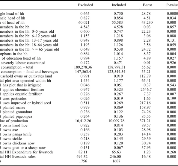
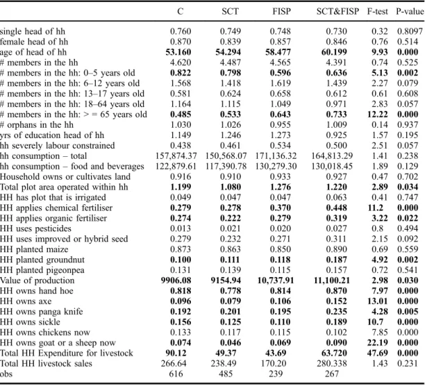
With respect to the original sample, for this paper we selected a subsample in order to identify the stand-alone impact of SCTP and FISP, their synergies, and the joint impact of FISP and SCTP when received jointly. We select 1607 households (interviewed at both baseline and follow-up) that are divided into four groups: control households that neither received SCTP nor FISP (control group); households treated exclusively under SCTP (treatment SCTP); households treatedexclusively under FISP (treatment FISP); and households treated under both programmes simultaneously (treatment SCTP&FISP) (respectively, 38.33, 30.18, 14.87, and 16.6% of the sample). We excluded from the sample the following categories of households: i) included in FISP in both baseline and follow-up (1122); and ii) included in FISP at baseline and in SCTP at follow-up (634).3This kind of selection has advantages and disadvantages. The exclusion of these two groups of households allows us to obtain a clean setting of mutually exclusive groups over which to estimate the impacts of the two programmes in isolation and in combination. However, this selection procedure drastically reduces the sample size (from 3363 to 1607 households interviewed both at baseline and follow-up).4Potentially, it could also affect the randomised nature of the experiment, creating groups with different character-istics at baseline. Indeed, unlike SCTP, access to FISP was not randomised in the evaluation design. In such a case, the identification of the programmes’impact would be biased. In order to deal with this potential sample selection issue, we adopt the doubly robust estimation strategy by Uysal (2015) described inSection 4.1(combination of regression analysis and generalised propensity score weight-ing adjustment).Table B2(in Appendix B in the Supplementary Materials) shows the unweighted tests of differences between the four groups included in the study sample. As suspected, the four groups show significant differences on a variety of baseline household characteristics and economic indicators.

The GPS were estimated through a multinomial logit regression using data at baseline, as in Equation (11).

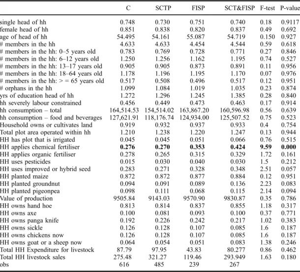
Pr T½ i¼t ¼fðþθXiÞ (11) The variable Pr½Ti¼trepresents the probability of being included in one of the four groups (control, treatment SCTP, treatment FISP, treatment SCTP&FISP). This is modelled as a function of a vector of control variables (Xi) which includes household size and demographic composition, characteristics of the household head, proxies of wealth (total land owned, agricultural assets, and livestock owned), distance to the markets and district fixed effect. The GPS weights allowed to‘rebalance’the sample. Indeed,Table 1 shows that, with only one exception, the four groups are identical at baseline. Equation (12) presents the regression equivalent of difference-in-difference with covariates and weighting based on GPS.

Yi;d ¼ζ þαD2014iþβ1SCTPi;dþβ2ðD2014iSCTPi;dÞ þγ1FISPi;d

þγ2ðD2014iFISPi;dÞ þγ3SCTPi;d FISPi;dþδðD2014iSCTPi;d FISPi;dÞ

þXβXiþμi;d (12)

Table 1. Anova test for difference between groups of intervention: control, SCTP, FISP, SCTP&FISP (adjusted by the Generalized Propensity Score weights)

C SCTP FISP SCT&FISP F-test P-value

single head of hh 0.748 0.730 0.751 0.740 0.18 0.9117 female head of hh 0.851 0.838 0.820 0.837 0.49 0.692 age of head of hh 54.495 54.161 55.087 54.719 0.150 0.927 # members in the hh 4.633 4.633 4.454 4.544 0.59 0.618 # members in the hh: 0–5 years old 0.783 0.769 0.728 0.771 0.27 0.846 # members in the hh: 6–12 years old 1.250 1.256 1.162 1.195 0.74 0.527 # members in the hh: 13–17 years old 0.905 0.905 0.873 0.891 0.11 0.956 # members in the hh: 18–64 years old 1.178 1.196 1.195 1.170 0.07 0.976 # members in the hh: > = 65 years old 0.517 0.508 0.496 0.517 0.12 0.951 # orphans in the hh 1.099 1.084 1.019 1.035 0.23 0.874 yrs of education head of hh 1.272 1.296 1.245 1.385 0.28 0.840 hh severely labour constrained 0.456 0.449 0.473 0.463 0.17 0.914 hh consumption–total 164,514.53 154,514.02 163,867.20 160,596.98 0.56 0.639 hh consumption–food and beverages 127,621.91 118,176.74 124,934.00 125,507.52 0.75 0.523 Household owns or cultivates land 0.919 0.932 0.937 0.933 0.4 0.754 Total plot area operated within hh 1.210 1.238 1.220 1.247 0.13 0.944 HH has plot that is irrigated 0.045 0.045 0.051 0.066 0.76 0.515 HH applies chemical fertiliser 0.276 0.270 0.353 0.424 9.59 0.000

HH applies organic fertiliser 0.278 0.265 0.315 0.329 1.72 0.161 HH uses pesticides 0.015 0.030 0.040 0.030 1.5 0.212 HH uses improved or hybrid seed 0.283 0.271 0.328 0.348 2.51 0.057 HH planted maize 0.872 0.872 0.877 0.884 0.12 0.951 HH planted groundnut 0.094 0.091 0.089 0.136 2.23 0.083 HH planted pigeonpea 0.098 0.111 0.068 0.115 2.14 0.094 Value of production 9505.84 9143.03 9570.90 9830.87 0.35 0.786 HH owns hand hoe 0.813 0.814 0.837 0.855 1.18 0.317 HH owns axe 0.100 0.081 0.093 0.100 0.37 0.771 HH owns panga knife 0.192 0.226 0.242 0.217 1.02 0.383 HH owns sickle 0.126 0.128 0.107 0.085 1.6 0.187 HH owns chickens now 0.126 0.128 0.107 0.085 1.6 0.187 HH owns goat or a sheep now 0.064 0.054 0.051 0.083 1.38 0.246 Total HH Expenditure for livestock 87.79 97.95 43.83 80.277 0.86 0.462 Total HH livestock sales 275.48 321.27 119.46 293.949 1.63 0.180

obs 616 485 239 267

Yi;d is the outcome variables. SCTP and FISP are indicator variables for, respectively, exclusive assignment to either SCTP or FISP. SCTP&FISP is an indicator variable for assignment to both SCTP and FISP.D2014 represents the survey year and is equal to one at follow-up, zero otherwise.

Xis a set of baseline household characteristics (household size and demographic composition, and characteristics of the household head) and controls at community level (a vector of contempora-neous cluster level prices, as well as a set of exogenous shocks and district fixed effects).μ is an error term.

The parameters of interest are the coefficientsβ₂,γ₂andδwhich are, respectively, the treatment effect estimates of SCTP for households treated only by SCTP, the effect of FISP for households treated only by FISP, and the estimate of the joint impact of SCTP and FISP for households treated by both programmes. These parameters allow us to estimate the synergies between the two programmes, as well as their complementarity. In particular, the difference between δ (joint impact of SCTP and FISP when a household receives both),β₂ (stand-alone impact of SCTP) andγ₂ (stand-alone impact of FISP), that is δ-β₂-γ₂, measures the complementarity between the SCTP and FISP. The difference between δandβ₂ measures the incremental impact of FISP on SCTP households. The difference betweenδandγ₂measures the incremental impact of SCTP on FISP households. Note that SCTP, FISP and SCTP&FISP represent mutually exclusive groups. SCTP takes value one if the household is treated exclusively under SCTP, zero otherwise. FISP takes value one if the household is treated exclusively under FISP, zero otherwise. SCTP&FISP takes value one if the household is treated under both SCTP and FISP, zero otherwise (that is neither of the programmes is received, or the household only benefits from one of the programmes). This variable does not represent an interaction between SCTP and FISP. It represents a completely different group of households. For this reason, the stand-alone impacts of SCTP and FISP are, respectively, simply β2 andγ2, and the joint impact of SCTP and FISP isδ. See also Gertler et al. (2011).

Before proceeding to the next section, a challenge related to the analysis of FISP needs to be brought to attention, namely the fact that households treated under FISP may receive different quantities and combinations of maize seed and inorganic fertiliser. Unfortunately from our survey data it is not possible to get an exact measure of subsidised seeds and subsidised fertilisers, but only the equivalent amount in cash of FISP vouchers. Among recipients, there is some variability in the self-reported amounts, which may be due to misreporting or under/over-reporting (Table available upon request). There is likely to be a measurement error, which would complicate a lot of the econometrics, without a clear advantage over the binary approach. In fact, we would need an instrument for the vouchers amount. For this reason we decided to take into account only whether they received FISP or not without taking into account potential differences in the amount of seeds and fertilisers received.

5. Results of the stand-alone and combined impacts of SCTP and FISP

The following sub-sections describe the main findings on a large set of outcomes, including household expenditure, agricultural production and livestock (ownership and expenditure). Findings on the impact on food security and use of agricultural inputs are reported inTables D2andD3in Appendix D in the Supplementary Materials. We present the results for the whole sample and by groups of households with different labour endowments, namely labour constrained and unconstrained. This heterogeneity analysis has not been chosen at random, rather it is justified by the relevance of labour capacity in the targeting mechanisms of both programmes. In our analysis, a household is defined as‘labour constrained’if there is no able-bodied member of the household who is fit-to-work, that is no adult without chronic illness and/or disabilities. All estimates are doubly robust: they include a large set of control variables, namely, baseline head of household’s characteristics, household demographic composition and size, a vector of contem-poraneous cluster level prices, a set of exogenous shocks, and district fixed effect, and are adjusted with the GPS weighting. Confidence intervals consider heteroskedasticity robust standard errors clustered at the community level.

5.1. Consumption expenditure

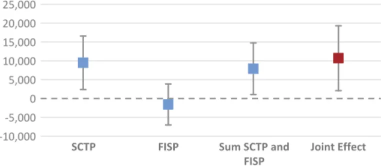
Figure 1provides a graphical representation of the estimated stand-alone impact of SCTP and FISP, their joint impact and their synergies on consumption expenditure per adult equivalent. The thick horizontal bars represent the estimated coefficients, while the thin horizontal bars show the confidence interval. The figure shows, from the left to the right, 1) the alone impact of SCTP, 2) the stand-alone impact of FISP, 3) their sum, and 4) the joint impact of SCTP and FISP when the households benefit from both simultaneously. The difference between 4 and 3 represents the precise measure of complementarity between the two interventions (δ−β2−γ2).

The figure shows that the stand-alone impact of SCTP on expenditure per adult equivalent is positive and significant but the stand-alone impact of FISP is close to zero and not statistically significant. The exclusive receipt of cash transfer leads to an increase of expenditure of 9481 MWK, corresponding to 29 USD (at the exchange rate of 2013). This represents an increase of 21 per cent of the baseline mean value for expenditure. The joint impact is positive and significant (10,697 MWK, equivalent to 32 USD), and it is greater than the sum of the stand-alone impacts of SCTP and FISP. Indeed, the joint impact corresponds to a 24 per cent increase with respect to the baseline mean of expenditure for households receiving both SCTP and FISP. Overall, the estimates for consumption expenditure show positive synergies when households participate in both programmes.

Table 2shows the doubly robust estimates of the incremental impacts of SCTP on FISP and the incremental effect of FISP on SCTP. While the former is positive and statistically significant, corresponding to 12,289 MWK (37 USD), the latter is positive but not significant. This means that the additional impact of cash transfers to households that received exclusively FISP would induce an increase of expenditure per adult equivalent of 37 USD. Moreover, the heterogeneity analysis high-lights strong differences between labour constrained and unconstrained households. Indeed, it shows that the stand-alone impact of SCTP is larger for households defined as labour constrained (a 24% increase relative to baseline mean). However, synergies take place only for households with labour capacity. For this group of households, the incremental impact of SCTP on FISP is positive and significant, equivalent to 20,505 MWK (62 USD) and the complementarity estimate is positive and significant. It shows that the joint receipt of SCTP and FISP induces an increase of expenditure for labour unconstrained households which is 13,412 MWK (40 USD) greater than the sum of the stand-alone impacts of SCTP and FISP. Furthermore, the heterogeneity analysis shows that the baseline mean of expenditure is significantly higher for labour constrained households. This seems to be counterintuitive but is explained by differences in expenditure for food. While labour unconstrained households consume self-produced food, labour constrained households are more likely to purchase from the market. This explanation is supported by the differences in the baseline value of production for labour constrained and unconstrained households, where it is significantly higher for the former group. -10,000 -5,000 0 5,000 10,000 15,000 20,000 25,000

SCTP FISP Sum SCTP and

FISP

Joint Effect

Figure 1. Impact on total expenditure per adult equivalent–MWK real values.

Note: Exchange rate in 2013: 1 USD = 329.4768 MWK.

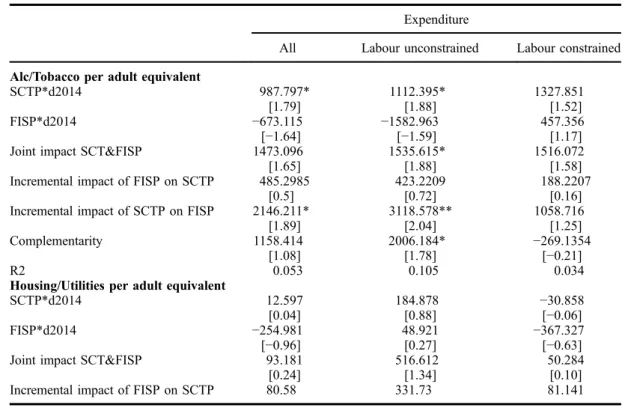
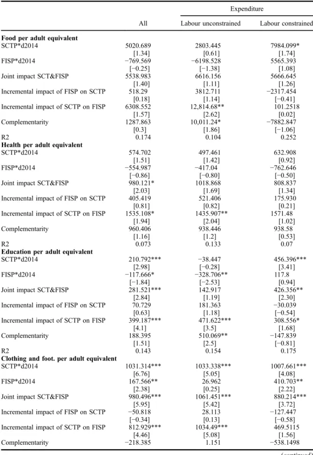
Table 3shows the effect on several expenditure items, namely food, health, education, clothing and footwear (the results for additional expenditure items are reported inTable C2(in Appendix C in the Supplementary Materials). The results for food expenditure are similar to those for total expenditure. Indeed, the stand-alone impact of SCTP is greater for labour constrained households (the coefficient shows an increase of 18% of the baseline per adult equivalent expenditure on food), and the stand-alone impact of FISP is positive but not statistically significant. However, positive synergies occur only for the group of labour unconstrained households. Looking at the estimates of other consumption items, the results are more heterogeneous. In particular, we find synergies between SCTP and FISP for expenditures on health, education and clothing and footwear, but not for the other consumption items. Most of the increase in expenditure is due to SCTP.

Finally, with the exception of expenditure for clothing and footwear, the stand-alone impact of FISP is never positive and significant. This suggests that FISP does not produce an income effect. Indeed, when received alone, it does not release liquidity otherwise used for agricultural inputs such as fertilisers or seeds. This result is consistent with findings of previous studies, both quantitative and qualitative, which document a weak impact of FISP on expenditure (Chirwa & Dorward,2013).

5.2. Agricultural production and livestock

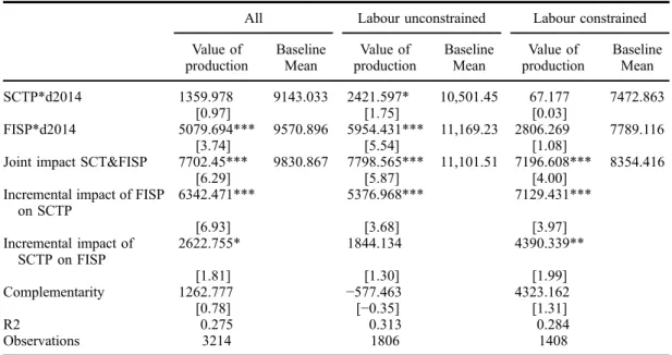
Figure 2provides a graphical representation of the estimated stand-alone impacts of SCTP and FISP, the joint impact and their synergies on value of production. The joint impact is positive and significant and there are positive synergies when households participate in both programmes in increasing the value of production. The figure also shows that most of the increase in the value of production is due to FISP. Indeed, while the stand-alone impact of FISP is large in size, positive and significant (5079 MKW, equivalent to 15 USD, a 53% increase from baseline values), the coefficient of SCTP is small in size and insignificant. Table 4 provides the regression estimates for the value of production,

Table 2. Impact on total expenditure per adult equivalent–MWK real values

All Labour unconstrained Labour constrained

Total expenditure Baseline Mean Total expenditure Baseline Mean Total expenditure Baseline Mean SCTP*d2014 9480.703** 46,207.21 7092.684 38,001.44 13,290.677** 56,296.15 [2.19] [1.37] [2.08] FISP*d2014 −1592.202 50,496.03 −7879.535 45,677.74 6388.564 55,867.32 [−0.48] [−1.62] [1.08]

Joint impact SCT&FISP 10,696.760** 51,667.82 12,625.724* 40,800.66 10,656.982** 64,295.13

[2.04] [1.79] [2.05]

Incremental impact of FISP on SCTP 1216.058 5533.04 −2633.695 [0.32] [1.33] [−0.44] Incremental impact of SCTP on FISP 12,288.96** 20,505.26** 4268.419 [2.24] [3.35] [0.57] Complementarity 2808.26 13,412.58** −9022.259 [0.55] [2.26] [−1.09] R2 0.167 0.129 0.267 Observations 3214 1806 1408

Notes: i)Exchange rate in 2013: 1 USD = 329.4768 MWK.ii)Statistical significance at the 99 per cent (***), 95 per cent (**) and 90 per ent (**) confidence levels. Robust t-statistics clustered at the community level are in brackets. All estimations control for baseline head of household’s characteristics, household demographic com-position and size, a vector of contemporaneous cluster level prices, a set of exogenous shocks, and district fixed effect, and are adjusted with the GPS weighting. Confidence intervals consider heteroskedasticity robust standard errors clustered at the community level.

Table 3.Impact on expenditure per different items–MWK real values Expenditure

All Labour unconstrained Labour constrained

Food per adult equivalent

SCTP*d2014 5020.689 2803.445 7984.099*

[1.34] [0.61] [1.74]

FISP*d2014 −769.569 −6198.528 5565.393

[−0.25] [−1.38] [1.08] Joint impact SCT&FISP 5538.983 6616.156 5666.645

[1.40] [1.11] [1.26]

Incremental impact of FISP on SCTP 518.29 3812.711 −2317.454 [0.18] [1.14] [−0.41] Incremental impact of SCTP on FISP 6308.552 12,814.68** 101.2518

[1.57] [2.62] [0.02]

Complementarity 1287.863 10,011.24* −7882.847

[0.3] [1.86] [−1.06]

R2 0.174 0.104 0.252

Health per adult equivalent

SCTP*d2014 574.702 497.461 632.908

[1.51] [1.42] [0.92]

FISP*d2014 −554.987 −417.04 −762.646

[−0.86] [−0.80] [−0.50] Joint impact SCT&FISP 980.121* 1018.868 808.837

[2.03] [1.69] [1.34]

Incremental impact of FISP on SCTP 405.419 521.406 175.930

[0.81] [0.82] [0.21]

Incremental impact of SCTP on FISP 1535.108* 1435.907** 1571.48

[1.94] [2.04] [1.02]

Complementarity 960.406 938.446 938.58

[1.16] [1.2] [0.53]

R2 0.073 0.133 0.07

Education per adult equivalent

SCTP*d2014 210.792*** −38.447 456.396***

[2.98] [−0.28] [3.41]

FISP*d2014 −117.666* −328.706** 117.8

[−1.84] [−2.53] [0.94] Joint impact SCT&FISP 281.521*** 142.917 426.356**

[2.84] [1.19] [2.30]

Incremental impact of FISP on SCTP 70.729 181.363 −30.039 [0.63] [1.18] [−0.54] Incremental impact of SCTP on FISP 399.187*** 471.622*** 308.556*

[4.1] [3.5] [1.68]

Complementarity 188.395 510.069** −147.839

[1.51] [2.5] [−0.81]

R2 0.143 0.154 0.175

Clothing and foot. per adult equivalent

SCTP*d2014 1031.314*** 1033.338*** 1007.661***

[6.76] [5.05] [4.08]

FISP*d2014 167.566** 26.962 410.703**

[2.38] [0.25] [2.22]

Joint impact SCT&FISP 980.496*** 1061.451*** 880.214***

[5.95] [5.42] [3.72]

Incremental impact of FISP on SCTP −50.818 28.113 −127.447 [−0.34] [0.13] [−0.58] Incremental impact of SCTP on FISP 812.929*** 1034.49*** 469.5115

[4.46] [5.08] [1.56]

Complementarity −218.385 1.151 −538.1498 (continued)

including as an additional regressor the size of cultivated land at baseline. The estimates of the joint impact of the two programmes received simultaneously show a much larger increase of the value of production, which ranges between 70 to 86 per cent of the baseline mean value, for labour

Table 3. (Continued)

Expenditure

All Labour unconstrained Labour constrained [−1.25] [0] [−1.85] R2 0.126 0.157 0.133 Observations 3214 1806 1408 -2,000 0 2,000 4,000 6,000 8,000 10,000 12,000

SCTP FISP Sum SCTP and

FISP

Joint Effect

Figure 2. Impact on value of production–MWK real values.

Note: Exchange rate in 2013: 1 USD = 329.4768 MWK.

Table 4. Impact on value of production–MWK real values

All Labour unconstrained Labour constrained

Value of production Baseline Mean Value of production Baseline Mean Value of production Baseline Mean SCTP*d2014 1359.978 9143.033 2421.597* 10,501.45 67.177 7472.863 [0.97] [1.75] [0.03] FISP*d2014 5079.694*** 9570.896 5954.431*** 11,169.23 2806.269 7789.116 [3.74] [5.54] [1.08]

Joint impact SCT&FISP 7702.45*** 9830.867 7798.565*** 11,101.51 7196.608*** 8354.416

[6.29] [5.87] [4.00]

Incremental impact of FISP on SCTP 6342.471*** 5376.968*** 7129.431*** [6.93] [3.68] [3.97] Incremental impact of SCTP on FISP 2622.755* 1844.134 4390.339** [1.81] [1.30] [1.99] Complementarity 1262.777 −577.463 4323.162 [0.78] [−0.35] [1.31] R2 0.275 0.313 0.284 Observations 3214 1806 1408

Notes: See notesi)andii)inTable 2. These estimates include as an additional regressor the size of cultivated land at baseline.

unconstrained and constrained households. The results show strong synergies between the two interventions since the incremental effect of each programme on the other is positive and statistically significant. Moreover, the heterogeneity analysis suggests that the stand-alone impacts of SCTP and FISP are larger for labour unconstrained households but positive synergies take place more for households defined as labour constrained. Indeed, for labour constrained households the incremental impact of FISP on SCTP is 7129 MWK (22 USD), significantly greater than the same incremental impact for labour unconstrained households (5378 MWK, 16 USD), and the incremental impact of SCTP on FISP is 4390 MWK (13 USD). This is an important result: the combination of a social protection programme and an agricultural development intervention generates more synergies in agricultural production for the most disadvantaged households. We envisaged two potential explana-tions for the stronger synergies on production observed for labour constrained households. They may use part of the additional liquidity for 1) hiring labour and/or 2) purchasing agricultural assets. While the first potential explanation is not supported by our data (see Table C3 in Appendix C in the Supplementary Materials),5the second explanation is upheld by the estimates of the impact of SCTP and FISP on an index of agricultural assets6 (see Table C4 in Appendix C in the Supplementary Materials). Synergies in increasing agricultural assets are stronger for labour constrained households. Table 5shows the results for crop production (land area cultivated for each crop, percentage of households engaged in each crop production, and quantity of crop produced). The exclusive receipt of FISP increases the area of cultivated land for maize for labour constrained households (25% compared to baseline mean) and increases the land cultivated for groundnut for all beneficiary households (23 and 20% of the baseline mean value for labour unconstrained and constrained households, respectively). The evidence of no significant impact on the size of land cultivated for other crops suggests that FISP alone and SCTP and FISP received jointly facilitate the cultivation of land otherwise left unused without FISP and SCTP interventions.7Table 5further shows that FISP positively affects the percentage of households engaged in maize production and also the quantity produced, especially for labour constrained households. For this group, FISP increases the percen-tage of households engaged in maize production by 15 per cent and the quantity of maize produced by 64 per cent compared to the baseline mean. A much larger increase is estimated for production of groundnut (100 and 300% for labour constrained households but such large numbers are due to the extremely low value for participation and quantity produced at baseline). Overall these results are not surprising, since at the time of the data collection, and before the latest reforms, FISP was mainly directed towards enhancing maize production, and only to a minor extent was it also supposed to increase other crops’production, for instance by providing improved seeds for legumes, including groundnuts.

For the quantity of maize produced, the stand-alone impact of SCTP is not statistically significant but the joint effect on participation is significant for the most disadvantaged group of households. For the production of these crops synergies are also taking place. Indeed, the incremental impact of FISP on SCTP on participation of labour constrained households is highly significant. The effect for labour unconstrained household is weak probably because the overwhelming majority of households are already engaged in farming activities (‘ceiling effect’).

As far as the impact on livestock is concerned, inTables 6and 7we looked at whether SCTP and FISP had any impact on ownership of and household expenditure for livestock (chicken and other poultry, sheep or goats, ducks and pigs). Overall the results suggest that the stand-alone impacts of SCTP and FISP are positive and significant, and the two programmes are complementary instruments for investment in livestock. Indeed, SCTP directly affects expenditure for livestock providing immedi-ate cash to beneficiary households. The positive impact of FISP on these expenditures may be due to two reasons: FISP is likely to ease liquidity used for agricultural inputs, and the vouchers provided to FISP-beneficiaries being partially exchanged for cash. The results by labour constraints are striking: the incremental impact of FISP on SCTP, the incremental impact of SCTP on FISP, and the complementarity are stronger for labour constrained households.

T able 5. Impact on production Land cultivated for each crop % HH engaged in: Quantity produced All Labour unconstrained Labour constrained All Labour unconstrained Labour constrained All Labour unconstrained Labour constrained Maize pr oduction SCTP*d2014 0.039 0.037 0.029 − 0.001 − 0.004 − 0.008 18.767 19.641 12.244 [0.50] [0.49] [0.26] [ − 0.03] [ − 0.19] [ − 0.15] [1.22] [1.29] [0.52] FISP*d2014 0.08 − 0.03 0.177* 0.067** 0.014 0.1 12** 65.581*** 61.179*** 61.037*** [1.06] [ − 0.33] [1.78] [2.48] [0.72] [2.52] [6.42] [5.97] [4.49] Joint impact SCT&FISP 0.189*** 0.206** 0.161* 0.033 0.003 0.081 81.418*** 76.181*** 82.667*** [2.79] [2.34] [1.65] [0.98] [0.10] [1.64] [4.32] [3.70] [4.28] Incremental impact of FISP on SCTP 0.15*** 0.17** 0.13* 0.034 0.007 0.089 62.651*** 56.540*** 70.423*** [4.25] [2.62] [1.94] [1.52] [0.28] [2.99] [5.40] [3.29] [4.08] Incremental impact of SCTP on FISP 0.109 0.24** − 0.016 − 0.034 − 0.01 1 − 0.031 15.837 15.002 21.629 [1.5] [2.27] [ − 0.16] [ − 0.94] [ − 0.39] [ − 0.56] [0.78] [0.70] [0.97] Complementarity 0.069 0.20* − 0.045 − 0.033 − 0.007 − 0.023 − 2.93 − 4.639 9.386 [0.82] [1.77] [ − 0.36] [ − 0.94] [ − 0.22] [ − 0.4] [ − 0.19] [ − 0.25] [0.43] R2 0.143 0.109 0.213 0.190 0.089 0.260 0.327 0.322 0.368 Gr oundnut pr oduction SCTP*d2014 0.061* 0.075 0.05 0.090* 0.089 0.088 7.954** 8.654 7.076* [1.84] [1.68] [1.33] [1.86] [1.44] [1.54] [2.23] [1.68] [2.01] FISP*d2014 0.068*** 0.077** 0.064* 0.082*** 0.096** 0.082** 7.861** 6.145 9.508** [3.36] [2.65] [1.94] [4.04] [2.42] [2.37] [2.33] [1.25] [2.16] Joint impact SCT&FISP 0.074** 0.1 15** 0.015 0.105** 0.105* 0.100* 9.038** 9.372** 8.1 12** [2.07] [2.59] [0.38] [2.14] [1.74] [1.99] [2.38] [2.19] [2.21] Incremental impact of FISP on SCTP 0.013 0.040 − 0.035 0.015 0.017 0.012 1.084 0.718 1.035 [0.44] [1.2] [ − 0.84] [0.34] [0.31] [0.19] [0.47] [0.27] [0.24] Incremental impact of SCTP on FISP 0.006 0.038 − 0.050 0.022 0.009 0.018 1.177 3.227 − 1.397 [0.15] [0.81] [ − 0.94] [0.45] [0.14] [0.3] [0.25] [0.60] [ − 0.25] Complementarity − 0.055 − 0.037 − 0.01* − 0.067 − 0.079 − 0.069 − 6.777 − 5.428 − 8.472 [ − 1.5] [ − 0.82] [ − 1.82] [ − 1.43] [ − 1.2] [ − 0.95] [ − 1.63] [ − 0.98] [ − 1.39] R2 0.100 0.137 0.098 0.1 16 0.157 0.103 0.124 0.179 0.103 ₍continued ) Downloaded by [168.202.253.225] at 08:47 16 October 2017

T able 5. ( Continued ) Land cultivated for each crop % HH engaged in: Quantity produced All Labour unconstrained Labour constrained All Labour unconstrained Labour constrained All Labour unconstrained Labour constrained Pigeon pea pr oduction SCTP*d2014 0.003 0.048 − 0.079 0.016 0.102** − 0.109 1.506 2.648 − 0.09 [0.07] [1.02] [ − 1.57] [0.30] [2.05] [ − 1.57] [0.85] [1.25] [ − 0.06] FISP*d2014 0.071* 0.092** 0.029 0.094** 0.095** 0.071 3.706*** 3.916** 3.039** [1.92] [2.23] [0.53] [2.23] [2.33] [1.18] [2.85] [2.43] [2.31] Joint impact SCT&FISP − 0.004 0.01 − 0.032 0.001 0.027 − 0.035 1.929 1.405 2.28 [ − 0.10] [0.13] [ − 0.69] [0.01] [0.49] [ − 0.64] [1.30] [0.82] [1.13] Incremental impact of FISP on SCTP − 0.007 − 0.039 0.047 − 0.015 − 0.074** 0.074 0.424 − 1.243 2.37 [ − 0.34] [ − 0.76] [1.3] [ − 0.86] [ − 2.49] [2.16] [0.41] [ − 0.76] [1.40] Incremental impact of SCTP on FISP − 0.075 − 0.082 − 0.060 − 0.094 − 0.067 − 0.105 − 1.776 − 2.51 1 − 0.759 [ − 1.33] [ − 0.94] [ − 1.02] [ − 1.56] [ − 1.04] [ − 1.58] [ − 0.97] [ − 1.15] [ − 0.34] Complementarity − 0.078* − 0.13* 0.019 − 0.1 10** − 0.169*** 0.004 − 3.282** − 5.159** − 0.669 [ − 1.74] [ − 1.75] [0.28] [ − 2.48] [ − 3.18] [0.05] [ − 2.14] [ − 2.40] [ − 0.32] R2 0.204 0.248 0.196 0.275 0.330 0.266 0.187 0.242 0.157 Nkhwani pr oduction SCTP*d2014 − 0.034 − 0.059 − 0.019 − 0.086* − 0.122* − 0.069 − 0.954 − 2.396 0.366 [ − 1.07] [ − 1.19] [ − 0.54] [ − 1.89] [ − 1.95] [ − 1.52] [ − 0.66] [ − 1.28] [0.25] FISP*d2014 0.012 − 0.032 0.061 0.001 − 0.043 0.06 1.849 0.339 3.651** * [0.33] [ − 0.62] [1.63] [0.03] [ − 0.86] [1.06] [1.45] [0.19] [2.81] Joint impact SCT&FISP − 0.009 − 0.055 0.035 − 0.07 − 0.104 − 0.057 − 0.3 − 2.457 1.856 [ − 0.22] [ − 1.03] [0.87] [ − 1.28] [ − 1.39] [ − 1.36] [ − 0.19] [ − 1.26] [1.19] Incremental impact of FISP on SCTP 0.026 0.004 0.054 0.015 0.018 0.012 0.653 − 0.061 1.489 [1.16] [0.18] [1.34] [0.57] [0.42] [0.38] [0.90] [ − 0.09] [1.14] Incremental impact of SCTP on FISP − 0.021 − 0.024 − 0.026 − 0.072 − 0.061 − 0.1 17* − 2.149 − 2.796 − 1.795 [ − 0.48] [ − 0.47] [ − 0.51] [ − 1.28] [ − 0.86] [ − 1.77] [ − 1.44] [ − 1.53] [ − 0.96] Complementarity 0.01 0.036 − 0.007 0.014 0.061 − 0.048 − 1.195 − 0.399 − 2.162 [0.3] [0.67] [ − 0.13] [0.26] [0.95] [0.69] [ − 0.79] [ − 0.22] [ − 1.16] R2 0.144 0.139 0.198 0.1 15 0.1 12 0.185 0.129 0.1 15 0.192 ₍continued ) Downloaded by [168.202.253.225] at 08:47 16 October 2017

T able 5. ( Continued ) Land cultivated for each crop % HH engaged in: Quantity produced All Labour unconstrained Labour constrained All Labour unconstrained Labour constrained All Labour unconstrained Labour constrained Rice pr oduction SCTP*d2014 − 0.017 − 0.008 − 0.037 − 0.034 − 0.025 − 0.045 − 2.551 − 1.567 − 2.568 [ − 0.66] [ − 0.21] [ − 1.45] [ − 0.80] [ − 0.45] [ − 1.07] [ − 0.86] [ − 0.45] [ − 0.80] FISP*d2014 0.015 0.005 0.015 0.01 0.01 1 0.003 − 0.451 − 1.754 0.294 [0.54] [0.17] [0.57] [0.33] [0.34] [0.08] [ − 0.20] [ − 0.89] [0.13] Joint impact SCT&FISP − 0.018 − 0.031 0.004 − 0.038 − 0.061 0.004 − 4.577 − 5.850* − 1.894 [ − 0.67] [ − 0.97] [0.16] [ − 0.94] [ − 1.22] [0.10] [ − 1.54] [ − 1.91] [ − 0.67] Incremental impact of FISP on SCTP 0.000 − 0.024 0.041* − 0.004 − 0.035 0.049 − 2.026 − 4.283 0.674 [ − 0.01] [ − 0.5] [1.75] [ − 0.1 1] [ − 0.65] [1.32] [ − 0.87] [ − 1.39] [0.34] Incremental impact of SCTP on FISP − 0.032 − 0.036 − 0.01 1 − 0.049 − 0.072 0.001 − 4.126 − 4.096 − 2.188 [ − 0.93] [ − 0.8] [ − 0.36] [ − 1.18] [ − 1.27] [0.02] [ − 1.03] [ − 1.04] [ − 0.61] Complementarity − 0.015 − 0.028 0.025 − 0.015 − 0.047 0.045 − 1.575 − 2.529 0.38 [ − 0.36] [ − 0.53] [0.67] [ − 0.3] [ − 0.75] [0.77] [ − 0.53] [ − 0.77] [0.14] R2 0.102 0.106 0.166 0.102 0.108 0.142 0.077 0.069 0.180 Observations 3214 1806 1408 3214 1806 1408 3214 1806 1408 Notes : See note ii) in T able 2 . Downloaded by [168.202.253.225] at 08:47 16 October 2017

Table 6. Impact on livestock expenses and sales–MWK real values Expenses Sales All Labour unconstrained Labour constrained All Labour unconstrained Labour constrained SCTP*d2014 1172.647*** 1395.706*** 761.950*** −78.668 −44.992 −247.801 [5.95] [6.07] [2.83] [−0.54] [−0.18] [−1.23] FISP*d2014 232.985*** 493.282*** 32.287 57.964 231.508 62.384 [2.96] [3.66] [0.28] [0.37] [0.76] [0.27] Joint impact SCT&FISP 1688.574*** 1478.082*** 1997.143*** 395.800* 383.684 335.607

[5.89] [3.92] [6.19] [1.98] [1.05] [1.06] Incremental impact of FISP on SCTP 515.926* 82.3756 1235.193*** 474.468** 428.676 583.408 [1.82] [0.2] [4.68] [2.03] [1.08] [1.57] Incremental impact of SCTP on FISP 1455.59*** 984.800** 1964.855*** 337.836* 152.176 273.224 [5.04] [2.52] [5.33] [1.7] [0.5] [0.8] Complementarity 282.941 −410.906 1202.906*** 416.505 197.167 521.024 [0.99] [−0.94] [3.83] [1.50] [0.43] [1.17] R2 0.188 0.189 0.271 0.053 0.068 0.132 Observations 3214 1806 1408 3214 1806 1408

Notes: See notesi)andii)inTable 2.

Table 7. Impact on livestock

% HH that own: Quantity

All Labour unconstrained Labour constrained All Labour unconstrained Labour constrained Chicken SCTP*d2014 0.196*** 0.150*** 0.236*** 0.931*** 0.698** 1.365*** [3.81] [2.77] [3.20] [3.03] [2.62] [3.04] FISP*d2014 0.103*** 0.134** 0.029 0.276* 0.408 −0.067 [2.80] [2.29] [0.77] [1.96] [1.34] [−0.31] Joint impact SCT&FISP 0.244*** 0.230*** 0.263** 1.677*** 1.511*** 1.828***

[4.31] [4.54] [2.72] [3.90] [4.19] [3.03] Incremental impact of FISP on SCTP 0.047** 0.080* 0.027 0.746* 0.814** 0.463 [2.32] [1.81] [0.46] [1.90] [2.68] [0.98] Incremental impact of SCTP on FISP 0.141** 0.095 0.234** 1.400*** 1.104** 1.894** [2.56] [1.43] [2.13] [3.29] [2.39] [2.85] Complementarity −0.055 −0.054 −0.002 0.469 0.406 0.529 [−1.35] [−0.71] [−0.03] [1.20] [1.06] [1.08] R2 0.105 0.109 0.149 0.086 0.106 0.140

Goats and sheep

SCTP*d2014 0.108*** 0.114*** 0.075* 0.145 0.263* 0.03 [3.99] [2.99] [1.91] [1.36] [1.84] [0.35] FISP*d2014 0.062* 0.099 0.025 0.145 0.294 0.021 [2.01] [1.53] [0.59] [1.30] [1.46] [0.19] Joint impact SCT&FISP 0.238*** 0.185*** 0.300*** 0.694*** 0.758*** 0.452***

[5.79] [3.75] [5.93] [3.93] [2.99] [4.18] Incremental impact of FISP on SCTP 0.131*** 0.071 0.226*** 0.549** 0.495** 0.422*** [4.31] [1.44] [6.35] [2.96] [2.15] [4.87] (continued) Downloaded by [168.202.253.225] at 08:47 16 October 2017

6. Conclusions and policy implications

This paper contributes to the literature on anti-poverty programme evaluation and to discussions on the design of poverty reduction and smallholder agricultural development strategies by shedding light on the interplay between a social protection intervention and an agricultural programme in Malawi.

Findings from this evaluation challenge important notions underlying the approach to poverty reduction in Malawi: firstly, that poor households should not participate in more than one programme simultaneously since this supposedly represents an inefficient use of resources; secondly, that reducing poverty and vulnerability is the only responsibility of social programmes and that productive inter-ventions should only target the non-poor. The analysis shows that achieving the objectives of FISP and SCTP among poor households is best done by combining these programmes such that a poor house-hold participates in both programmes simultaneously. When combined, there are synergies between SCTP and FISP in increasing expenditure, the value of agricultural production and livestock. Furthermore, the heterogeneity analysis conducted in this paper suggests that synergies between the two programmes are mediated by household labour capacity. On the one hand, we find that the positive synergies between SCTP and FISP in increasing household expenditures are stronger for labour unconstrained households. On the other hand, the synergies in increasing agricultural produc-tion are stronger for labour constrained households.

Compared to previous contributions in the literature focusing on the experience of Malawi, our paper is closely related to Matita and Chirwa (2014) in two ways. Both papers find that SCTP is a more powerful policy intervention for increasing expenditure while FISP is a more effective instru-ment for increasing agricultural production. Moreover, they both find that SCTP is more effective for labour constrained households while FISP for labour unconstrained households. However, our paper

Table 7. (Continued)

% HH that own: Quantity

All Labour unconstrained Labour constrained All Labour unconstrained Labour constrained Incremental impact of SCTP on FISP 0.176*** 0.086 0.276*** 0.549** 0.464* 0.431*** [3.70] [1.24] [4.48] [2.89] [1.73] [3.60] Complementarity 0.069* −0.028 0.201*** 0.404* 0.201 0 .401** [1.71] [−0.34] [3.44] [1.86] [0.68] [2.91] R2 0.129 0.128 0.226 0.083 0.113 0.138

Pigeons, doves or ducks

SCTP*d2014 0.007 0.006 0.001 0.136* 0.263** −0.083 [0.48] [0.37] [0.06] [1.71] [2.33] [−0.83] FISP*d2014 −0.005 −0.006 −0.006 0.065 0.143 −0.045 [−0.38] [−0.27] [−0.34] [1.21] [1.20] [−0.63] Joint impact SCT&FISP 0.060** 0.064* 0.052* 0.280** 0.336** 0.238*

[2.55] [1.84] [1.71] [2.74] [2.09] [1.80] Incremental impact of FISP on SCTP 0.053* 0.058* 0.051 0.144 0.072 0.320* [1.91] [1.7] [1.28] [1.15] [0.45] [1.67] Incremental impact of SCTP on FISP 0.064** 0.070* 0.057* 0.215** 0.192 0.283* [2.65] [1.9] [1.7] [2.12] [1.32] [1.81] Complementarity 0.057* 0.064 0.056 0.079 −0.071 0.365* [1.89] [1.5] [1.31] [0.58] [−0.38] [1.73] R2 0.039 0.044 0.080 0.024 0.031 0.071 Observations 3214 1806 1408 3214 1806 1408

Notes: See noteii)inTable 2.

partially counteracts the results on the synergies between the two programmes with, consequently, different policy recommendations. The simulation conducted by Matita and Chirwa (2014) using nationally representative data suggests that FISP should target households that are moderately poor while SCTP should continue focusing on ultra-poor households. The authors argue that the gains from harmonisation and targeting different households may be greater than delivering these two transfers to the same households. Their rationale is that cash transfers can broaden markets for maize produced through FISP among the moderate poor who produce more than they need. Our study, based on representative data on the lower income quantile of the population of two districts in Malawi, supports a different view: the provision of both SCTP and FISP to the same poor households generates positive synergies, and for some specific outcomes, the joint impact of the two programmes implemented simultaneously is actually significantly greater than the sum of the stand-alone contributions. These findings lead to important considerations related to the target population of programmes; productive agricultural interventions such as FISP have a role to play in reducing poverty and should therefore include ultra-poor households among their target populations, who should also continue participating in social protection programmes such as SCTP.

This raises the question of whether the joint implementation of the two programmes on the same group of households is a cost-effective way to reach the stated goals of SCTP and FISP. In order to provide support to our view, we conducted a‘back of envelop’calculation of the direct benefit-cost ratio of the joint implementation of the programmes. For this exercise, we compared the direct benefits of the joint implementation of the programmes and the cost associated wiyh them. The direct benefits are obtained summing up the estimates of the joint impacts of the programme on total household consumption expenditure (52,936 MWK, corresponding to 161 USD – the full estimates for total household expenditure are reported in Table C1 in Appendix C in the Supplementary Materials) and the value of agricultural production (7702 MWK, corresponding to 23 USD), amounting to a total benefit of 60,638 MKW (184 USD). The total costs are estimated summing up the cost of SCTP transfers (an average of 96 USD per household), obtained from the operational module of the questionnaire, and the cost of FISP (an average cost of 75 USD per household), amounting to a total cost of 171 USD. The benefit-cost ratio calculated comparing the total direct benefits and the total cost is 1.1 USD per 1 USD of combined programme cost, meaning that the benefits derived from the joint implementation of the programmes more than overcome the combined programmes’cost.

To substantiate this result, in a companion paper we conducted a local economy-wide cost-benefit analysis in which we consider not only the direct benefits on the beneficiaries but also the local economy-wide benefits of the project, including spillovers to non-beneficiaries (for details, see, 2017).8Income spillovers to non-beneficiaries are simulated with the use of a Local Economy Wide Impact Evaluation (LEWIE) model. We compare the local-economy benefits, appropriately dis-counted, to the cost of the programmes under three different scenarios (for details, see, 2017): (A) Combined implementation of thestatus quoSCTP and FISP. This scenario envisages a partial

overlapping of SCTP and FISP in ultra-poor and labour constrained households;

(B) Reallocation of resources with non-overlapping targeting, that is SCTP allocated to all ultra-poor households and FISP allocated to non-poor and moderately poor households.

(C) Reallocation of resources with partial overlapping of SCTP and FISP in moderately poor labour constrained households.

The main result of this analysis is that in combination with SCTP, FISP raises the benefit-cost ratio of the SCTP alone. Indeed, in a general equilibrium framework, rising consumption costs due to an increase in demand, and a consequent upward effect on prices, limit the real income benefits from the SCTP alone, but FISP increases the local food supply and lowers food prices. Our analysis shows that the higher benefit-cost ratio is obtained under option A, while the lowest benefit-cost ratio is obtained under option B, respectively 1.97 USD and 1.56 USD per 1 USD of combined programmes’ costs.9

To conclude, the evidence shown here suggests that simultaneously providing agricultural and social protection intervention programmes to poor households can have positive effects in the short-term, which are likely to support poor households in breaking out of the cycle of disadvantage in the medium- and long-term and to prevent the transmission of poverty across generations. The SCTP provides liquidity and certainty for poor households and small family farmers, allowing them to invest in agriculture, and better manage risks. Meanwhile, FISP can also promote growth in the productivity of small family farmers, by addressing structural constraints that limit access to inputs.

Acknowledgments

We thank: Fabio Veras Soares for his peer-review of an earlier version of the article, an anonymous referee and the journal editor for providing essential inputs. We are also grateful for the comments received at the following conferences: the Transfer Project workshop in Addis Ababa, the Centre for the Study of African Economies (CSAE) conference in Oxford, the Pacific Development conference in Riverside, and the fourth Annual Bank Conference on Africa (ABCA) in Berkeley. Errors and omissions are the sole responsibility of the authors. The data used in this paper were collected by the Carolina Population Center at the University of North Carolina (UNC) at Chapel Hill and the Centre for Social Research of the University of Malawi for the impact evaluation of the Social Cash Transfer Programme, commissioned by the United Nations Children’s Fund (UNICEF) in Malawi. The SCTP impact evaluation falls under a larger effort, the Transfer Project, jointly implemented by UNICEF, Food and Agriculture Organization of the United Nations (FAO), Save the Children and UNC, which supports the implementation of cash transfer evaluations in sub-Saharan Africa. The analysis included in this article is part of this broader research agenda. Data are not currently publically available, but the authors will facilitate access to estimation, raw data and code in a timely and effective way, if necessary under license to the ultimate owner.

Disclosure statement

No potential conflict of interest was reported by the authors.

Notes

1. Kilic et al. (2013) explain that the limited pro-poor targeting stems from community-based targeting (that is open forums in which

village residents identify beneficiaries in a collective fashion) that are co-opted by more influential community members. Their analysis suggests that, on average, households that are relatively well-off, connected to community leadership, and residing in agro-ecologically favourable locations are more likely to be FISP beneficiaries and receive more input coupons.

2. For details about the programme implementation and funding, see Asfaw et al. (2015) and Handa et al. (2015b).

3. These groups of households represent, respectively, 33.3 and 18.8 per cent of the original sample.

4. Table B1in Appendix B (available in the Supplementary Materials) provides tests of differences between households

excluded versus households included in the analysis of this paper. The group of households excluded from the study sample is relatively better off. This is not surprising since it includes households that received agricultural input subsidies already at baseline or in the previous two years.

5. Table C3in Appendix C (available in the Supplementary Materials) shows the stand-alone impact of SCTP and FISP, as well

as their joint impact and complementarities on a set of indicators of labour supply (total number of days in farming activities, total number of days in ganyu labour, total number of days in wage labour) and hired labour (days of workers hired, total and by sex). The results show a clear negative and significant impact of the SCTP on hours spent in casual labour (Ganyu labour), especially for labour of unconstrained households. No effect is detected on the number of days in farming activities, number of hours in wage labour and number of days of hired labour.

6. This index is generated through a principal component analysis which includes the following items: hand hoes, axes, panga knifes, sickles, watering cans.

7. To support this view, we regress the total land cultivated for any kind of crop over the same set of regressors included in all the estimates. The results (not included in the paper but available upon request) show that FISP alone and especially FISP combined with SCTP increase the size of total land cultivated. Moreover, the incremental impact of FISP on SCTP is positive and significant for labour constrained households.