Discussion Paper 143
Institute for Empirical Macroeconomics
Federal Reserve Bank of Minneapolis
90 Hennepin Avenue
Minneapolis, Minnesota 55480-0291
December 2005
Optimal Welfare-to-Work Programs
*
Nicola Pavoni
University College London and IFS
Giovanni L. Violante
New York University and CEPR
ABSTRACT __________________________________________________________________________
A Welfare-to-Work (WTW) program is a mix of government expenditures on “passive” (unemployment
insurance, social assistance) and “active” (job search monitoring, training, wage taxes/subsidies) labor
market policies targeted to the unemployed. This paper provides a dynamic principal-agent framework
suitable for analyzing the optimal sequence and duration of the different WTW policies, and the dynamic
pattern of payments along the unemployment spell and of taxes/subsidies upon re-employment. First, we
show that the optimal program endogenously generates an absorbing policy of last resort (that we call
“social assistance”) characterized by a constant lifetime payment and no active participation by the agent.
Second, human capital depreciation is a necessary condition for policy transitions to be part of an optimal
WTW program. Whenever training is not optimally provided, we show that the typical sequence of
poli-cies is quite simple: the program starts with standard unemployment insurance, then switches into
moni-tored search and, finally, into social assistance. Only the presence of an optimal training activity may
generate richer transition patterns. Third, the optimal benefits are generally decreasing or constant during
unemployment, but they must increase after a successful spell of training. In a calibration exercise based
on the U.S. labor market and on the evidence from several evaluation studies, we use our model to
ana-lyze quantitatively the features of the optimal WTW program for the U.S. economy. With respect to the
existing U.S. system, the optimal WTW scheme delivers sizeable welfare gains, by providing more
insur-ance to skilled workers and more incentives to unskilled workers.
_____________________________________________________________________________________
*Pavoni: [email protected]; Violante: [email protected]. We thank Marco Bassetto, Chris Flinn, Narayana Kocherla-kota, Per Krusell, Matthias Messner, Torsten Persson, Chris Pissarides, Rob Shimer, and various seminar partici-pants and discussants for useful comments. Violante thanks the CV Starr Center for research support and the Federal Reserve Bank of Minneapolis for its hospitality. The views expressed herein are those of the authors and not neces-sarily those of the Federal Reserve Bank of Minneapolis or the Federal Reserve System.
1
Introduction
Public expenditures on labor market policies targeted to the unemployed average 3% of GDP, across OECD countries (Martin, 2002). These policies face a delicate trade-off between providing unemployed workers with consumption insurance and re-employment incentives. In order to strike the right balance, governments use a wide range of policy instruments which, broadly speaking, can be divided into “passive” and “active” policies. Two thirds of these expenditures are allocated to passive policies, mainly unemployment insurance and social assistance policies providing income support of last resort once unemployment benefits have expired. The remaining third is allocated to active policies, like job-search monitoring, training, and wage subsidies. Typi-cally, job-search monitoring programs pair the unemployed worker with a public employee (the “caseworker”) who verifies her job-search activity, and often helps with improving interviewing skills and selecting suitable job vacancies. Training programs tend to be one of three types: basic education (brush-up courses for individuals with poor literacy and numerical skills, preparation for high-school level diplomas), vocational training (class-room training in specific occupational skills) and temporary jobs (publicly funded employment in non-profit organizations or government agencies). Interestingly, the share of expenditures on active labor market pro-grams has risen substantially over the past 10 years, and this type of government intervention is now a pivotal ingredient of social welfare policies.
It is instructive to consider how these various policy instruments have been assembled together in the United States and in the United Kingdom. In the United States, since 1935 there exists an unemployment insurance system with vast coverage which replaces on average 60% of the pre-displacement wage. Upon expiration of the unemployment compensation (usually after 26 weeks), other forms of financial support become available. The Temporary Assistance for Needy Families (TANF) program is the most notable example. With the Personal Responsibility and Work Opportunities Reconciliation Act (PRWORA) of 1996, the federal U.S. government limited the payment of TANF benefits to a maximum of 5 years–with tighter limits in several states–and imposed strict participation requirements to active labor market programs for welfare recipients. Broadly speaking, two types of programs have been put in place: “human capital development” programs where the emphasis is on training and skill formation, and “labor force attachment” programs, where the focus is on assistance and monitoring during job search. The Food Stamps program represents the main form of social assistance, once the TANF benefits have expired. Finally, the Earned Income Tax Credit, introduced by the federal government in 1975, represents today the major wage subsidy program for low-income workers (see Moffitt, 2003, for a survey of the U.S. welfare system).
An example of a more structured mix of passive and active policies is the U.K. “New Deal,”a mandatory program for all the unemployed workers introduced in 1998. Formally, the New Deal is organized in four sequential stages. Stage 1 consists of a standard unemployment insurance policy lasting 6 months for younger workers and 2 years for older workers. In stage 2 (the “gateway”), a personal adviser regularly meets with the
worker to assist with and monitor her job search. If after four months the worker is still unemployed, she moves to stage 3 (the “options”) where she enters training for up to one year. At the end of the training program, the worker enters stage 4 (the “follow-through”), another period of job-search assistance/monitoring. Also the U.K. welfare system contains an assistance policy of last resort, called Income Support. Finally, the U.K. system features a large earnings subsidy program for poor households, the Working Family Tax Credit (see Blundell and Meghir, 2001, for an overview of the U.K. system).
It is useful to note, at this point, two common features of the U.K. and the U.S. Welfare-to-Work programs, shared by many other countries as well. First, active policies tend to be implemented after an initial spell of unemployment insurance. Second, policies of pure social assistance (like Food Stamps) are usually ordered last in the sequence of policy interventions.
A Welfare-to-Work (WTW) program is precisely a government expenditure program that combines together passive and active policies, as in the U.S. and the U.K. examples. Clearly, every WTW program implicitly promises a certain level of ex-ante welfare to the unemployed agent. An optimal WTW program is a mix of policies that maximizes the expected discounted utility of the unemployed agent, subject to the constraint of not exceeding a given level of government expenditures. The fundamental trade-off to be solved in the design of an optimal WTW program is the one between offering consumption insurance and eliciting the right effort level in the search or training activity.
The first objective of this paper is to develop a theoretical framework suitable to study the key features of optimal WTW programs. Our point of departure is the classic setup–originated largely from the seminal article of Shavell and Weiss (1979)–where the optimal unemployment insurance contract is studied in the presence of a repeated moral hazard problem: the neutral principal (planner/government) cannot observe the risk-averse unemployed agent’s job search effort (hidden action).1 Following the most recent contributions in the
literature (Wang and Williamson, 1996; Hopenhayn and Nicolini, 1997; Zhao, 2001; Pavoni, 2003a), we build on the seminal insights of Spear and Srivastava (1987) and Abreu, Pearce and Stacchetti (1990) to exploit the recursive representation of the planner’s problem where the expected discounted utility promised by the contract to the unemployed agent becomes a state variable.
We generalize this standard setup in two directions. First, following Pavoni (2003b), we let workers’ wages and their job finding probabilities depend on human capital (skills) and allow human capital to depreciate along the unemployment spell. Human capital is our second key state variable in the recursive representation. Second, we enrich the economic environment of the standard setup with the introduction of a costly monitoring 1Bailey (1978), Flemming (1978) and more recently Fredricksson and Holmlund (2001) and Acemoglu and Shimer
(1999) follow a different approach. They study economies where search effort is observable (i.e., there is no moral hazard) and model unemployment insurance as the optimal policy of a benevolent government that chooses the benefitlevel(not the entire time-path) associated to the welfare-maximizing labor market equilibrium. Recently, Saez (2002) and Laroque (2005) have analyzed the optimality of certain income maintenance programs in the U.S. and France within static models where the worker type is private information.
technology that can be used to observe the worker’s search effort and of a costly skill accumulation technology that can be used to slow down depreciation and, possibly, increase the level of human capital.2
The introduction of human capital depreciation in the problem permits a better representation of labor market data along two important dimensions. First, since wages depend on human capital, in our economy workers experience wage losses upon separation, consistently with the findings of a vast set of empirical studies (Bartel and Borjas, 1981; Ruhm, 1991; Jacobson, LaLonde and Sullivan, 1993; for a survey, see Fallick, 1996). Note that in this literature, unemployment duration is often found to have an independent negative impact on re-employment earnings, beyond job-specific and occupational-specific skill losses (e.g., Addison and Portugal, 1989; Neal, 1995). Second, since we let the job-finding probability depend on human capital, search effort becomes less effective as the unemployment spell progresses, inducing negative duration dependence in the unemployment hazard–a common feature of the data, as reported by Machin and Manning (1999) in their survey. In particular, several studies (e.g., Blank, 1989, for welfare recipients; Bover, Arellano and Bentolila, 2002, for UI benefits recipients) continue finding a rapidly declining hazard even after explicitly controlling for unobserved heterogeneity. Moreover, the existence of human capital depreciation during unemployment represents a potential reason for training policies to be part of an optimal WTW program.3
As discussed earlier, job-search monitoring and training policies are key components of actual WTW schemes. The standard setup (e.g., Hopenhayn and Nicolini, 1997) is unable to address the optimality of such important policy instruments. Enriching the economic environment to include the monitoring and human capital accumulation technologies implies that, along the optimal contract, the planner may find it optimal to make use of them.
The second objective of the paper is to study quantitatively the features of the optimal WTW program for the typical welfare recipient in the U.S. economy and contrast them to the actual welfare system. There is an extended econometric literature on the evaluation of active labor market programs (for surveys, see LaLonde, 1995; Meyer, 1995; Heckman, LaLonde and Smith, 1999; Moffitt, 2003) which provides useful guidance on the effectiveness of different types of interventions, but cannot address the complex question of how to design a government program which combines various instruments and follows the worker throughout her non-employment experience. We use our framework in an attempt to answer this question for the U.S. labor market. We calibrate the parameters of our model to match some key labor market statistics. In so doing, we exploit 2Extending Atkeson and Lucas (1995), Alvarez and Ayiagari (1995) study the optimal level of random monitoring of
agents’ reports on job offers and the long-run stationary distribution of consumption in a pure adverse-selection selection setup with temporary (one-period) job offers, and no human capital dynamics. Recently, Boone et al. (2002) have addressed the issue of the optimality of job-search monitoring within a structural search model of the labor market. They numerically compute the optimal level of monitoring in an economy where every worker is subject to the same monitoring probability. Therefore, they do not fully solve for the optimal contract where the use of each instrument is history-dependent, as we do. Their simpler framework has clearly some other advantages, for example they can study general equilibrium effects which we abstract from.
3Skill depreciation is also a central ingredient in a popular explanation of the comparative unemployment experience
information from the evaluation of several recent U.S. active labor market programs. Next, we solve numerically for the optimal program and, by simulation, derive the optimal sequence of policies, their duration, the pattern of optimal benefits, taxes and subsidies. Finally, we calculate the welfare gains for the worker and the budget savings for the government of shifting from the current scheme to the optimal scheme.
1.1
A Preview of the Main Results
The planner’s recommendations on effort choices and on the use of the costly available (search monitoring and skill accumulations) technologies map naturally into four distinct policy instruments: 1) unemployment insurance, where the planner elicits positive search effort from the agent; 2) job search monitoring, where the planner can observe the search effort upon payment of a cost; 3) training, where the planner pays a cost to slow down human capital depreciation; and 4) social assistance, defined as an income-assistance program of “last resort” with the planner inducing zero search effort and simply insuring the worker. Moreover, as in Hopenhayn and Nicolini (1997), by choosing an agent’s consumption during employment, the planner implicitly sets wage taxes and subsidies.
Our qualitative characterization of the optimal WTW program yields four main results. First, in absence of human capital depreciation, the optimal program does not contemplate switching between policy instruments: the program may select initially different policies for workers with different human capital levels, but each policy is absorbing within the unemployment spell.
Second, with human capital depreciation, when training is not chosen, the typical policy sequence in the optimal WTW program starts from unemployment insurance, switches into job-search monitoring, and then turns into social assistance, which remains the only absorbing policy. The faster the human capital depreciation, the more rapidly the optimal WTW program transits between policy-phases. When the optimal program involves training, the possible policy transitions of the program are richer, so we resort to numerical simulations for a full characterization.
Third, we can entirely describe the dynamics of the government transfers and taxes/subsidies associated to each policy phase of the program. Under social assistance and job-search monitoring, benefits are constant because of full insurance, while due to the presence of the incentive constraint they are decreasing both during unemployment insurance and after an unsuccessful spell of training. After a successful training phase, the optimal benefits must increase.
Fourth, the nature of re-employment wage taxes and/or subsidies is largely determined by competing forces which we explain intuitively. One fairly general result is that, as the optimal program approaches the monitoring phase, earnings subsidies become more and more likely, and during job-search monitoring the subsidy tends to increase with duration. This finding, which is linked to human capital depreciation, contrasts with the
well-known result of Hopenhayn and Nicolini (1997) who uncover that, in an economy without human capital dynamics, taxes should rise with the length of the unemployment spell.
For expositional simplicity, in the benchmark model we make the usual assumption in this literature that the planner fully controls the consumption stream of the agent. This precludes the occurrence of self-insuring trades in the asset market. Recently, several authors have begun to analyze dynamic moral hazard models with hidden savings (Werning, 2002; Kocherlakota, 2003; Shimer and Werning, 2003; Abraham and Pavoni, 2004). In an extension of the benchmark model where the agent can anonymously access a credit market, we show that if the agent faces a no-borrowing constraint, the allocations induced by the same optimal contract can be implemented with the help of one simple additional instrument: a linear, time-invariant interest tax.
When we use our theoretical framework to study the optimality of the current U.S. welfare system, we find that, compared to the existing scheme, the optimal program should feature more job-search monitoring and less basic adult training. This result agrees with a vast empirical evaluation literature that finds adult training (for surveys, see Heckman, LaLonde and Smith, 1999; Heckman and Carneiro, 2002) rather ineffective, with few exceptions. Moreover, we find that the current WTW scheme should provide more insurance for skilled workers and more incentives for unskilled workers.
The size of the welfare gains of switching from the current scheme to the optimal program varies across skill type. High-skill workers who rejoin the employment ranks quickly have small gains, around 1% of lifetime con-sumption; however, low-skill workers with long durations can achieve gains beyond 8% of lifetime consumption. Also budget savings for the government are substantial: the optimal program would reduce public expenditures between 4% and 50%, depending on the worker’s human capital level.
The rest of the paper is organized as follows. Section 2 presents the economic environment (available to the agent in autarky). Section 3 describes the contractual relationship between planner and agent, and presents the recursive formulation of the planner’s problem. Section 4 characterizes the key features of the optimal WTW program. In Section 5 we analyze the implementation of the optimal contract with access to credit markets. Section 6 develops the quantitative analysis applied to the U.S. labor market. Section 7 concludes the paper.
2
The Economy
Preferences: Workers have period utility over consumptionc and effortagiven byu(c)−a. Preferences are
time-separable and the future is discounted at rateβ ∈(0,1). We impose thatc ≥0, and thatu(·) is strictly increasing, strictly concave and smooth, with limc→∞u0(c) = 0. A technical assumption that will prove useful in our characterization is that the first derivative ofu−1is convex. This condition is satisfied by a wide range of
CARA class.4
Employment status and effort: The agent can be either unemployed (z=zu) or employed (z=ze).
During unemployment, she can either search or train–these two activities are mutually exclusive within a period– and search/training effort can be either low or high, i.e.,a∈ {0, e},withe >0. Employment is assumed to be an absorbing state with zero disutility of effort (a= 0).5
Human capital: Workers are endowed with a time-varying stock of human capital (skills)h≥0. During
unemployment, if search or training fails, human capital depreciates geometrically at a constant rateδ∈[0,1]. During employment or after a successful spell of training, human capital accumulates. Letydenote the outcome of the worker activity (search/train) during unemployment, withy ∈ {s, f}, wheresdenotes “success”, andf
denotes “failure”. Then,
hs = Ahα+ (1−δ)h, withα∈[0,1] andA≥0, (1)
hf = (1−δ)h. (2)
Production technology: An employed worker of type hproduces output ω(h). We let ω(·) be a
con-tinuous and increasing function, with ω(h) ∈ [0, ωmax] and ω(0) = 0. During employment, human capital
accumulates through the law of motion (1) at no cost (e.g., through learning-by-doing).
Search technology: During search, both efforta and human capitalhaffect the job finding probability
of an unemployed worker. Denote the unemployment hazard rate asπ(h, a). We assume thatπ(h,0)≡0 and that π(·, e)≡π(·)∈(0,1) is continuous and increasing.
Training technology: The unemployed worker can choose to forego the search option and operate a
training technology to accumulate human capital, upon payment of a cost κT R >0. The training technology requires the unobservable worker’s effort to succeed, but its outcome is stochastic: with probabilityθ(a), where
θ(e)> θ(0) = 0, training is successful, and the worker’s human capital next period accumulates following (1). Upon failure, human capital depreciates according to (2).
Insurance and credit markets: During unemployment the agent is subject to a random event she would
like to (self-) insure against: the outcomey of her search/training activity, which affects both her employment status and her level of human capital, thus her future income. In the baseline model, we study the optimal contract when the worker has no access to storage, insurance or credit markets–in particular we abstract from self-insurance. In Section 5, we will relax this assumption and explore how the same allocations implied by the optimal contract can be implemented when workers have anonymous access to the credit market.
4Newman (1995) highlights the role of the curvature of the first derivative of the cost function for the principal (the
inverse of the agent’s utility function) in a static moral hazard model of entrepreneurship.
It is useful to further discuss some of the assumptions we made in laying out our economic environment. The discrete effort choice is coherent with a long tradition in labor economics and macroeconomics which stresses the importance of fixed costs and the extensive margin in participation decisions (e.g., Cogan, 1981). The assumption that employment is an absorbing state is made, as in Hopenhayn and Nicolini (1997), to focus the analysis of the optimal dynamic contract to the unemployment experience.6 The absence of effort cost and the
presence of learning-by-doing on the job suffice to ensure that the value of employment always dominates the value of remaining unemployed so that no job offer is turned down. These two assumptions have no bearing on the qualitative characterization of the optimal WTW program during unemployment and can be relaxed, as long as employment remains dominant.
The monotonicity ofπinhis a natural property, consistent with the overwhelming evidence that unemploy-ment duration is longer for workers with lower pre-displaceunemploy-ment wage (e.g., Meyer 1990). Strictly speaking, it is a “reduced form” that can be microfounded, for example, in a model where skilled workers have access to wider labor market opportunities, or in a model where productivity on the job is positively correlated with search skills. This monotonicity, together with skill depreciation, induces duration dependence in the unemployment hazard.7
Our specification of πalso displays complementarity between the stock of human capitalhand the search effort levela: increasing effort has a larger impact on the hazard rate the larger the level ofh. Bover, Arellano and Bentolila (Table 4, 2002) document that the receipt of benefits significantly reduces the hazard rate of leaving unemployment and this effect tends to fade away as the unemployment spell progresses (andhdepreciates). It is logical to associate the receipt of benefits with a lower search effort, thus their finding provides a possible foundation for our complementarity assumption.
3
The Contractual Relationship
We now introduce a risk-neutral planner/government (principal) who faces an intertemporal budget constraint with a real interest factor equal toβ−1. At time t = 0, the planner offers the unemployed worker (agent) an
insurance/credit contract that maximizes the expected discounted stream of net revenues (fiscal revenues minus expenditures) and guarantees the agent at least an expected discounted utility levelU0. The value ofU0should
be thought of as an exogenous parameter measuring the “generosity” of the welfare system (e.g., the outcome of voting).
6As long as the layoff rate is exogenous, the qualitative predictions of our model, within the same unemployment spell,
are unchanged. Zhao (2001), and more recently Hopenhayn and Nicolini (2004), introduce a job-separation probability that is under agents’ control and show that the optimal dynamic contract must also take the employment history into account.
7None of our analytical results relies on the strict monotonicity of π inh. For example, in Proposition 6, we will
provide a full analytical characterization of the optimal sequence of policies for the case whereπis constant (and only
Information structure: The planner can perfectly observe the employment statusz,whether the unem-ployed worker is searching or training, and the outcome y of the latter activity.8 However, the agent’s effort
choiceaduring both search and training is private information of the agent, so the planner faces a moral hazard problem.
A search-effort monitoring technology is available to the planner when the worker seeks job opportunities: upon payment of a costκJM >0, the job-search effort of the agent can be perfectly observed and enforced by the planner. The monitoring technology can be interpreted as the situation where the planner pays the services of a “caseworker” who monitors closely the search activity of the agent.9 Such technology is unavailable during
training.10
Contract: In each period t, the contract specifies transfers of resources to the worker, recommendations
on search vs. training activities and on the search/training effort level to exert, and the choice of using the effort-monitoring technology, when search is suggested. The period t components of the contract are contingent on all publicly observable histories up to t and, whenever the monitoring technology is not used, search-effort recommendations must be incentive compatible. The training effort recommendations must always be incentive compatible. Moreover, at everyt, we allow the planner to specify the contract contingent on the publicly observable realization xt ∈ [0,1] of a uniform random variable Xt. We will explain later how this “randomization” may be used in the optimal contract to convexify the planner’s problem and, thus, enhance welfare (see also Phelan and Townsend, 1991; and Phelan and Stacchetti, 2001).
The components of the contract as policies of the Welfare-to-Work (WTW) program: The
combination of unmonitored search, monitored search, use of the training technology, together with the high and low effort recommendations configures six possible options. Notice first that the planner will never choose to pay the monitoring cost and suggest the minimal effort level. The reason is that, sinceπ(h,0) = 0,the observable realization of a successful search activity perfectly detects a deviation from the zero-effort recommendation at no additional cost.11 Moreover, the planner will never choose to pay the training cost and suggest zero effort,
8Since the laws of motion for human capital dynamics are known and deterministic, it is enough knowing the
pre-displacement wage, the occurrence and outcome of training and unemployment duration in order to recover the individual level of human capitalhat every point in the worker’s history.
9Our monitoring technology could be interpreted in a more general way, as “random monitoring”, with one additional
assumption. Suppose that the government observes the agent’s search effort only with some probabilityq < 1.When
u(0) =−∞, then if the government threatens to sanction the shirking worker by not paying any benefit, this random monitoring acts exactly as a perfect monitoring, since the worker will never want to be without consumption for a period. Such monitoring activity will be essentially identical to ours whenever the monitoring cost has a fixed component bounded away from zero.
10While certain elements of the learning effort, such as classroom attendance and homework, are easily verifiable, there
are other key components, like attention, focus and concentration, that are extremely hard to be verified by an external party. It is reasonable to argue that learning is a far more complex activity than job search and, as such, fully monitoring the training effort is not possible.
11Put differently, the incentive-compatibility constraint associated to the zero effort recommendation is a trivial one,
since the planner can punish without limits the worker upon finding a job, an outcome which is off the equilibrium induced by the optimal contract.
sinceθ(0) = 0 and the cost would be wasted. As a result, the planner is left with four options, which we label “policy instruments” of the WTW program, and we index withi.
We denote as “Unemployment Insurance” (i=U I) the joint recommendation of search activity and positive search effort. When positive search effort is suggested together with the use of the monitoring technology, the policy will be labelled “Job-search Monitoring” (i=JM). The zero-effort recommendation in the search activity denotes the “Social Assistance” policy (i=SA). A high-effort recommendation with the use of the training technology describes the “Training” option (i=T R). Finally, during employment, the difference between the wage and the planner’s transfer defines implicitly the employment tax (if positive) or subsidy (if negative).
3.1
Recursive Formulation of the Planner’s Problem
Appendix A describes the sequential formulation of the optimal contract and explains that, following the recursive contracts literature, the contract can be described through a state vector composed by the expected discounted utilityU promised to the agent by the continuation of the contract and the level of human capital
hof the worker.12
Exploiting this recursive representation, consider an unemployed worker who enters the period with state (U, h). At the beginning of the period, the planner selects the optimal policy instrumenti(U, h) by solving
V(U, h) = max
i∈{JM,SA,T R,U I}
Vi(U, h), (3)
where the function V is the upper envelope of the values associated to the different policies. In choosing a particular policy, implicitly, the planner also chooses an effort recommendation a(U, h), the transfer c(U, h),
and the continuation utilitiesUy(U, h) conditional on the outcomeyof the search/training activity. We describe these additional choices in the next section.
As anticipated, the planner in general may decide to use randomizations throughX. In this case, the value function for the planner solves
V(U, h) = Z 1 0 max U(x)∈D V(U(x), h)dx, s.t. : (4) U = Z 1 0 U(x)dx,
whereV(U(x), h) is the upper envelope (3), and the integral constraint in (4) says that the planner is committed to keep his promises, hence he must deliver to the agent continuation utilityU in (ex-ante, with respect to the shockx) expected value terms.
12Strictly speaking, the employment statuszis also a state variable, but since employment is absorbing and presents
no incentive problems, the contract is nontrivial only as long as the worker is unemployed and z = zu.Therefore, in
3.2
The Policies
We now describe in detail the planner problem during employment and during unemployment, under the four policies we considered.
Employment state (wage tax/subsidy): Consider an employed worker with states (U, h). Since
em-ployment is an absorbing state without informational asymmetries, the planner simply solves
W(U, h) = max
c,Us ω(h)−c+βW(U
s, hs)
s.t. : (5)
U = u(c) +βUs,
wherehsis obtained from the law of motion (1). The planner will provide full consumption smoothing for the agent, thus promised utility is constant over time. The promise-keeping constraint implies that in every period the optimal transferce is constant and satisfiesce(U) =u−1((1−β)U). Therefore, the magnitude
τ(U, h) =ω(h)−ce(U) (6) is the implicit tax (or subsidy, if negative) the government imposes on employed workers. State-contingent taxes and subsidies are a key component of an optimal WTW plan.
Unemployment Insurance (UI): When the worker is enrolled by the planner in the unemployment
insurance scheme, the problem of the planner is
VU I(U, h) = max c,Uf,Us−c+β £ π(h)W(Us, hf) + (1−π(h))V(Uf, hf)¤ s.t. : (7) U = u(c)−e+β£π(h)Us+ (1−π(h))Uf¤, U ≥ u(c) +βUf,
where hf is generated through the law of motion (2). The pair ¡Us, Uf¢ are the lifetime utilities promised by the planner contingent on the outcome of search (s denotes success and f failure of the search activity). Given the observability of the employment status, the outcome of search is verifiable. For notational simplicity we have denoted π(h, e) as π(h). The first constraint describes the law of motion of the state variable U
(promise-keeping constraint), and the second constraint states that payments have to be incentive compatible. The expressions forW andV are given by equations (5) and (4), respectively.
the agent is VJM(U, h) = max c,Uf,Us−c−κ JM+β£π(h)W(Us, hf) + (1−π(h))V(Uf, hf)¤ s.t. : (8) U = u(c)−e+β£π(h)Us+ (1−π(h))Uf¤.
Notice the similarity between problem (JM) and problem (U I): the former is identical to (U I) except for the fact that there is no incentive-compatibility constraint in exchange for the additional per period costκJM. This cost can be interpreted as the salary of the government employee (“caseworker”) who monitors and enforces the search activity of the unemployed agent, plus the additional administrative expenditures associated to this task.
Training (TR): The planner can opt to operate the costly stochastic training technology requiring the
unobservable agent’s effort as input. The planner’s problem, when the worker is enrolled in training, is defined as VT R(U, h) = max c,Us,Uf−c−κ T R+β£θV(Us, hs) + (1−θ)V¡Uf, hf¢¤ s.t. : (9) U = u(c)−e+β£θUs+ (1−θ)Uf¤, U ≥ u(c) +βUf,
where we have simplified the notation for the success rate of trainingθ(e) asθ.As usual,¡hs, hf¢are given by (1) and (2).
The first natural interpretation of the training option is formal training. During formal training, workers improve their literacy and/or numerical skills (basic training), or learn some occupational-specific skills (voca-tional training) in the classroom. The costκT R is the per-period/per-head cost of administering the training course, and the probability θ denotes the likelihood of the worker passing the examination or attaining the degree in any given period. The second interpretation is that of atransitional job: the planner paysκT Rto the organization employing the worker for one period and providing her with some job-specific skills. At the end of the period, the worker is still unemployed, but with probabilityθ such on-the-job training was successful and human capital depreciation was contained.
Social Assistance (SA): In social assistance, the worker is “released” by the planner for the current
period, in the sense that the planner does not demand high (search or training) effort, but simply transfers some income to the worker. The problem of the planner is
VSA(U, h) = max
c,Uf −c+βV(U
f, hf)
s.t. :
The expression forV is given by equation (4) and the constraint describes how the promised utilityU can be delivered by a combination of current and future payments.
Below we will prove that if at any point during the contract the planner makes the “zero effort” recommen-dation, it is optimal to do so from that point onward: SAis an absorbing policy. In light of this characterization, it is natural to think ofSAas a pure income-assistance program of last resort.
In what follows, it is convenient to state some basic properties of these value functions. By inspecting problem (5), it is easy to see that the value of employment has the following separable form:
W(U, h) = Ω (h) 1−β −
u−1((1−β)U)
1−β , (10)
where the first term, which can be computed recursively as
Ω (h) = (1−β)ω(h) +βΩ (hs),
is the discounted value of the stream of wages and the second term is the present value of the constant level of benefits guaranteed by the planner to an employed worker. It is easy to see thatW is a continuous function, which is decreasing and concave inU,and increasing inh.
By applying fairly standard results in dynamic programming, one obtains the same continuity, monotonicity and concavity properties for V as well, but two caveats are worth mentioning. First, monotonicity in U is guaranteed whenever at (U, h) the consumption level c associated to the optimal program is positive (e.g., whenever u(0) = −∞). Second, the concavity of V in U is guaranteed because of the randomization in (4). In Appendix B (Proposition 0) we report the proof of all such properties. Finally, the properties of V are inherited by the value functions of each single policy Vi. In particular, all the problems defining policies
i∈ {JM, SA, T R, U I}are also concave.
4
The Optimal WTW Program
We are now ready to study the key characteristics of an optimal WTW program. We begin with a discussion of the economics behind the choice among alternative policies, a useful step to understand two important preliminary results. First, we demonstrate that dynamics in human capital (accumulation and depreciation) are a necessary condition for the optimal WTW program to switch between policies. When an individual’s human capital is constant, the optimal program involves only one policy stage, chosen optimally among JM, UI or SA, and no transition across policies (i.e., each policy is absorbing). Second, we show that even in the presence of human capital dynamics, social assistance maintains its absorbing nature.
We then turn to studying the optimal sequence of policies in the model with human capital dynamics. Here we heavily exploit the recursive formulation of the optimal contracting problem. By projecting the upper enve-lope (3) on the (U, h) state space, we obtain a graphical representation of which policy is optimally implemented
at every (U, h) pair. The state space can then be divided into different connected areas, each corresponding to a specific policy whose value dominates all the others. A key step to this characterization is ranking the slopes of the value functionsVi(U, h) for each policy i with respect to its two arguments. Finally, we describe the dynamics of the government transfers associated to each policy phase of the program.
4.1
Choosing Among Policies: Economic Forces at Work
Within our model, there are several key economic forces that induce the planner to select one particular policy over the other three. For ease of exposition, we divide them into costs and returns. We begin by describing the costs and then move to the returns.
First of all, a planner who wants to implementJM orT Rwill have to incur certain direct expenses associated to the administration of the job search monitoring and training technologies (respectively,κJM andκT R). The larger these costs are, the less attractive these two policies appear compared toU I andSA.
Second, the planner must compensate the agent for her effort. Sinceuis concave, the higher the promised utilityU, the lower the marginal utility of consumption. Hence, the larger the payments of the planner must be to compensate the worker for the fixed disutility of the search/training effort cost e. This “wealth effect” makesSAmore attractive, compared toU I, JM andT R,for high enough levels ofU.
The third cost component is the cost induced by the presence of the incentive compatibility constraint. By using the promise-keeping constraint, the incentive compatibility constraint during unemployment insurance can be conveniently reformulated (independently of the unemployment benefitc), as
Us−Uf ≥ e
βπ(h). (IC1)
The difference between the state-contingent utilitiesUsandUf is increasing ashfalls, through the hazard rate
π(h). Large utility dispersions are associated to large consumption dispersions. Since the agent is risk-averse, in order to compensate her for the wider spread of payments across states, the planner has to deliver a higher average transfer for any given promised utilityU. In sum, incentive costs for the planner (i.e., resource costs of satisfying the incentive-compatibility restriction during U I) increase as human capitalh depreciates. Note that this cost is absent inJM and is independent ofhinT R(because θdoes not depend onh).
Moreover, when the third derivative ofu−1is positive, the cost of providing the utility lottery associated to
(IC1), in terms of consumption payments of the planner, increases withU. Hence, the incentive costs (during bothU I andT R) increase with the level of promised utilityU.13
13To understand this result, consider a static version of our model (hence, abstract fromh). Letg≡u−1and letC i(U)
be the cost for the planner of delivering utilityU under policyi. Then, it is easy to see thatCJM(U) =κJM+g(U+e).
In UI, from the (binding) IC and PK constraints,
We now turn to the returns associated to each optimal policy. Social assistance has no direct returns for the planner. InU I andJM, the returns to search in terms of job finding rate viaπ(h), and earnings once employed viaω(h), are increasing inh. Since from (1)hs increases with h,the returns to human capital accumulation during training are of two types: a higherhraises the effectiveness of future job search in U I andJM and it reduces the future incentive costs duringU I; moreover, it increases earnings upon re-employment.
4.2
The “Absorbing” Nature of Social Assistance
Now, we are ready to state our first result. Consider a situation where, along some history, social assistance turns out to be optimal for the planner. Intuitively, given the absence of IC constraints, during SA the planner offers full insurance to the agent, andU is constant. Because of depreciation, however,hdeclines over time. Ashgets smaller, the incentive cost in U I rises and the returns to search and training fall, hence any other alternative policy becomes less attractive compared to SA, which reinforces the optimality of SA. This mechanism delivers the following result.
Proposition 1 (SA absorbing): SA is an absorbing policy. That is, if it is chosen at any period t,
choosing it thereafter is optimal.
Proof: See Appendix B.
Proposition 1 already establishes one key property of the optimal sequence of policies in a WTW program, as it rules out programs where incentive-provision or monitoring is offered after a spell of social assistance. As discussed in the Introduction, pure income support policies (like Food Stamps in the U.S.) tend to be interventions of last resort, in accordance with our result.
A consequence of Proposition 1 is that, because of its absorbing nature, and sinceπ(h,0) = 0,the equilibrium value ofSA does not depend onhand can be written as
ˆ
VSA(U) =−c
SA(U)
1−β , (11)
wherecSA(U) =u−1((1−β)U) is the constant benefit paid to workers inSA by the planner.
4.3
Human Capital Dynamics Are Necessary for Policy Transitions
In order to study the characteristics of the optimal program in absence of human capital dynamics, we consider the case where human capital is not a state variable (i.e., it remains always constant), thus π(·) and ω(·) do
which implies that the cost isCU I(U) =πcs+ (1−π)cf =πg(U+πe) + (1−π)g(U).
Differentiating with respect toU, we obtain that
CU I0 (U)−CJM0 (U) = h πg0(U+ e π) + (1−π)g 0 (U)i−g0(U+e) which is positive for anyU if and only ifg0is convex (becauseπ(U+e
π) + (1−π)U =U+e). Thus, under this condition,
not depend on hbut π, ω >0. For example, this case occurs when δ =A = 0. The planner’s values of each policy are defined as in Section 3.2, without dependence onh.Since there is no human capital variation, there is no role for training policies.
In the next proposition, we show that the structure of an optimal WTW program in an economy without human capital depreciation is very sharp: each policy is absorbing.
Proposition 2 (No human capital dynamics): If π(·)and ω(·)do not depend on h,every policy (JM,
SA, UI) is absorbing: if policy iis chosen at the beginning of the program, choosing it thereafter is optimal. If, in addition,V is strictly concave, any optimal program must possess such absorbing characteristics.
Proof: See Appendix B.
Consider the problem of a planner facing an agent with initial utility entitlement equal to a levelU0where
only one policy betweenU I, JM andSAis implemented with certainty.14 ForU
0high enough, the search effort
compensation cost is prohibitive and the planner will release the agent immediately into social assistance, which is absorbing.
Suppose now thatU0is such that the planner decides to require the agent to supply positive search effort: the
choice would be between either facing theIC constraint or payingκJM to monitor the agent’s effort perfectly. As the utility entitlement falls, theIC constraint becomes “cheaper” to satisfy, so for low enough initial levels ofU0,the planner will begin by enrolling the agent inU I,while for intermediate values ofU0the planner will
chooseJM as its initial policy. DuringU I,because of incentive compatibility, the state variableU is decreasing which reinforces the optimality ofU I compared to the other available policies, since a smaller U reduces the incentive costs. DuringJM the agent is fully insured: sinceVis concave, keeping the promised utility constant over time and never switching out ofJM is always an optimal policy.
The same logic used in Proposition 2 can be used to rank the slopes of the value function with respect to
U,a result that will be extended in the next section.
Corollary to Proposition 2: The (negative) slopes of the value functions with respect to U satisfy
ˆ
VUSA(U)≥VUJM(U)≥VUU I(U),
where the first inequality holds for any U, whereas the second inequality holds at the crossing point, i.e., at the unique (if any) U where VJM(U) =VU I(U).
Proof: See Appendix B.
14In general at U
0 the optimal program might involve random assignment to different policies in period zero. The
proof of Proposition 2 establishes that, in a stationary economy, period zero is the only period in which such random assignment might occur.
The value of unemployment insurance for the plannerVU I falls more steeply than JM with respect to U because of the incentive cost, and VJM is steeper than ˆVSA because of the effort-compensation cost. These properties imply that the relevant value functions, if they cross, can cross at most once.
4.4
The Optimal WTW Program without Training
In this section we begin the characterization of the optimal WTW scheme in the presence of human capital dynamics. It is useful to start by abstracting from the training option and postpone its introduction to Section 4.5. Our ultimate aim is to answer questions such as: What is the optimal sequence of policies? What are the dynamics of unemployment benefits and taxes/subsidies upon re-employment, within each policy?
The recursive formulation naturally suggests the following two-step strategy to approach these questions. We will first derive a simple graphical representation of the regions within the (U, h) state space where each policy arises as optimal, a result of its own independent interest. Next, by reading the (U, h) state space as a phase diagram–whose dynamics are driven by the policy functionsUy(U, h) describing the law of motion for the endogenous variableU, and by the exogenous laws of motion for human capital (1) and (2)–we will be able to recover the sequence of policies within the optimal WTW program.
Finally, the policy functionsci(U, h) and ce(U), together with the laws of motion for the two states, fully describe the optimal sequence of unemployment benefits, as well as wage taxes/subsidies during the optimal WTW program, sinceτ(U, h) =ω(h)−ce(U).
4.4.1
Representation in the (U,h) Space
In the Corollary to Proposition 2, we have established the relative slopes of the value functions with respect to
U in the stationary case. The next proposition establishes conditions under which the result remains true for the general case with human capital dynamics.
Proposition 3 (Slopes of the value functions with respect to U): Let η(U, h) be the real number
that solves
VU(U, h) =−g0((1−β) (U+η(U, h))),
where g ≡u−1 is the inverse utility function. Assume that η(U, h) is non-increasing in U for every h.Then, the (negative) slopes of the value functions Vi with respect to U satisfy
VU I
U (U, h)≤VUJM(U, h)≤VˆUSA(U) =−g0((1−β)U) for all pairs (U, h).
Proof: See Appendix B.
Given the convexity ofg0, the required condition essentially establishes an upper bound on the curvature of V. For example, in the stationary case with log utility, if the implemented policy isSA thenη(U) = 0, if it is
JM thenη(U) =e/(1−β), and if it isU I then we can establish that η(U) = ¯η > e/(1−β) (Pavoni, 2003a). From the definition ofV, it is therefore easy to see that, in this case, the condition of Proposition 3 is satisfied.
In the next proposition we establish an intuitive ranking on the slope of the value functionsVi across the different policiesi=JM, SA, U I, with respect to human capitalh,under a somehow less restrictive assumption.
Proposition 4 (Slopes of the value functions with respect to h): Assume that the value function
Vis sub-modular and that both V and Vi are differentiable in h.Then, their slopes with respect to hsatisfy
VhU I(U, h)≥VhJM(U, h)≥VˆhSA(U) = 0for all U, h.
Proof: See Appendix B.
The logic of this proposition is that VU I is steeper than VJM because of the incentive cost and VJM is steeper than ˆVSA(invariant toh) because of the returns to search.
To understand the role of submodularity, recall that in the twice-differentiable case submodularity means VU,h(U, h) ≤ 0. The shape of V is generated by two contrasting forces. First, “within-policy” there is a tendency towardsupermodularity: an increase in hraises π(h) and reduces the marginal cost of delivering a given level of utilityU since incentives are more easily provided. However, a highhmakes it more attractive to implement active policies likeJM or U I, and we saw that search-intensive policies have more negative slopes with respect to U. This “between-policy” force that tends to generate submodularity of Vhinges on the fact that the expected flow returnπ(h)ω(h) is an increasing function ofh. The assumption in Proposition 4 holds whenever the second force dominates the first, for example, whenπ(·) is constant and the wage increases with skills, a case that will be analyzed in Proposition 6.15
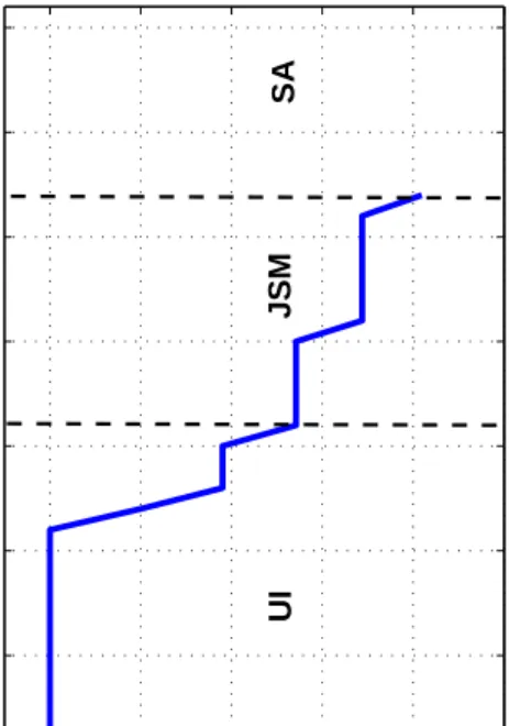
Given our characterization of the relative slopes of Vi with respect toU andh, when the upper envelope
V(U, h) = maxiVi(U, h) is projected onto the (U, h) space, as done in Figure 1, we obtain immediately the regions in the state space where each policy emerges as optimal. Note that these are well defined and connected regions. We start by interpreting Figure 1 as we move “horizontally” in the (U, h) space, i.e., we letU change for a givenh.Next, we study the optimal policies as we move “vertically” through the diagram, i.e., we change
hfor a given level of utility entitlementU.
Moving horizontally (along U): Given any h, start from the highest utility level in the diagram. For
high enoughU, compensating the agent for the high effort is prohibitively costly, and SAis optimal. Moving leftward, as we decrease U the effort compensation cost falls and it becomes optimal to choose a program with high-effort requirement. For intermediate levels ofU, the incentive cost is still high and the value ofJM
15General conditions on the primitives forVto be submodular are hard to establish. One technical reason is that the
nature of themaxoperator is to preservesupermodularity, but not necessarilysubmodularity (e.g., see Hopenhayn and Prescott, 1992).
dominates the value ofU I. As we keep decreasingU,gradually the planner finds it more profitable to face the incentive cost rather than pay the fixed monitoring costκJM, andU I becomes optimal.
Moving vertically (along h): Given anyU, for high levels ofh(i.e., highω(h) andπ(h)), returns from
search are high and incentive costs are low, so U I is optimal. Moving downward, as h falls incentive costs increase and the planner finds it optimal to pay the monitoring cost and implementJM. For very low levels of
h,the returns to search are so low that the planner prefers to save the effort-compensation costs as well, and
SAis the optimal program.
4.4.2
Optimal Sequence of Policies
The optimal sequence of policies is dictated by the evolution of the state vector (U, h). Conditional on unem-ployment,hdeclines monotonically, that is, whenever search is unsuccessful we havehf ≤h. The evolution of
U depends on the specific policy. Formally, we have the following proposition:
Proposition 5 (Optimal Policy Sequence):Assume that Vsatisfies all properties required in
Proposi-tions 3 and 4, and recall that V is a concave function. If V is either strictly concave or strictly submodular or both, then, if at some period t the optimal program selects JM, then next period it is always optimal to either repeat JM or switch to SA. In particular, an optimal WTW program never switches from JM into U I.
Proof: See Appendix B.
It is straightforward to show two properties of the dynamics ofU. First, because of its absorbing nature and full insurance, duringSAthe continuation utilityU is constant. Second, duringU I, the utility entitlementUf promised by the planner to the unemployed worker when search fails tends to decline monotonically to satisfy the incentive constraint.
Third, perhaps surprisingly, during JM the utility entitlement of the agent will increase (see Lemma A7 in Appendix B). There is a simple, almost mechanical, explanation for this behavior. Ashdecreases along the unemployment spell, the optimal program approaches the social assistance option. Because of full insurance, the benefits c are constant between JM and SA, but once in social assistance, the agent will also save the search-effort cost e. Hence, the overall utility is higher inSA, and Uf gradually increases during JM as the implementation ofSA becomes more and more likely in the program.
Combining the dynamics ofhandU with our graphical representation, we immediately obtain another key qualitative characteristic of an optimal WTW program: as soon as the program enters into theJM region, it can either remain inJM or switch toSA.In particular, a transition fromJM toU I is never optimal because both human capital depreciation and the rise in promised utility duringJM worsen the incentive cost and make
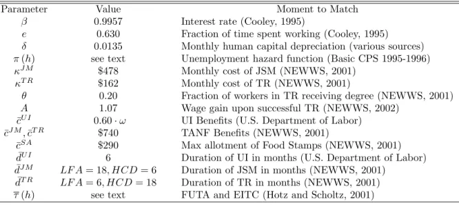
Conditional on failure of search, thetypical sequence of an optimal WTW program without training hence begins with U I followed by JM followed, in turn, by SA. Figure 1 illustrates a simulated individual history of an unemployed worker leading to this optimal sequence of policies.16 Interestingly, this is also the typical
observed sequence of actual programs in many countries: in general, the implementation of active policies starts after a spell of unemployment insurance.
Of course, with the same parameterization, for higher levels of initial promised utility U0 (and/or lower
levels of h0) the optimal program will start in JM and skip U I altogether, and for even higher levels of U0
(and/or even lower levels ofh0) it may start and end withSA. In contrast, for parameterizations where the
monitoring costκJM is especially high,JM may not arise as optimal at all andU I will be directly followed by
SA.
Part of our characterization of the state space and the optimal sequence of policies relies on restrictions on V, which are endogenous.17 Given the discussion following Proposition 4 on the submodularity ofV,it should
be clear that one important special case of the model where such property is satisfied is an economy where the agent is subject only to wage depreciation during unemployment, while the hazard rate functionπ(·) is fixed at some constantπ >0.This important special case is also much easier to handle analytically, and we are able to provide a full characterization of the policy sequence by only imposing conditions on primitives of the model.
Proposition 6 (No duration dependence): Assume that the hazard rate does not change with h and
that it is fixed at π > 0. Then, if at some period t the optimal program selects JM, next period it is always optimal to either repeat JM or switch to SA. In particular, an optimal WTW program never switches from JM into U I.
Proof: See Appendix B.
It may appear surprising, at first, that even though the hazard rate is constant,JM should followU I since we argued that the rise in incentive costs ashdepreciates is associated to the fall inπ(h) and the corresponding widening of the utility spread in (IC1). There is, however, an additional reason why incentive costs go up as
hdepreciates that survives as long asω(·) is increasing in h. In a multiperiod setting, the optimal incentive provision is shaped by the tension between intra- and inter-period consumption smoothing. The planner can improve intra-period consumption insurance (across employment states) by moving part of the punishment burden forward into the future. The emergence ofSA, whereUf cannot decline further, limits the use of the inter-period margin, forcing theU I payments to be biased toward the static component of the incentives. This effective shortening of the time horizon duringU I makes the incentive cost higher for the planner, the lower is
h.
16The parameterization of this example is exactly as in Section 6.1.
17It might be worthwhile mentioning that our numerical simulations have widely verified that the slopes of the value
4.4.3
Optimal Benefits and Wage Taxes/Subsidies
We now turn to the qualitative characterization of the optimal sequence of the unemployment benefits and wage taxes/subsidies. We have the following result:
Proposition 7 (Payments): (i) During unemployment insurance (UI), benefits are decreasing; (ii) during
job search monitoring (JM), the benefits are constant and the wage tax (subsidy) is decreasing (increasing); (iii) during social assistance (SA) benefits are constant; (iv) if π and ω do not depend on h (fixed human capital case), during UI the wage tax is increasing over time, and during JM both the benefits and the wage tax/subsidy are constant.
Proof: See Appendix B.
The need for incentive provision under UI implies that payments should decrease with unemployment duration. Benefits are constant in SA and JM because, within these policies, the absence of incentive problems allows the planner to implement full insurance.
The result on the structure of payments and taxes during UI in the model without human capital dynamics is a re-statement of Hopenhayn and Nicolini (1997) specialized to our environment. A direct consequence of(iv)
is that wage subsidies are either paid at the beginning of the unemployment spell (for particular combinations of highU0 and lowh0), or otherwise they will never be used: the government will never switch from a wage tax
to a wage subsidy during the program. The presence of human capital depreciation changes predictions in two dimensions. First, the behavior of the wage tax duringU I becomes a quantitative issue, which will be discussed below. Second, since the expected gross wageω(h) decreases during unemployment and ceis constant during
JM, the wage taxτ(U, h) =ω(h)−ce(U, h) must now decrease and could become a subsidy.
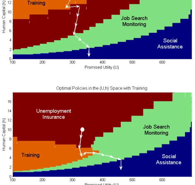
In order to graphically illustrate the key features of the benefits paid across the various policies, it is useful to simulate the model. The bottom right panel of Figure 2 shows the path of wage depreciation. In particular, given the complexity of the algorithm, to reduce the grid points forh, we allow depreciation to be stochastic in the numerical simulations: upon realization of the outcomey=f, human capital either remains constant or falls by one grid point (thehgrid is spaced geometrically). The top left panel shows the behavior of theU I benefits as a fraction of the initial wage, and the net wage (wage minus tax, or plus subsidy) that the unemployed worker would earn if she found a job in that period. The top right panel depicts the implied tax/subsidy, as a fraction of the current wage; the bottom left panel shows the dynamics ofUf which are exactly those depicted on the state space in Figure 1.
As previously discussed, benefits (consumption during unemployment) decrease during U I and remain constant throughout JM and SA because of consumption smoothing. The net wage (consumption during employment) first decreases and then tends to rise asU I approachesJM.There are two main reasons for these