CALCULATION OF COMPOSITE LEADING INDICATORS:
A COMPARISON OF TWO DIFFERENT METHODS
Paper for presentation at the CIRET Conference in
Paris, 10-14 October
by
Olivier Brunet, OECD Secretariat
Keywords: Composite Leading Indicator - Trend Estimation - Phase-Average Trend Method - Data Transformation Detrending Ratio to Trend Normalisation Level Data First Difference Data -Balance Data - Business Tendency Surveys
Olivier Brunet OECD Secretariat
Paris, France [email protected] Session: Macroeconomic Analysis and
CONTENTS
INTRODUCTION... 3
PRESENTATION OF THE INDICATORS... 3
ESTIMATION OF THE TREND: PRESENTATION OF THE TWO METHODS ... 4
PHASE-AVERAGE TREND (PAT)... 4
PERIOD TO PERIOD CHANGES (PPC) ... 5
SMOOTHING ... 5
NORMALISATION: PRESENTATION OF THE TWO METHODS ... 6
NORMALISATION OF PHASE-AVERAGE TREND SERIES (NPT) ... 6
NORMALISATION OF PERIOD TO PERIOD CHANGES SERIES (NPP)... 6
AGGREGATION... 7 LAGGING... 7 WEIGHTING... 7 AGGREGATION... 7 COUNTRY RESULTS ... 8 GERMANY... 8 JAPAN... 10 CONCLUSIONS ... 11 BIBLIOGRAPHY ... 12
Introduction
This study compares the German and the Japanese composite leading indicators using two methods of trend estimation and two methods of data normalisation. These two composite indicators have been selected in order to show that the nature of the component series is important in choosing the calculation method of a composite leading indicator.
The indicator of the first country, Germany, is composed mainly of series from business tendency surveys (qualitative series). For the second country, Japan, the indicator is based mainly on series in level form (quantitative statistical series).
Presentation of the indicators
Sixty-six percent of the German composite leading indicator is composed of business tendency surveys series: Order books: level, Order inflow of flow demand: tendency, Business climate indicator and Finished goods stocks: level. The two other component series are Share prices and Total new orders.
The study is conducted on data from January 1964 to June 2000 in order to compile the composite leading indicator with all data figures available for all component series for the whole period. All series are seasonally adjusted.
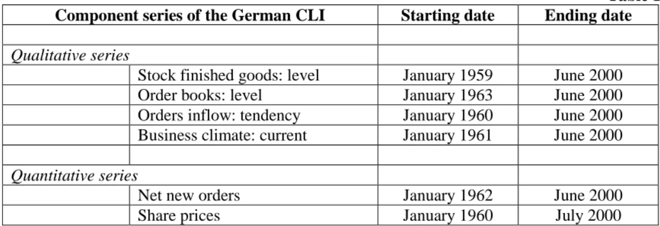
Table 1
Component series of the German CLI Starting date Ending date
Qualitative series
Stock finished goods: level January 1959 June 2000
Order books: level January 1963 June 2000
Orders inflow: tendency January 1960 June 2000
Business climate: current January 1961 June 2000
Quantitative series
Net new orders January 1962 June 2000
Share prices January 1960 July 2000
The German composite leading indicator is very much restricted to components related to activity in the industrial sector of the economy. Out of the six components four refer to industrial activity as
measured by the business survey in industry. The remaining two components refer to a volume series on new orders and the share price index.
The Japanese composite leading indicator only contains of two business tendency surveys series: Finished goods stocks: level and Business situation: prospects. The rest of the series (77%) are series in level form and include: Producer inventory ratio to shipment, Excess of imports over exports, Total stocks in manufacturing, New loans for equipment (commercial banks), Ratio loans to deposits, Share prices Tokyo stock exchange and New vacancies.
The study is conducted from January 1974 to April 2000 in order to compile the composite leading indicator with all data available for all component series for the whole period. From April 1998, the Japanese composite leading indicator is only calculated using eight components because the series New loans for equipment is only available until March 1998. All series are seasonally adjusted.
Table 2
Component series of the Japanese CLI Starting date Ending date
Qualitative series
Business climate: future tendency 2nd Quarter 1967 2nd Quarter 2000 Stock finished goods: level 1st Quarter 1963 2nd Quarter 2000
Quantitative series
Inventory shipment ratio January 1955 May 2000
Total stocks in manufacturing January 1955 April 2000
New vacancies January 1957 June 2000
Share prices January 1959 June 2000
New loans for equipment January 1955 March 1998
Ratio loans to deposits January 1955 May 2000
Excess of imports over exports January 1973 June 2000
Estimation of the trend: presentation of the two methods
Phase-Average Trend (PAT)
This first method estimates a trend in a direct way and removes it from the series. For the trend estimation, we use the Phase-Average Trend method.
The first consideration in the construction of a composite cyclical indicator is that of amplitude-stationarity. The first objective is to ensure that each individual indicator series included in the composite indicator is stationary in some way. The "growth cycle" or "deviation-from-trend" approach is used. Trend estimation is thus a crucial step in detecting cyclical movements and identifying turning points.
The PAT method requires an initial list of turning points, which define the cyclical phases, in order to estimate a trend which cuts through the phases. A first list of turning points is obtained from the preliminary peaks and troughs identified by calculating a first trend estimate based on a 75-month moving-average. A series of tests are then executed on the deviations from the trend in order to eliminate extreme values; and to specify a minimum duration of each phase (5 months) and the minimum duration of each cycle (15 months). The final trend is then calculated with a validated list of turning points as input to the PAT program. The detrended results (deviations from long-term trend) are then used as input to the composite calculation.
Period to Period Changes (PPC)
This second method removes the trend by transformation of data to stationary form by applying the period to period changes to data. This method has been applied to all quantitative series:
2 ) ( 1 1 − − + − = t t t t t X X X X S
with: S : Period to period changes series X : Quantitative series
t : Time
Concerning the qualitative tendency business survey series, it is not necessary to apply the period to period changes or first difference method to this kind of series because data are first differences by nature. For business tendency surveys series, data fluctuate over a level which is a constant figure and therefore series do not have a trend. The balance i.e. the difference between positive and negative answers is used for the business tendency survey series.
Smoothing
Before the normalisation stage, we need to smooth both the quantitative series and the period to period change series. The method of smoothing is explained as follows:
It is necessary to ensure that all component series have equal “smoothness”. This is to ensure that period-to-period changes in the composite indicator are not unduly influenced by irregular movements in any one indicator series. The "Months for Cyclical Dominance" (MCD) moving average is used. This procedure ensures approximately equal smoothness between series and also ensures that the period-to-period changes in each series are more likely to be due to cyclical than to irregular movements. The data lost at the end of the series due to the moving average are restored with an extrapolation by regression over the end of the series.
The MCD values for most series across investigated countries are in the range 1-3. A MCD value of 1 means that no smoothing is needed and this concerns only a few components: for Germany: Order books: level with exception of Order inflow: tendency, and for Japan: Business climate, Finished goods stocks: level and Total stocks in manufacturing. Most financial and other business survey indicators have an MCD of 2 or 3 while most quantitative statistical indicators show MCD values of 4, 5 or 6 such as Excess of imports over exports and Loans for equipment for Japan. The smoothing performed on the component series ensures that the composite leading indicators across all countries are smooth with a MCD value of 1, which means that no further smoothing is needed for an easy identification of a cyclical turning point.
In the following table, the MCD moving average results with the two different methods are presented for all series. The column “transformation” indicates whether the series has been transformed to period to period change series. The transformation has been made only for the quantitative series and the results show how the irregular component has increased for the change series which now have MCD moving average of 6.
Table 3
Japan MCD (PAT) Transformation MCD (PPC)
Business climate: future tendency 1 No 1
Stock finished goods: level 1 No 1
Inventory shipment ratio 2 Yes 6
Total stocks in manufacturing 1 Yes 6
New vacancies 3 Yes 6
Share prices 2 Yes 6
New loans for equipment 4 Yes 6
Ratio loans to deposits 2 Yes 6
Excess of imports over exports 6 Yes 6
Germany MCD (PAT) Transformation MCD (PPC)
Stock finished goods: level 2 No 2
Order books: level 1 No 1
Orders inflow: tendency 5 No 5
Business climate: current 2 No 1
Net new orders 3 Yes 6
Share prices 2 Yes 6
Normalisation: presentation of the two methods
Normalisation or standardisation of component series is necessary in order to minimise the influence of series with marked cyclical amplitude on the composite indicator.
Normalisation of Phase-average Trend series (NPT)
In this first method normalisation is performed on detrended series and involves two steps, first the mean of the MCD moving average series is subtracted to the MCD moving average series itself. Then this series is divided by the mean of the absolute values of the differences of the MCD moving average series from its mean. The normalised series are then converted into index form by adding 100. This method standardizes the amplitudes of the cyclical movements but leaves the relative magnitudes of the irregular movements unchanged. We are going to apply this method to the method PAT. In the rest of the paper, the composite leading indicator compiled by the methods PAT then NPT is called the First method.
Normalisation of Period to Period changes series (NPP)
This second method normalisation is performed on the period to period change series and qualitative business tendency survey series. For period to period changes series, it is carried out by dividing the series by the mean of the absolute values of the period to period change data. For the business tendency surveys series, period to period changes method is not applied. Therefore, normalisation is performed by dividing the series by the mean of the absolute values of the qualitative series. The MCD moving average method (see part ??) is then applied to each component series (qualitative series and period to period changes series) in order to get a smoothed series. We are going to apply this method to the method PPC. In the rest of the paper, the composite leading indicator compiled by the methods PPC then NPP is called Second method.
We tried to apply the MCD moving average method directly to the aggregated composite leading indicators issued from the second method but the results were very difficult to interpret due to the
irregularity of the composite series. Applying the MCD to each series really gives better results for interpretation.
Aggregation
The aggregation method (in order to calculate the composite leading indicators) contains three steps: lagging, weighting and then aggregation.
Lagging
It may sometimes be necessary to lead or lag particular indicators. In this study, no lagging is undertaken.
Weighting
Different weights may be assigned to component series in order to reflect their economic significance (coverage and economic reason), statistical adequacy, cyclical conformity, speed of availability of data, etc. The purpose of weighting is to improve reliability by giving higher weight to components with good quality i.e. indicators which correlate highly with each other and the resultant composite indicator.
In this study, equal weights are used to obtain each country's composite leading indicator. Equal weighting implies, by default, a judgement on appropriate weights, and the normalisation process is itself a weighting system in reverse.
Aggregation
In this study, the raw composite index is obtained by averaging the normalised indices of each component series. A composite index calculated on an incomplete set of data is linked to the body of the index by use of a linking factor which is equivalent to applying the growth-rate of the "incomplete" index to the last point at which a full index is available. For the German (January 1964) and Japanese (January 1974) composite leading indicator, beginning dates are the same for all component series.
For Japan and Germany, two composite leading indicators by country are compiled with the two different methods described. The following section presents the graphical and empirical results of the study:
Country results
Germany
Chart 1 shows the industrial production and the German composite leading indicator (ratio to trend series) compiled with the first method.
Chart 1
Chart 2 shows the industrial production and the German composite leading indicator (ratio to trend series) compiled with the second method.
Chart 2
A comparison of the two leading indicators shows that the patterns are quite similar except for a brief period between 1988 and 1990.
In d u s t ria l p ro d u c t io n a n d C o m p o s it e le a d in g in d ic a t o r S e c o n d m e th o d 8 5 9 0 9 5 1 0 0 1 0 5 1 1 0
Jan-64 Jan-66 Jan-68 Jan-70 Jan-72 Jan-74 Jan-76 Jan-78 Jan-80 Jan-82 Jan-84 Jan-86 Jan-88 Jan-90 Jan-92 Jan-94 Jan-96 Jan-98 Jan-00 In d u s tr ia l p r o d u c tio n Co m p o s ite le a d in g in d ic a to r In d u s t ria l p ro d u c t io n a n d C o m p o s it e le a d in g in d ic a t o r F i r st m e th o d 8 5 9 0 9 5 1 0 0 1 0 5 1 1 0
Jan-64 Jan-66 Jan-68 Jan-70 Jan-72 Jan-74 Jan-76 Jan-78 Jan-80 Jan-82 Jan-84 Jan-86 Jan-88 Jan-90 Jan-92 Jan-94 Jan-96 Jan-98 Jan-00 In d u s tr ia l p r o d u c tio n C o m p o s ite le a d in g in d ic a to r
In table 4, three composite leading indicators are presented and the study is conducted over the period 1963-1999. The first is the OECD composite leading indicator compiled with fixed turning points and the second is calculated with automatically selected turning points. These two composite leading indicators are compiled with the first method. The third one is compiled with the second method.
Table 4
Performance 1963-1999
Against ratio to trend of industrial production
Turning point analysis Cross-correlation
Median lead (+) in months at
Germany
Composite Indicator MCD Peak Trough
All turning points Mean absolute deviation around median Months Lag (+) Peak value
OECD (fixed turning points)
Composite Leading Indicator : OECD method
1 5.5 5 5 6.0 8 0.75
Automatic turning points
Composite Leading Indicator : First method
1 6 2 3 6.2 5 0.74
Composite Leading Indicator: Second method
2 9 5 6 7.7 8 0.54
The composite leading indicator compiled with the first method and automatic turning points has a lead of five months against the industrial production whereas the composite leading indicator compiled by the OECD shows a lead of eight months. The only difference between these two indicators is the method of determination of the turning points which points in favour of the OECD method. On the other hand, the composite leading indicator compiled with the second method shows almost the same good results as the OECD one except that the MCD equals 2. This value of MCD is due to the two quantitative series.
The second method improves the lead at turning points and in particular at peaks. But the cross correlation result is quite low (0.54). The first method does not bring any improvements to the two other ones for the criteria shown in table 4. In addition, the lead that gives the best cross-correlation is
Japan
Chart 3 shows the industrial production and the Japanese composite leading indicator (ratio to trend series) compiled with the first method.
Chart 3
Chart 4 shows the industrial production and the Japanese composite leading indicator (ratio to trend series) compiled with the second method.
Chart 4
For Japan, unlike the composite leading indicator for Germany, the differences between the two methods are significant. The second method gives a more irregular composite leading indicator and does not define troughs as well as the first method.
In d u s t ria l p ro d u c t io n a n d C o m p o s it e le a d in g in d ic a t o r F i r st m e th o d 8 0 9 0 1 0 0 1 1 0 1 2 0
Jan-74 Jan-76 Jan-78 Jan-80 Jan-82 Jan-84 Jan-86 Jan-88 Jan-90 Jan-92 Jan-94 Jan-96 Jan-98 Jan-00 In d u s tr ia l p r o d u c tio n C o m p o s ite le a d in g in d ic a to r In d u s t ria l p ro d u c t io n a n d C o m p o s it e le a d in g in d ic a t o r S e c o n d m e th o d 8 0 9 0 1 0 0 1 1 0 1 2 0
Jan-74 Jan-76 Jan-78 Jan-80 Jan-82 Jan-84 Jan-86 Jan-88 Jan-90 Jan-92 Jan-94 Jan-96 Jan-98 Jan-00 In d u s tr ia l p r o d u c tio n Co mp o s ite le a d in g in d ic a to r
Table 5
Performance 1974-1999
Against ratio to trend of industrial production
Turning point analysis Cross-correlation
Median lead (+) in months at
Japan
Composite Indicator MCD Peak Trough
All turning points Mean absolute deviation around median Months Lag (+) Peak value
OECD (fixed turning points)
Composite Leading Indicator : OECD method
1 6 4 5 3.8 6 0.81
Automatic turning points
Composite Leading Indicator : First method
1 9 4.5 6 4.7 4 0.77
Composite Leading Indicator: Second method
3 12 0 2 8.2 5 0.47
First of all, the results given by the second method are bad compared to the two other methods. Indeed, the composite leading indicator calculated using the second method is quite irregular (MCD equals 3). The high MCD value is explained by the fact that seven of the nine turning points are quantitative series with MCD equals 6. The cross-correlation is low (0.47) and the median lead to trough is 0.
On the other hand, the first method improves the forecast ability at turning points, especially at peaks (9 months against 6 months for OECD method) without improving too much the deviation around median. At the same time, the cross-correlation is slightly lower (at 77% for a four months lead).
Conclusions
This paper has examined the use of two different calculation methods for two countries, Germany and Japan, which each have different types of components series. The German composite leading indicator is mainly composed of business tendency survey series while the Japanese composite leading indicator mainly has quantitative series. The main conclusions are:
- The second method (normalised period to period changes) generates a rather irregular composite indicator with MCD of 2 or 3. This makes it difficult to identify promptly coming turning points. This behaviour is related to the type of component series used and the need for transformation to stationary series. The second method works well with qualitative business tendency survey series where no transformation is used.
- With fixed turning points, the first method (normalised PAT) seems to be the better method to compile a composite leading indicator whatever the set of components (quantitative or qualitative).
- However, trend estimation as used in the first method is more difficult to perform and revisions at the end of the series may change the trend slightly. This will however in general not change the dating of turning points.
Overall, this paper shows that choice of calculation method depends on the nature of the component series.
Bibliography
OECD, “OECD Leading Indicators and Business Cycles in Member Countries, Sources and Methods 1960-1985”, No.39 January 1987;
OECD, “OECD Leading Indicators”, Ronny Nilsson, Economic Studies, No. 9, Autumn 1987; OECD, “Leading Indicators for OECD, Central and Eastern European Countries”, Ronny Nilsson, Article published in the book “Is the Economic Cycle Still Alive?”, edited by Baldassarri/Annunziato, St Martins Press Inc., New York 1994/The Macmillan Press LTD, London 1994;
OECD, “Cyclical Indicators and Business Tendency surveys”, OCDE/GD(97)58, General Distribution; 1997;
OECD, “An update of OECD Leading Indicators”, Gérald Petit, Gérard Salou, Pierre Beziz and Christophe Degain, Paper presented at the OECD Meeting on Leading Indicators, Paris October 1996; OECD, “The 1994 Mexican Crises: Were Signals Inadequate?“, Pierre Beziz and Gerald Petit, Paper published in the Cambridge Review of International Affairs (Summer/Fall 1997);
OECD, “Procedures for constructing composite indexes: a re-assessment”, J. Cullity and A. Banerji, Paper presented at the OECD Meeting on Leading Indicators, Paris October 1996;
OECD, “Confidence indicator and composite indicator”, Ronny Nilsson, Paper presented at the 25th
CIRET conference, Paris October 2000.
OECD, “The OECD System of Leading Indicators: Recent Efforts to Meet User’s Needs”, Benoit Arnaud, Paper presented at the 25thCIRET conference, Paris October 2000;
National Bureau of Economic Research (NBER), “Programmed turning Point Determination”, Gerhard Bry and Charlotte Boschan, Paper published in Cyclical Analysis of Time Series: Selected Procedures