2016
Three essays on multi-level optimization models
and applications
Mohammad Rahdar
Iowa State UniversityFollow this and additional works at:
https://lib.dr.iastate.edu/etd
Part of the
Industrial Engineering Commons
, and the
Operational Research Commons
This Dissertation is brought to you for free and open access by the Iowa State University Capstones, Theses and Dissertations at Iowa State University Digital Repository. It has been accepted for inclusion in Graduate Theses and Dissertations by an authorized administrator of Iowa State University Digital Repository. For more information, please [email protected].
Recommended Citation
Rahdar, Mohammad, "Three essays on multi-level optimization models and applications" (2016).Graduate Theses and Dissertations. 15795.
by
Mohammad Rahdar
A dissertation submitted to the graduate faculty in partial fulfillment of the requirements for the degree of
DOCTOR OF PHILOSOPHY
Major: Industrial Engineering
Program of Study Committee: Lizhi Wang, Co-major Professor Guiping Hu, Co-major Professor
Caroline Krejci Sarah M Ryan
Zhijun Wu
Iowa State University Ames, Iowa
2016
DEDICATION
I would like to dedicate this dissertation to the memory of my late father, who I have not seen him for more than twenty years, but never forgotten. To my mother for her ongoing love and support and to my brother for his words of inspiration and encouragement.
TABLE OF CONTENTS
LIST OF TABLES . . . v
LIST OF FIGURES . . . vi
ACKNOWLEDGEMENTS . . . viii
ABSTRACT . . . ix
CHAPTER 1. GENERAL INTRODUCTION . . . 1
BIBLIOGRAPHY . . . 7
CHAPTER 2. POTENTIAL COMPETITION FOR BIOMASS BETWEEN BIOPOWER AND BIOFUEL UNDER RPS AND RFS2 . . . 10
Abstract . . . 10 2.1 Introduction . . . 10 2.2 Model . . . 14 2.3 Results . . . 18 2.4 Conclusions . . . 30 2.5 Appendix A . . . 32 2.6 Appendix B . . . 34 BIBLIOGRAPHY . . . 37
CHAPTER 3. A TRI-LEVEL OPTIMIZATION MODEL FOR INVEN-TORY CONTROL WITH UNCERTAIN DEMAND AND LEAD TIME . 40 Abstract . . . 40
3.1 Introduction . . . 40
3.2 Model formulation . . . 42
3.2.1 Problem statement . . . 42
3.2.3 Tri-level optimization model . . . 45 3.3 Algorithm design . . . 48 3.4 Numerical results . . . 50 3.4.1 Simulation setup . . . 51 3.4.2 Simulation results . . . 52 3.5 Conclusions . . . 56 BIBLIOGRAPHY . . . 59
CHAPTER 4. A NEW BRANCH AND BOUND ALGORITHM FOR THE BILEVEL LINEAR PROGRAMMING PROBLEM . . . 62
Abstract . . . 62
4.1 Introduction . . . 62
4.1.1 Definitions . . . 63
4.1.2 Categorizing BLP into seven different cases . . . 64
4.2 Literature review . . . 69
4.2.1 Branch and Bound . . . 70
4.2.2 Big-M method . . . 72
4.2.3 Benders algorithm . . . 73
4.3 The new branch and bound algorithm . . . 75
4.3.1 An alternative objective function for the problemD(v) . . . 80
4.4 Numerical results . . . 82
4.5 Conclusions . . . 84
BIBLIOGRAPHY . . . 86
LIST OF TABLES
Table 2.1 Modeling results in four cases . . . 19
Table 3.1 Notation in the deterministic model . . . 44
Table 3.2 Notation in the tri-level model . . . 46
Table 3.3 Simulation data . . . 52
Table 3.4 Average order, inventory level, and shortage in each period for one ex-ample and all models . . . 57
Table 4.1 Seven possible types of BLP problem . . . 68
Table 4.2 The solution of nodes by implementing the new algorithm . . . 81
Table 4.3 Average computation times (in seconds) for ten groups of BLP instances. 83 Table 4.4 Average number of iterations for ten groups of BLP instances. . . 84
LIST OF FIGURES
Figure 2.1 The U.S. renewable energy portfolio in 2012. Data from AEO (2012) . 11
Figure 2.2 Modeling structure . . . 16
Figure 2.3 Projection of biomass based renewable energy consumption in the U.S. Results from our model are combined with data from AEO (2012). . . 20
Figure 2.4 Projection of renewable energy consumption in the U.S. from Table A17 in AEO (2012) for the reference case . . . 21
Figure 2.5 Projection of renewable energy consumption in the U.S. from our model under the base case scenario combined with partial data from AEO (2012). 22 Figure 2.6 Wind power generation in top 20 states between 2013 and 2035. . . 22
Figure 2.7 Geothermal power generation in top 10 states between 2013 and 2035. 23 Figure 2.8 Solar power generation in top 20 states between 2013 and 2035. . . 23
Figure 2.9 Biopower generation in top 10 states between 2013 and 2035. . . 23
Figure 2.10 Cellulosic biofuel production in top 20 states between 2013 and 2035. . 24
Figure 2.11 Renewable energy portfolios in top 30 states broken into four types of resources averaged between 2013 and 2035, excluding biomass for non-cellulosic biofuel production. . . 24
Figure 2.12 Sensitivity of total renewable electricity generation. . . 27
Figure 2.13 Sensitivity of wind power generation. . . 28
Figure 2.14 Sensitivity of geothermal power generation. . . 28
Figure 2.15 Sensitivity of solar power generation. . . 29
Figure 2.16 Sensitivity of biopower generation. . . 29
Figure 2.17 Sensitivity of cellulosic biofuel production. . . 30
Figure 3.1 Rolling planning horizon approach . . . 43
Figure 3.3 The sample probability distribution of the total costs for tri-level and three deterministic models with different holding and shortage costs . . 54
Figure 3.4 Impacts of holding and shortage costs on the relative performance ratio of the total cost . . . 55
Figure 3.5 Impacts of holding and shortage costs on the fill-rate . . . 55
Figure 3.6 The average costs per period of four models and nine cases for one example 57
Figure 4.1 Diagram of the new branch and bound algorithm . . . 78
ACKNOWLEDGEMENTS
I would like to express the deepest appreciation to my advisors Dr. Lizhi Wang and Dr. Guiping Hu, who are tremendous mentors, supportive friends, and thoughtful leaders, for their detailed guidance, patience, understanding, and for providing me with a pleasant atmosphere for doing research. Besides my advisors, I would like to thank the rest of my dissertation committee: Dr. Caroline Krejci, Dr. Sarah M. Ryan, and Dr. Zhijun Wu for their constructive advice, insightful comments, and encouragement. Without their valuable support, it would not be possible to conduct this research.
I would also like to express my gratitude to my friends and colleagues for making my life an enjoyable experience at Iowa State University.
Last but not the least, I would like to thank my family: my mother and my brother for devoting themselves to my life and career, and for their genuine and unconditional love and support.
ABSTRACT
The general form of a multi-level mathematical programming problem is a set of nested optimization problems, in which each level controls a series of decision variables independently. However, the value of decision variables may also impact the objective function of other levels. A two-level model is called a bilevel model and can be considered as a Stackelberg game with a leader and a follower. The leader anticipates the response of the follower and optimizes its objective function, and then the follower reacts to the leader’s action.
The multi-level decision-making model has many real-world applications such as government decisions, energy policies, market economy, network design, etc. However, there is a lack of capable algorithms to solve medium and large scale these types of problems. The dissertation is devoted to both theoretical research and applications of multi-level mathematical programming models, which consists of three parts, each in a paper format.
The first part studies the renewable energy portfolio under two major renewable energy policies. The potential competition for biomass for the growth of the renewable energy portfo-lio in the United States and other interactions between two policies over the next twenty years are investigated. This problem mainly has two levels of decision makers: the government/policy makers and biofuel producers/electricity generators/farmers. We focus on the lower-level prob-lem to predict the amount of capacity expansions, fuel production, and power generation. In the second part, we address uncertainty over demand and lead time in a multi-stage math-ematical programming problem. We propose a two-stage tri-level optimization model in the concept of rolling horizon approach to reducing the dimensionality of the multi-stage problem. In the third part of the dissertation, we introduce a new branch and bound algorithm to solve bilevel linear programming problems. The total time is reduced by solving a smaller relaxation problem in each node and decreasing the number of iterations. Computational experiments show that the proposed algorithm is faster than the existing ones.
CHAPTER 1. GENERAL INTRODUCTION
A multi-level mathematical programming problem consists of a hierarchical decision struc-ture with conflicting or compatible objectives. If there are only two levels of decision making, and objective functions and constraints are linear, it is called a Bilevel Linear Programming (BLP) problem. Moreover, it can be considered as a Stackelberg game, which is a strategic game with a leader and a follower. In this game, the leader moves first, and then the fol-lower reacts rationally to the leader’s action. Since it is assumed that the information about objective functions and constraints is fully shared with both levels [Bard and Moore (1990)], the leader anticipates the response of the follower and optimizes its objective function; after that, the follower reacts rationally to optimize its objective by considering the action of the upper-level decision maker. Mathematically, bilevel programming problems have two sets of variables, pertaining to upper and lower-level decision makers, respectively. The optimization problem of the follower is enclosed within the constraints of the leader problem. Since there is an optimization problem within the constraints of the upper-level problem, the solution of the upper-level problem is feasible only if this solution is optimal to the lower-level problem.
The Multi-level decision-making model has many useful real-world applications such as government decisions, energy policies, market economy, transportation, supply chain, network design, etc. Bard et al. (2000) proposed a bilevel programming approach to determine tax credits of biofuel production. In their paper, the government was the leader and would like to establish the level of tax credits in biofuel industry such that the annual tax credits would be minimized. The agricultural sector was the follower and wanted to maximize its profits by defining the land used for nonfood crops. Lu et al. (2006) studied a real case of a road network problem to improve it. The leader was the road management committee, and they would like to minimize the system travel cost. The followers were public and private traffic user groups, which sought to minimize their travel delays uncooperatively. Dempe et al. (2005) presented a bilevel
programming model to minimize the cash-out penalties of a natural gas shipper. The leader was a shipper who delivered natural gas from a receipt to a delivery meter, and the follower was the pipeline. Since there always exist operational and transportation imbalances (the difference between the amount of nominated and actually transported) in transporting natural gas, pipelines issue penalties for higher imbalances. The shipper would like to maximize their revenue and pipelines wanted to minimize the amount of cash transaction. In addition, Chiou (2005) used a bilevel programming technique to determine the link capacity expansions and the equilibrium flows in a continuous network design problem. Saranwong and Likasiri (2016) found the best locations for distribution centers by using a bilevel programming approach, where the upper-level problem determined the optimal locations of distribution centers, and the lower-level problem assigned each distribution center to customers to satisfy demands. Moreover, Camacho-Vallejo et al. (2015) proposed a bilevel mathematical model to optimize humanitarian logistics when a catastrophic disaster happened. Kuo and Han (2011) used bilevel linear programming as a decentralized decision modeling in a supply chain distribution system where the leader and the follower were distribution centers and manufacturers, respectively. Tookanlou et al. (2015) proposed a bilevel model to determine the hourly energy prices for electricity. The upper-level problem determined the energy prices to minimize the annual costs of Combined Cooling, Heating, and Power (CCHP) systems. The lower-level problem was distribution utility, which sought to maximize its annual income by selecting an amount of purchased electricity from wholesale electricity market and CCHP system.
In addition to bi-level programming models, several studies have been done on developing and solving tri-level optimization models. Jin and Ryan (2014) proposed a tri-level model of generation and transmission expansion planning problem. Centralized decisions on transmission expansion were made in the first level, decisions of multiple decentralized power generation companies on generation expansion were made in the second level, and multiple market players’ operational decisions were made in the third level. Chen et al. (2014) minimized the maximum cost and maximum regret of the transmission expansion planning problem to obtain a robust solution under uncertainty by developing a tri-level mixed integer model.
The dissertation is devoted to both theoretical research and applications of multi-level mathematical programming models, which consists of three parts. In the first part, we studied the renewable energy portfolio under two major renewable energy policies. Since there is a hierarchical relation between decision makers, it is a multi-level decision-making problem. Upper-level decision makers are the government and policy makers, and the lower-level decision makers are producers and farmers. In this study, we focused on the lower-level problem given the policies and decisions of the upper-level decision makers. In the second part, we addressed the uncertainty of demand and lead time in a supply chain by developing a tri-level inventory control optimization model. Uncertain demand and lead time are observed in each period; thus, it is a multi-stage decision-making problem. We approximated the multi-stage problem as a two-stage problem by developing a tri-level model and using the rolling horizon approach. In the third part of the dissertation, we studied a theoretical aspect of bilevel linear programming problems by focusing on the design of a new branch and bound algorithm, considering that most current algorithms cannot solve medium and large scale bi-level programming problems. Our primary results show that the new algorithm is faster than branch and bound method, which is one of the most efficient algorithm to solve this type of problems. The research is introduced in more detail in the remainder of this chapter.
In the first paper, we reduced a complicated multi-level decision-making problem to a simple problem for prediction purposes. It focuses on the potential competition for biomass from RPS1 and RFS22 as two major policies for the growth of the renewable energy portfolio in the United States over the next twenty years. Since a full understanding of the short-term outcome and long-term implications of such competition is demanding by policy makers and other stakeholders of the renewable energy industry, we were motivated to study the interactions between two major renewable policies, RPS and RFS2, and the influence of these interactions on the growth of the U.S. renewable energy portfolio over the next two decades. A huge amount of research has been done on these two major policies separately, with limitations on resource and geographical dimensions. Most focused on the subset of the renewable energy portfolio
1
Renewable Portfolio Standard 2Renewable Fuel Standard
within a geographical region, and few have examined the interactions between RPS and RFS2 or the implications of such interactions on the comprehensive renewable energy portfolio.
This problem has multiple levels of decision making including the government and policy makers, biofuel producers, electricity generators, and farmers. Developing such a model is al-most impractical, and it is exceedingly difficult to solve. However, there are mainly two levels of decision makers: the government/policy makers and biofuel producers/electricity genera-tors/farmers; and we focused on the lower-level problem to predict the amount of capacity expansions, fuel production, and power generation. The decision variables of the upper-level problem are the wholesale electricity price, tax credits, RPS/RFS2 requirements, and penalties for non-compliance with RPS/RFS2 policies, which are considered as determined parameters in the model to solve the lower-level problem. Furthermore, we performed a sensitivity analy-sis to study how the nationwide total renewable energy generation would be adjusted if these assumed known parameters were changed. The proposed model can be extended to multilevel programming problems for decision-making purposes, such as determining the energy price, tax credits, RPS and RFS2 requirements and penalties.
For the second paper, we proposed a tri-level inventory control optimization model to find a robust solution when demands and lead-times are uncertain. A supply chain’s efficiency and effectiveness depend on the organization’s ability to understand and manage supply and demand uncertainties. However, this has been proven to be a major challenge. In particular, when manufacturers have insufficient information to accurately predict downstream demands and upstream lead times, it is very difficult for them to determine the order sizes and reorder points that will minimize total cost. Since uncertain demand is observed in each period and the exact lead time is not realized until whenever the order arrives, the lack of perfect information about demand and lead time expands the problem to a multi-stage decision-making problem. To approximate the multi-stage decision-making problem and reduce its dimensionality, we proposed a two-stage tri-level optimization model, in which the first period of the planning horizon is the first stage of the problem and all the remaining periods are aggregated into the second stage. Therefore, after making decisions in the first stage, all uncertain parameters are assumed to be observable; thus, the second stage becomes a deterministic problem. As a result,
the two-stage decision-making model can be formulated as a tri-level optimization model. The upper-level makes the first stage decision, the middle-level defines the worst case scenario given the first stage decision, and the lower-level makes the second stage decision considering both the first stage decision and the worst case scenario. This simplified formulation was run in a rolling horizon framework (Beaudin and Zareipour, 2015), in which the model is solved in every period with updated information but only the first stage decisions are implemented. To solve the tri-level model, we designed and implemented an effective algorithm.
In the third paper, we focused on designing an efficient algorithm to solve bilevel linear programming problems, which are NP-hard. There is a lack of capable algorithms to solve medium and large-scale bi-level programming problems; thus, we were motivated to work on developing new algorithms or improving current methods to solve these types of problems more efficiently. Sakawa and Nishizaki (2009) argued that bilevel programming problems are non-convex problems, even if the objective functions and constraints of both levels are linear. This makes bilevel optimization problems difficult to solve. Bard (1991) discussed the difficulties of developing efficient algorithms to solve the BLP problems and proved that the BLP problem is NP-hard. In addition, Ben-Ayed and Blair (1990) declared that a good exact algorithm to solve BLP problems is unlikely to exist by proving that the BLP problem is NP-hard. Moreover, other researchers such as Hansen et al. (1992) and Vicente et al. (1994) also proved that BLP problems are NP-hard and stated that it is difficult to find a globally optimal solution.
Bard (2013) categorized the algorithms to solve bilevel linear programming problems into three different approaches. However, most of these algorithms are not widely applicable due to computational limitations and simplifying assumptions, which they need. The first method uses some form of vertex enumeration, the second one applies a penalty approach to convert the lower-level problem to an unconstrained mathematical program, and the third one involves the Karush-Kuhn-Tucker (KKT) approach to convert the bilevel programming problem to a single level problem [Bard (2013)]. The third category is the most popular method to solve BLP prob-lems, and the most commonly used algorithms in this category are Branch and Bound, Big-M, and Benders algorithms. A branch and bound algorithm to solve BLP problems was proposed by Bard and Moore (1990). They assumed that the feasible region is nonempty and compact,
and they converted the bilevel problem to a single level mathematical problem with complemen-tarity constraints by applying KKT conditions. Then, they used a branch and bound method to deal with the complementarity constraints. Another algorithm to deal with complementarity constraints is the big-M method. Fortuny-Amat and McCarl (1981) reformulated the problem with complementarity constraints as a mixed-integer linear programming problem by adding a binary variable and a large enough positive constant M. The new reformulated mixed-integer problem can be solved by current solvers and algorithms. However, it is hard to know how large a value forM is sufficient. A too small M can eliminate the optimal solution, and a too largeM may cause computational errors. Therefore, using this algorithm has practical issues and difficulties. Hu et al. (2008) developed a big-M-free algorithm based on a logical Benders scheme to solve a linear programming model with complementarity constraints. Therefore, their algorithm can also be used to solve BLP problems after applying KKT conditions and converting it to a single level problem with complementarity constraints.
We have developed a new branch and bound algorithm which is more efficient than the current ones. The relaxation problem, which is solved in each node of the algorithm introduced by Bard and Moore (1990), is subdivided into two smaller problems in our algorithm. Therefore, it shortens the solving time of the relaxation problem in each node. The results of 100 randomly generated instances with different sizes show that the new proposed algorithm can solve the bilevel linear programming problems faster than the branch and bound method proposed by Bard and Moore (1990).
The remainder of the dissertation is organized as follows. The first paper on studying the interactions between two major renewable energy policies is presented in Chapter 2 and has been published inApplied Energy. In Chapter3, we present the second paper on developing a tri-level model for inventory control optimization. This paper has been submitted toEuropean Journal of Operational Research. In Chapter4, we introduce a new branch and bound algorithm to solve bilevel linear programming models as the third paper; it is in preparation for submission toIIE Transactions. Finally, Chapter5concludes the dissertation and proposed possible future research directions.
BIBLIOGRAPHY
Bard, J. F. (1991). Some properties of the bilevel programming problem. Journal of Optimiza-tion Theory and ApplicaOptimiza-tions, 68(2):371–378.
Bard, J. F. (2013). Practical bilevel optimization: algorithms and applications, volume 30. Springer Science & Business Media.
Bard, J. F. and Moore, J. T. (1990). A branch and bound algorithm for the bilevel programming problem. SIAM Journal on Scientific and Statistical Computing, 11(2):281–292.
Bard, J. F., Plummer, J., and Sourie, J. C. (2000). A bilevel programming approach to determining tax credits for biofuel production. European Journal of Operational Research, 120(1):30–46.
Beaudin, M. and Zareipour, H. (2015). Home energy management systems: A review of mod-elling and complexity. Renewable and Sustainable Energy Reviews, 45:318–335.
Ben-Ayed, O. and Blair, C. E. (1990). Computational difficulties of bilevel linear programming. Operations Research, 38(3):556–560.
Camacho-Vallejo, J.-F., Gonz´alez-Rodr´ıguez, E., Almaguer, F.-J., and Gonz´alez-Ram´ırez, R. G. (2015). A bi-level optimization model for aid distribution after the occurrence of a disaster. Journal of Cleaner Production, 105:134–145.
Chen, B., Wang, J., Wang, L., He, Y., and Wang, Z. (2014). Robust optimization for transmis-sion expantransmis-sion planning: minimax cost vs. minimax regret. IEEE Transactions on Power Systems, 29(6):3069–3077.
Chiou, S.-W. (2005). Bilevel programming for the continuous transport network design problem. Transportation Research Part B: Methodological, 39(4):361–383.
Dempe, S., Kalashnikov, V., and Rıos-Mercado, R. Z. (2005). Discrete bilevel programming: Application to a natural gas cash-out problem. European Journal of Operational Research, 166(2):469–488.
Fortuny-Amat, J. and McCarl, B. (1981). A representation and economic interpretation of a two-level programming problem. The Journal of the Operational Research Society, pages 783–792.
Hansen, P., Jaumard, B., and Savard, G. (1992). New branch-and-bound rules for linear bilevel programming. SIAM Journal on Scientific and Statistical Computing, 13(5):1194–1217. Hu, J., Mitchell, J. E., Pang, J.-S., Bennett, K. P., and Kunapuli, G. (2008). On the global
solution of linear programs with linear complementarity constraints. SIAM Journal on Op-timization, 19(1):445–471.
Jin, S. and Ryan, S. M. (2014). A tri-level model of centralized transmission and decentralized generation expansion planning for an electricity market, part I. IEEE Transactions on Power Systems, 29(1):132–141.
Kuo, R. and Han, Y. (2011). A hybrid of genetic algorithm and particle swarm optimization for solving bi-level linear programming problem–a case study on supply chain model. Applied Mathematical Modelling, 35(8):3905–3917.
Lu, J., Shi, C., and Zhang, G. (2006). On bilevel multi-follower decision making: General framework and solutions. Information Sciences, 176(11):1607–1627.
Sakawa, M. and Nishizaki, I. (2009). Cooperative and noncooperative multi-level programming, volume 48. Springer Science & Business Media.
Saranwong, S. and Likasiri, C. (2016). Product distribution via a bi-level programming ap-proach: Algorithms and a case study in municipal waste system. Expert Systems with Ap-plications, 44:78–91.
Tookanlou, M., Ardehali, M., and Nazari, M. (2015). Combined cooling, heating, and power system optimal pricing for electricity and natural gas using particle swarm optimization
based on bi-level programming approach: Case study of canadian energy sector. Journal of Natural Gas Science and Engineering, 23:417–430.
Vicente, L., Savard, G., and J´udice, J. (1994). Descent approaches for quadratic bilevel pro-gramming. Journal of Optimization Theory and Applications, 81(2):379–399.
CHAPTER 2. POTENTIAL COMPETITION FOR BIOMASS BETWEEN BIOPOWER AND BIOFUEL UNDER RPS AND RFS2
A paper published in Applied Energy
Mohammad Rahdar, Lizhi Wang, and Guiping Hu
Abstract
Driven by Renewable Portfolio Standards and Renewable Fuel Standard, biopower genera-tion and biofuel producgenera-tion will increasingly compete for the same biomass resource over the next two decades. We use a linear programming model to study this competition as well as other interactions between the two policies. Our model describes the U.S. renewable energy portfolio by explicitly accounting for all major renewable energy resources, unique resource availability and policy requirements in all 50 states and Washington D.C., and policy deadlines set by all RPS and RFS2 policies within a 2013-2035 modeling horizon. Our modeling results were used to address five important questions regarding interactions between RPS and RFS2 and the impact on U.S. renewable energy portfolio.
2.1 Introduction
Renewable Portfolio Standard (RPS) and the revised Renewable Fuel Standard (RFS2) are expected to be two major policy drivers for the growth of the renewable energy portfolio in the United States in the next couple of decades. Although numerous studies have been conducted to assess these policies separately, most focused on their effectiveness in fostering the growth of a subset of the renewable energy portfolio within a geographic region defined in the policy jurisdiction, and few have examined the interactions between RPS and RFS2 or the implications of such interactions on the nation’s holistic renewable energy portfolio. In particular, biomass
can be used to either generate electricity (biopower) to meet the RPS mandates or to produce biofuel to meet the RFS2 requirement. As such, the two policies have created an incentive for biopower and biofuel to compete for the same resource. However, the short-term outcome and long-term implications of such competition have yet to be fully understood by policy makers and other stakeholders of the renewable energy industry. Therefore, we are motivated to examine the potential competition for biomass between biopower and biofuel, other interactions between RPS and RFS2, and the implication of these interactions on the growth of the U.S. renewable energy portfolio over the next two decades.
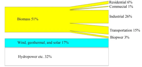
To understand the status quo of the U.S. renewable energy portfolio, we created a diagram using data from Table A17 of the EIA Annual Energy Outlook 2012 [AEO (2012)], as shown in Figure 2.1. Biomass was the resource for 51% of the total renewable energy consumed in 2012 (8.4 quadrillion Btu)1 in five sectors: residential 6%, commercial 1%, industrial 26% (collectively referred to as R.C.I.), transportation (biofuel) 15%, and biopower 3%. Wind 15%, geothermal 2%, and solar 0.4% (collectively referred to as W.G.S.) accounted for 17% and hydropower 32% of the total renewable energy portfolio.
Figure 2.1: The U.S. renewable energy portfolio in 2012. Data from AEO (2012)
The RPS and RFS2 policy drivers, along with others such as the production tax credits (PTC) or investment tax credits (ITC), will drive the U.S. renewable energy portfolio in 2035 very different than it was in 2012. RPS targets on increasing renewable electricity,
ing biopower, W.G.S. power, and hydropower [Wiser et al. (2007)]. As of April 2013, thirty states have established RPS mandates and eight have set similar but non-binding goals [DSIRE (2013d)]. So far, the RPS rules in different states are all unique. These rules differ by program structure, enforcement mechanism, classification of generating technologies in tiers, mandated percentages or MWh of renewable electricity generation, deadlines, and non-compliance penal-ties. There is a rich body of literature on the feasibility and potential impact of RPS.
Johnson and Moyer (2012) analyzed the Illinois RPS and suggested that full implemen-tation of the legislation in Illinois (and perhaps other states) is unlikely without “continued reductions in wind and solar costs and/or an unforeseen rise in wholesale electricity rates”. Cory and Swezey (2007) discussed the “hurdle of RPS rules that vary from state to state” that implementation of RPS must surmount to be successful. Carley (2009) found that “states with RPS policies do not have statistically higher rates of RE [renewable energy] share deployment than states without RPS policies.” On the contrary, Yin and Powers (2010) used a new mea-sure of policy stringency to argue that “RPS policies have had a significant and positive effect on in-state renewable energy development”. They also pointed out that allowing for free trade of renewable energy certificates “can significantly weaken the impact of an RPS”. Menza and Vachon (2006) also found RPS to be effective in “promoting the development of wind capacity.” Palmer and Burtraw (2005) compared the cost effectiveness of RPS, production tax credit, and cap-and-trade and concluded that cap-and-trade is more effective in achieving carbon emission reductions than the other two.
Renewable Fuel Standard (RFS) is a federal program designed to help protect public health and the environment and reduce the dependence on imported petroleum. Renewable fuels are defined as liquid or gaseous fuels derived from renewable biomass energy sources. A mandatory minimum volume of biofuel to be used in the national transportation fuel supply was estab-lished in 2005 with the Energy Policy Act. The initial standard mandated that the minimum usage volume of renewable fuel rise to 7.5 billion gallons2 by 2012. Two years later, the Energy Independence and Security Act of 2007 expanded the biofuel mandate to 36 billion gallons of (including 16 billion gallons for cellulosic and 20 billion gallons for non-cellulosic) biofuel to be
2
blended into transportation fuel by 2022 [Schnepf and Yacobucci (2010)]. This revised RFS is referred to as RFS2. A few recent studies have started to address the potential interactions of RFS2 with other policies. Jeffers et al. (2013) studied the bioenergy feedstock commodity mar-ket with three buyers: biopower, biofuel, and foreign exports. Their simulation model showed that either biofuel or overseas biomass demand could dominate the market under different policy settings. They also suggested that market competition can “effectively drive up prices for the biomass feedstocks and potentially exclude industries from the market”. Huang et al. (2013) studied the interactions of three policies: RFS2, low carbon fuel standard (LCFS), and a carbon price. They concluded that “the addition of a LCFS to the RFS increases the share of second generation biofuel; the addition of a carbon price to these policies encourages fuel conservation; these combined policies significantly increase the reduction in GHG emissions; [and] they also achieve greater energy security and economic benefits than the RFS alone”.
Our study makes a new contribution to the existing literature by pioneering the analysis on the interactions between RPS and RFS2. In particular, we are motivated to seek answers to the following questions that have not been elucidated by previous studies. These questions are difficult to address without looking at how the two policies (along with others) jointly affect the entire renewable energy market along all resource, geographical, and temporal dimensions.
Q1: What are the potential interactions between RPS and RFS2?
Q2: Under RPS and RFS2, how will the competition for biomass between biopower generation and biofuel production progress in the next two decades?
Q3: Under RPS and RFS2, what is the outlook of renewable energy portfolio in the U.S.?
Q4: How will different states’ unique renewable energy portfolios evolve in the next two decades?
2.2 Model
In order to address the five questions that motivated this study, we constructed an opti-mization model to describe the overarching interactions within the complex renewable energy portfolio from resource, geographical, and temporal dimensions. First, we include all major renewable energy resources (biomass, W.G.S., and hydro) and demand sectors (biopower, non-cellulosic and non-cellulosic biofuel, W.G.S. power, and hydropower) into the modeling framework. As such, the prediction of renewable energy portfolio from our model resulted from careful eval-uation of costs (capital investment cost, operating and maintenance costs, and non-compliance penalties) and benefits (sales revenue and tax credits) of each technology rather than over-simplifying presumptions. Second, our model treats all 50 states and Washington D.C. as 51 separate entities, each having their own reserves of renewable energy resources and unique RPS requirements (mandates, goals, or neither). Nevertheless, our model also captures the interac-tions among different states, including truck transportation of biomass and RFS2 compliances. Third, we use a 23-year modeling horizon, which allows us to accommodate practical consid-erations of market trends before and after RPS and RFS2 deadlines as well as time value of money.
We made several major simplifying assumptions, some of which are due to lack of good data and others are believed to be necessary to maintain tractability of the model without significantly compromising the credibility of the results. First, our optimization model adopts a centralized and coordinative planning perspective by maximizing the net present value of the total profit (benefits less costs) of the U.S. renewable energy industry, which is used to approximate the investment and operating decisions for all states across all renewable energy sectors throughout the modeling horizon. In reality, investment and operating decisions are made by multiple decision makers in electricity and transportation fuel markets to serve their own objectives, some competitively and others in coordination. Thus, game theoretic models would be able to better describe such market behavior. However, game theoretic models would not only require much higher modeling granularity and more sophisticated database but also encounter much more complicated computational challenges such as the tractability, existence,
and uniqueness of a market equilibrium. Our optimization model avoids such problems by assuming that the invisible hand of economy will direct the overall flow of capital and natural resources in the most efficient manner towards cost minimization and profit maximization for the entire industry. Second, our model is deterministic, not taking uncertainty into explicit consideration. To address the concerns raised in Q5 regarding uncertainty and its potential impact on the renewable energy output, we conduct a sensitivity analysis by examining the impact of dozens of parameters on the results. Third, our model treats several factors as known parameters rather than decision variables due to their lack of unforeseeable interactions with the rest of the model. For example, demands of biomass energy in the R.C.I. sectors are not directly affected by either RPS or RFS2, thus their projections in the next two decades are treated as known. Non-cellulosic biofuel (mostly corn ethanol and soybean diesel) production is also assumed to exactly meet the RFS2 requirement due to abundant existing capacity of these conventional biofuel production facilities. Fourth, we do not treat hydropower as RPS eligible for any state. Since the goal of the RPS is to encourage new investment in renewable energy, and most hydroelectric facilities were installed decades ago, most states place certain restrictions on hydropower by capacity, vintage, or technology, and some do not count hydropower at all. Some legislations regarding the RPS eligibility of hydropower are difficult to formulate in the model or require more detailed data than what is publicly available.
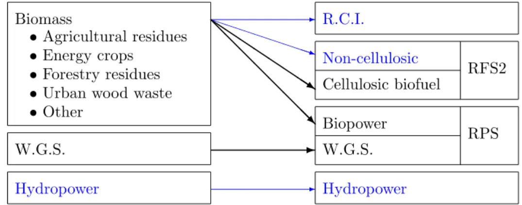
Along the resource dimension of our optimization model as described above, the structure of the model is depicted in Figure2.2, which exactly represents the major resources and demand sectors of the U.S. renewable energy portfolio as diagramed in Figure2.1. Following the cate-gorization in Haq and Easterly (2006), we consider four major types of biomass: agricultural residues, energy crops, forestry residues, and urban wood waste. The “other” category mostly accounts for conventional biomass resources such as corn or soybean. Due to the aforemen-tioned reasons, the R.C.I. sectors, non-cellulosic biofuel, and hydropower are treated as known parameters (all colored in blue) and are not formulated as decision variables in the model. To accurately incorporate RPS policy, our model sets a separate constraint for each RPS state and for each eligible renewable energy defined in the legislation. Non-compliance penalties for
different types of renewable energy in different states are also captured in the model. The RFS2 policy is similarly formulated as a soft constraint with a penalty for non-compliances.
Biomass
• Agricultural residues • Energy crops
• Forestry residues • Urban wood waste • Other W.G.S. Hydropower R.C.I. Non-cellulosic Cellulosic biofuel RFS2 Biopower W.G.S. RPS Hydropower -P P P P P P PPq -Q Q Q Q Q Q QQs @ @ @ @ @ @ @@R
-Figure 2.2: Modeling structure
Using the sets, parameters, and decision variables defined in Appendix A, the mathematical formulation of our optimization model is presented as follows.
max ζ =P
v,j,t(1 +r)(t0−t)(βj,t+ϕv,t)xv,j,t+Pj,t(1 +r)(t0−t)(βtF+ϕFt)xFj,t (2.1)
−P
u,j,t(1 +r)(t0−t)cu,j,txu,j,t−
P
u,i6=j,t(1 +r)(t0−t)πi,j,tyu,i,j,t (2.2)
−P v,j,t(1 +r)(t0−t)(cv,j,t+fv,j,t)xv,j,t− P j,t(1 +r)(t0−t)cFj,txFj,t (2.3) −P v,j,t(1 +r)(t0−t)lv,j,t(1−λv,t)zv,j,t− P j,t(1 +r)(t0−t)lFj,t(1−λFt)zFj,t (2.4) −P j,t,k(1 +r)(t0−t)µj,t,ksj,t,k−Pt(1 +r)(t0−t)µFtsFt (2.5) s.t. P uρu
xu,j,t+Pi6=jyu,i,j,t−Pi6=jyu,j,i,t
≥dj,t+ 1.45×10⁻²xbiomass,j,t+ 2.90×10⁻⁴xFj,t ∀j, t (2.6)
xu,j,t+Pi6=jyu,i,j,t≥Pi6=jyu,j,i,t ∀u, j, t (2.7)
pv,j,t =pv,j,(t−1)+zv,j,t ∀v, j, t (2.8)
pFj,t =pFj,(t−1)+zj,tF ∀j, t (2.9)
xu,j,t ≤pu,j,t ∀u, j, t (2.10)
xv,j,t ≤8760αvpv,j,t ∀v, j, t (2.11)
zv,j,t≤Mv,j,t ∀v, j, t (2.13) zj,tF ≤Mj,tF ∀j, t (2.14) P vqv,j,kxv,j,t+sj,t,k ≥ηj,t,kej,t ∀j, t, k (2.15) P jxFj,t+sFt ≥θt ∀t (2.16)
all decision variables≥0 (2.17)
The objective function (2.1)-(2.5) of the model is to maximize the net present value of the total profit (revenue less cost) of the renewable energy industry. In (2.1), the first term is the total revenues from sales (β) and production tax credits (ϕ) for W.G.S. power and biopower generation (x), and the second term is revenue for cellulosic biofuel production. The discount factorris used to calculate the present value of future cash flows. The eight cost terms in (2.2 )-(2.5) are for, respectively, biomass production, biomass transportation, renewable electricity generation (variable cost cplus fixed costf), biofuel production, capital investment (adjusted by investment tax credit) in new renewable power plants, capital investment (adjusted by investment tax credit) in biofuel production facilities, penalties for RPS non-compliances, and penalties for RFS2 shortfalls. Constraint (2.6) requires that the amount of biomass production and imports minus exports must exceed demand from R.C.I. sectors, biopower generation, and biofuel production (all converted to BBtu). Constraint (2.7) sets the combined amount of biomass production and imports as the upper limit for exports. Equations (2.8) and (2.9) update the yearly capacities of renewable electricity generation (in MW) and biofuel production (in gallon) to account for new additions. Constraints (2.10)-(2.12) define the available capacity for biomass production, renewable electricity generation, and biofuel production, respectively. Constraints (2.13) and (2.14) set the upper bounds of new capacities for investment in renewable power plants and biofuel production facilities that can be realistically put in due to limitations in manufacturing capability, resource (material, labor, funds, etc.) availability, and legislative requirements. Constraints (2.15) and (2.16) set RPS and RFS2 requirements. The RFS2 target is an aggregate for all states, whereas RPS mandates are specified for each state and each type of renewable energy. The binary parameterqv,j,k indicates whether or not renewable electricity
type v is included in tier k of state j’s RPS legislation. All decision variables are required to be non-negative in Constraint (2.17).
2.3 Results
The linear program model (2.1)-(2.17) contains 261,603 decision variables and 22,380 con-straints. The entire data set take more than 1 MB of hard drive space. It was programmed in GAMS and solved to optimality in a few seconds on a desktop computer with standard configurations. Data used for all sets and parameters in the model are explained in Appendix B. We present our modeling results by answering the five motivating questions.
Q1: What are the potential interactions between RPS and RFS2?
A1: We assess the potential interactions between RPS and RFS2 by comparing the modeling results with four cases of policy implementation: no policy (case 1), RPS only (case 2), RFS2 only (case 3), and both policies (case 4). Numerical results are summarized in Table
2.1. Without RFS2, RPS would increase 65.19 billion kWh/year of W.G.S. power and 25.85 billion kWh/year of biopower, averaged between 2013 and 2035. This effect repre-sents an increase of the nationwide renewable electricity portfolio (excluding hydropower) from 6.87% in 2013 to 11.47% in 2035. On the other hand, without RPS, RFS2 would in-crease nationwide cellulosic biofuel production by an average of 7.69 billion gallons/year. The interaction of the two policies reduces the contributions of both. Specifically, due to the competition for biomass from RFS2, a yearly average of 7.70 million tons of biomass that would have been used to generate biopower under RPS will be used to produce cel-lulosic biofuel instead. Reversely, due to the competition for biomass from RPS, a yearly average of 5.01 million tons of biomass that would have been used to produce cellulosic biofuel under RFS2 will be used to generate biopower instead. We also point out that the interactions between RPS and RFS2 have little impact on W.G.S.; they only affect the total amount of biomass production and the allocation of the biomass resource for biopower and cellulosic biofuel.
Table 2.1: Modeling results in four cases
Case 1 Case 2 Case 3 Case 4
RPS X X
RFS2 X X
Average W.G.S. power generation (billion kWh/year) from 2013 to 2035
320.68 385.87 320.68 386.01 Average biopower generation (billion
kWh/year) from 2013 to 2035
0.17 26.01 0.17 16.78
Average biomass used for biopower generation (million ton/year)
0.14 21.68 0.14 13.98
Average cellulosic biofuel production (billion gallon/year) from 2013 to 2035
0.02 0.02 7.71 7.41
Average biomass used for cellulosic biofuel production (million ton/year)
0.32 0.32 128.54 123.53
Q2: Under RPS and RFS2, how will the competition for biomass between biopower generation and biofuel production progress in the next two decades?
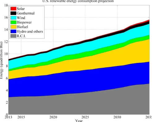
A2: To address this question, we plot in Figure 2.3 the projection of four sectors of renew-able energy consumption in the U.S. that are based on biomass resources. The R.C.I. projection is adopted from AEO (2012), the non-cellulosic biofuel production is assumed to exactly meet the RFS2 requirements, and the projections for biopower and cellulosic biofuel are from our modeling results. The figure shows that biomass based renewable energy will increase by 69% in the next two decades, with R.C.I. and non-cellulosic biofuel accounting for a combined 95% and 87% in 2013 and 2035, respectively. The competi-tion for biomass between biopower and biofuel is expected to turn sharply from biopower being the dominating pathway to the opposite. Biopower is expected to shrink by 67% over the next two decades due to lack of cost competitiveness compared to W.G.S. power generation technologies as well as the distraction from RFS2. This result is consistent with the findings from Dassanayake and Kumar (2012) in which triticale straw-based biopower generation is less economically competitive than coal-based electricity genera-tion. Driven by RFS2, annual production of cellulosic biofuel is expected to surge from 0.14 billion gallons in 2013 to 8.91 billion gallons in 2022 (7.09 billion gallons short of the
16 billion-gallon target) and then 8.81 billion gallons in 2035. The downturn of cellulosic biofuel production after 2023 is due to the assumed expiration of the cellulosic biofuel producer tax credit in 2022.
Figure 2.3: Projection of biomass based renewable energy consumption in the U.S. Results from our model are combined with data from AEO (2012).
Q3: Under RPS and RFS2, what is the outlook of renewable energy portfolio in the U.S.?
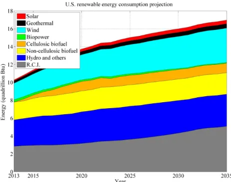
A3: Table A17 in the Annual Energy Outlook 2012 [AEO (2012)] as well as our modeling results can be used to address this question. In Figure 2.4, we plot the EIA projection of renewable energy consumption broken into seven categories. For the purpose of model validation, we also plot the same seven categories of projection with an additional dif-ferentiation of cellulosic and non-cellulosic biofuel from our modeling results in Figure
2.5. Since our model does not include projections for non-cellulosic biofuel, hydropower, and R.C.I., we use the same data for those sectors from AEO (2012) in Figure2.5. The overall trend of our projections is consistent with the EIA results. However, we are more
optimistic than EIA on the growth of W.G.S. power but less so on biopower. In fact, EIA expects biopower to grow 2.4-fold between 2013 and 2035, whereas we predict a 67% shrink. Moreover, we are more optimistic than EIA about the growth of cellulosic biofuel production before the 2022 deadline, but we expect the production to stay at the same level with a slight fallback afterwards rather than continuing to grow throughout 2035 as EIA projected. According to Annual Energy Outlook 2012, 22.1 billion gallons of biofuel (including cellulosic and non-cellulosic) will be produced in 2022, which is 13.9 billion gallons short of the RFS2 target. We predicted 28.91 billion gallons biofuel production in 2022, including 8.91 billion gallons cellulosic (by modeling results) and 20 billion gallons non-cellulosic (by assumption) biofuels, which is 7.09 billion gallons short of the target.
Figure 2.4: Projection of renewable energy consumption in the U.S. from Table A17 in AEO (2012) for the reference case
Q4: How will different states’ unique renewable energy portfolios evolve in the next two decades?
A4: Figures 2.6-2.10 show the trends of top states in wind, geothermal, solar, biopower, and cellulosic biofuel, respectively. Each curve represents the trajectory of a certain type of
Figure 2.5: Projection of renewable energy consumption in the U.S. from our model under the base case scenario combined with partial data from AEO (2012).
renewable energy generation between 2013 and 2035 in a specified state. Whereas most states show an increasing trend of renewable energy generation, biopower is shrinking and losing the competition to cellulosic biofuel. Figure 2.11 plots the renewable energy portfolios of top 30 renewable energy generating states, which is broken into four types of resources: wind, geothermal, solar, and biomass (for biopower and cellulosic biofuel). Non-cellulosic biofuel or hydropower is not included in Figure 2.11.
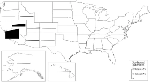
Figure 2.7: Geothermal power generation in top 10 states between 2013 and 2035.
Figure 2.8: Solar power generation in top 20 states between 2013 and 2035.
Figure 2.10: Cellulosic biofuel production in top 20 states between 2013 and 2035.
Figure 2.11: Renewable energy portfolios in top 30 states broken into four types of resources averaged between 2013 and 2035, excluding biomass for non-cellulosic biofuel production.
Q5: What factors is the U.S. renewable energy portfolio most sensitive to?
A5: To quantify the sensitivity of renewable energy production with respect to multiple pa-rameters, we define three scenarios each comprising of a set of values for these parameters: base case, optimistic, and pessimistic scenarios. The optimistic and pessimistic scenarios are defined in such a way that the nationwide total renewable energy generation would be increased and decreased with respect to the base case, respectively. The objective of
this analysis is to identify parameters that would have the most significant impact on the modeling results. Answers A1-A4 were all based on the base case scenario, which we believe represents the most likely realization of the uncertain parameters. Parameter values for the base case scenario are described in Appendix B. The changes of parameter values for these two scenarios are described as follows.
Optimistic scenario: Seven cost parameters (cu,j,t, cv,j,t, cFj,t, πi,j,t, fv,j,t, lv,j,t, lj,tF) are
re-duced by 20% with respect to the base case. Two revenue parameters (βj,t, βtF) are
increased by 20%. The investment limits Mv,j,t and Mj,tF are increased by 20%.
Two penalty parameters for RPS and RFS2 non-compliances (µj,t,k, µFt) are
in-creased by 50%. Four expiration dates of investment and production tax credits (ϕv,t, ϕFt, λv,t, λFt) are all extended to 2035.
Pessimistic scenario: The seven cost parameters are increased by 20% and the two revenue parameters are reduced by 20%. The investment limits Mv,j,t andMj,tF are
decreased by 20%. The two penalty parameters are reduced by 50%. The four expiration dates of tax credits (ϕv,t, ϕFt, λv,t, λFt) are expedited to 2023, 2013, 2016,
and 2013, respectively. These are the expiration dates set by the current regulations, assuming no further extensions.
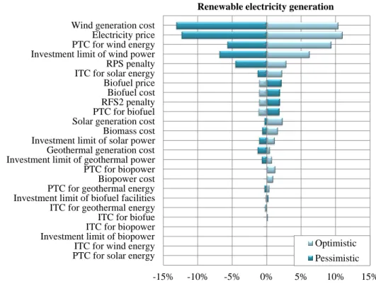
Our sensitivity analysis results are plotted in Figures2.12-2.17. In each figure, the effects of all uncertain parameters on one output in the optimistic and pessimistic scenarios are shown against the base case, and the effects are ranked from the largest on top to the smallest at the bottom. Each bar in Figures2.12-2.17is obtained by running the model (2.1)-(2.17) with only one change in the parameter (or set of parameters) specified on the left-hand-side of the figures.
Figure2.12shows the sensitivity of the total renewable electricity generation with respect to the uncertain parameters we identified. Four factors could affect the total generation by more than 5%: electricity price, wind generation cost (including investment cost and variable cost), PTC for wind, and investment limit on wind. These results suggest that wind energy will play an important role in shaping the renewable electricity development.
Its economic or technological improvement and policy changes will have more impact than any other type of renewable energy on total renewable electricity generation.
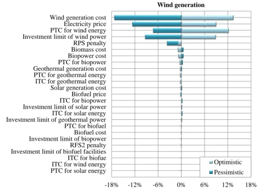
Figure 2.13 suggests that wind power generation is most sensitive to five factors: wind generation cost, electricity price, renewal/expiration of PTC for wind, investment limit of wind power, and RPS penalty. Interestingly, either increasing or decreasing RPS penalty will reduce wind power generation. If RPS penalty is decreased, then all renewable electricity generation will fall. On the other hand, if RPS penalty is increased, then solar power and biopower will increase, as can be seen in Figures2.15and2.16, but wind power will fall. These results demonstrate the interactions between multiple renewable energy resources and technologies in response to policy changes.
Figure 2.14 suggests that geothermal power generation is most sensitive to five factors: geothermal generation cost, investment limit of geothermal power, electricity price, and renewal/expiration of PTC and ITC for geothermal. RPS penalties play a similar role as in wind generation. Favorable changes in wind generation cost and investment limit of wind power also affect geothermal generation, but in the opposite direction as they have on wind generation. This is due to the substitutability of W.G.S. resources in fulfilling RPS requirements.
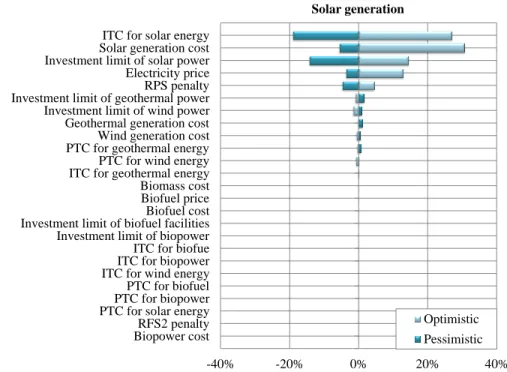
Figure 2.15 suggests that solar power generation is most sensitive to five factors: re-newal/expiration of ITC for solar, solar generation cost, investment limit of solar power, electricity price, and RPS penalty. For solar, the increase (or decrease) of RPS penalty does intuitively increase (or decrease) solar power generation. Favorable changes for competing technologies also have negative effects on solar power.
Figure2.16suggests that many factors could significantly affect biopower generation. We make two interesting observations. First, nine factors could increase biopower generation by 80% or more, and seven of them could also decrease the generation by 50% or more. Second, biopower generation is very susceptive to the competition from cellulosic biofuel. All favorable (or non-favorable) changes for cellulosic biofuel will negatively (or positively) affect biopower generation, and four of these factors could decrease (or increase) biopower
generation by above 50% (or 100%). In contrast, the same set of factors have much less effect (below 20%) in the more mature W.G.S. technologies.
Figure2.17suggests that biofuel production is most sensitive to five factors: renewal/expiration of PTC for biofuel, biofuel price, biofuel cost, RFS2 penalty, and biomass cost, all of which could increase or decrease cellulosic biofuel production by at least 32% and up to 89%. In contrast to biopower, cellulosic biofuel production is much less sensitive to competition from biopower and other types of renewable energy policies.
-15% -10% -5% 0% 5% 10% 15%
PTC for solar energy ITC for wind energy Investment limit of biopower ITC for biopower ITC for biofue ITC for geothermal energy Investment limit of biofuel facilities PTC for geothermal energy Biopower cost PTC for biopower Investment limit of geothermal power Geothermal generation cost Investment limit of solar power Biomass cost Solar generation cost PTC for biofuel RFS2 penalty Biofuel cost Biofuel price ITC for solar energy RPS penalty Investment limit of wind power PTC for wind energy Electricity price Wind generation cost
Optimistic Pessimistic
Renewable electricity generation
-18% -12% -6% 0% 6% 12% 18% PTC for solar energy
ITC for wind energy ITC for biofue Investment limit of biofuel facilities RFS2 penalty Investment limit of biopower Biofuel cost PTC for biofuel Investment limit of geothermal power ITC for solar energy Investment limit of solar power ITC for biopower Biofuel price Solar generation cost ITC for geothermal energy PTC for geothermal energy Geothermal generation cost PTC for biopower Biopower cost Biomass cost RPS penalty Investment limit of wind power PTC for wind energy Electricity price Wind generation cost
Optimistic Pessimistic
Wind generation
Figure 2.13: Sensitivity of wind power generation.
-18% -12% -6% 0% 6% 12% 18%
Biomass cost Biopower cost PTC for solar energy PTC for biopower PTC for biofuel ITC for wind energy ITC for biopower ITC for biofue Investment limit of biopower Investment limit of biofuel facilities RFS2 penalty Investment limit of solar power Biofuel cost Biofuel price PTC for wind energy Solar generation cost ITC for solar energy RPS penalty Investment limit of wind power Wind generation cost ITC for geothermal energy PTC for geothermal energy Electricity price Investment limit of geothermal power Geothermal generation cost
Optimistic Pessimistic
Geothermal generation
-40% -20% 0% 20% 40% Biopower cost
RFS2 penalty PTC for solar energy PTC for biopowerPTC for biofuel ITC for wind energyITC for biopower ITC for biofue Investment limit of biopower Investment limit of biofuel facilities Biofuel cost Biofuel price Biomass cost ITC for geothermal energy PTC for wind energy PTC for geothermal energy Wind generation cost Geothermal generation cost Investment limit of wind power Investment limit of geothermal power RPS penalty Electricity price Investment limit of solar powerSolar generation cost ITC for solar energy
Optimistic Pessimistic
Solar generation
Figure 2.15: Sensitivity of solar power generation.
-200% -100% 0% 100% 200%
Geothermal generation costSolar generation cost PTC for geothermal energy PTC for solar energy ITC for wind energy ITC for geothermal energyITC for solar energy Investment limit of geothermal power Investment limit of solar power Investment limit of biopowerITC for biofue ITC for biopower PTC for wind energy Investment limit of biofuel facilities Wind generation cost Investment limit of wind power PTC for biopower Biopower cost RFS2 penalty PTC for biofuel Biofuel cost Electricity price Biomass costBiofuel price RPS penalty
Optimistic Pessimistic
Biopower generation
-100% -50% 0% 50% 100% PTC for solar energy
ITC for wind energy ITC for geothermal energy ITC for biopower Investment limit of biopower PTC for geothermal energy Wind generation cost Geothermal generation cost Solar generation cost PTC for wind energy Investment limit of geothermal power Investment limit of solar power ITC for solar energy Investment limit of wind power PTC for biopower Biopower cost Electricity price RPS penalty ITC for biofue Investment limit of biofuel facilities Biomass cost RFS2 penalty Biofuel cost Biofuel price PTC for biofuel Optimistic Pessimistic
Cellulosic biofuel production
Figure 2.17: Sensitivity of cellulosic biofuel production.
2.4 Conclusions
Our study focused on the potential competition for biomass from RPS driven biopower generation and RFS2 driven biofuel production as well as other interactions between these two policies. As perhaps the first study on this topic, our model has several unique strengths that make it particularly appropriate to address the five important questions Q1-Q5. First, our model takes a systems perspective of the entire renewable energy portfolio. On the resource dimension, availability of multiple renewable energy resources, projection of all major demand sectors in the industry, and investment and operating costs of different generation/production technologies are incorporated. On the geographical dimension, the differences of 50 states and Washington D.C. in renewable energy resource abundance, demand, RPS policies (including different definitions of tiers, deadlines, and penalties), and investment constraints were all explicitly taken into account. On the temporal dimension, a 23-year modeling horizon was used to observe how the U.S. renewable energy industry evolves to pass one deadline after another
set by various RPS and RFS2 legislations. Second, our model is computationally tractable. Efficient linear programming algorithms and software can solve the model to optimality within a few seconds, which allows the model to be solved multiple times to answer what-if questions and for sensitivity analysis. Third, most of the parameters used in our computational study are from publicly available database; when certain data are unavailable, assumptions were carefully made and validated through multiple channels to fill in the gap. Fourth, our computational experiment is conveniently repeatable and extensible for further analysis. All parameters, variables, objective, and constraints of the model are explained; all of the data used as well as their sources are described in Appendices A and B. As a result, improvement can be easily made if additional features of the policy become the focal point of a new research question or more detailed data become available.
Results from our model suggest that cellulosic biofuel production will quickly dominate the competition for biomass against biopower generation. This is because the biomass production and biopower generation costs are higher than those for W.G.S. power, whereas cellulosic biofuel production faces a stringent RFS2 mandate with no cheaper substitution. The renewable energy portfolios in 50 states and Washington D.C. could vary significantly, and they all have their unique trajectories throughout 2035. Our sensitivity analysis reveals that W.G.S. power generation is relatively robust with respect to various uncertain factors, whereas biopower and biofuel are much more susceptible to uncertainty associated with (investment, generation, production) costs, (electricity and transportation fuel) prices, and policies. These analysis results also suggest that the interactions between RPS and RFS2 will have more impact on biopower than on biofuel.
As pointed out in the Introduction section, we made several simplifying assumptions in the model, which may affect the accuracy of our results to some extent. It would be difficult to integrate the strategic behavior of investors in the renewable energy markets without switching to a completely different modeling approach, which may have limitations of its own. However, we expect that more credible results could be obtained by feeding the model with more accurate data, such as investment and operating costs in different states. Moreover, the model can
be extended to incorporate additional features, such as explicit modeling of the eligibility of hydropower in different RPS legislations, given clarification of policy and availability of data.
2.5 Appendix A
Sets
Notation Definition
J Set of 50 states in the U.S. and Washington D.C. JRPS Set of 38 U.S. states with RPS (30) or RPG3(8)
Kj Set of tiers of RPS policy for statej∈ JRPS
T Set of years within modeling horizon,T ={t1, t2, ..., tT}, whereT is
the number of years in the modeling horizon.
U Set of four major types of biomass
V Set of four major types of renewable electricity resources
Parameters
Notation Definition Unit
cu,j,t Biomass production cost of typeu∈ U in statej∈ J in year
t∈ T
$/ton
πi,j,t Biomass transportation cost from state i ∈ J to j ∈ J in
yeart∈ T
$/(ton mile)4
cv,j,t/fv,j,t Renewable energy generation variable/fix cost of typev ∈ V
in statej∈ J in year t∈ T
$/MWh
cFj,t Cellulosic biofuel production cost in statej∈ J in yeart∈ T $/gallon
lv,j,t Capital investment cost of renewable electricity generation of
typev ∈ V in statej∈ J in year t∈ T
$/MW
lFj,t Capital investment cost of cellulosic biofuel facilities in state
j∈ J in yeart∈ T
$/gallon
βj,t Average wholesale electricity price in state j ∈ J in year
t∈ T
$/MWh
βFt Average biofuel price in yeart∈ T $/gallon
ϕv,t Production tax credit for renewable electricity generation of
typev ∈ V in yeart∈ T
$/MWh
ϕFt Cellulosic biofuel producer tax credit in yeart∈ T $/gallon
3Renewable Portfolio Goal 4
λv,t Investment tax credit as a percentage discount of capital
in-vestment of renewable electricity generation of typev∈ V in yeart∈ T
unitless
λFt Investment tax credit as a percentage discount of capital investment of cellulosic biofuel production facilities in year
t∈ T
unitless
µj,t,k Penalty for non-compliance with RPS tier k ∈ Kj in state
j∈ J in yeart∈ T
$/MWh
µFt Penalty for non-compliance with RFS2 in yeart∈ T $/gallon
r Discount rate unitless
ρu Conversion factor of 1 ton biomass of type u∈ U to 1 BBtu BBtu/ton
dj,t Demand of biomass from the R.C.I. sectors in statej∈ J in
yeart∈ T
BBtu
pu,j,t Availability of biomass type u ∈ U in state j ∈ J in year
t∈ T
ton
pv,j,t0 Capacity of renewable electricity generation of typev∈ V in
statej ∈ J in year t0, which is one year before the first year in the modeling horizon
MW
pFj,t0 Capacity of cellulosic biofuel production in state j ∈ J in yeart0
gallon
αv Capacity factor of renewable energy unitless
Mv,j,t Maximum level of new investment in renewable energy
facil-ities in statej ∈ J in yeart∈ T
MW
Mj,tF Maximum level of new investment in cellulosic biofuel facili-ties in statej∈ J in year t∈ T
gallon
qv,j,k Indicator of whether (qv,j,k = 1) or not (qv,j,k = 0) renewable
energy type v ∈ V is included in the definition of RPS tier
k∈ Kj by state j∈ JRPS
unitless
ej,t Annual electricity consumption projection in state j ∈ J in
yeart∈ T
MWh
ηj,t,k RPS requirements or goals of tierk∈ Kj in state j ∈ JRPS
in yeart∈ T
unitless
θt RFS2 requirements in yeart∈ T gallon
Decision variables
Notation Definition Unit
ζ Net present value of total profit throughout the modeling horizon
xu,j,t Biomass production of type u ∈ U in state j ∈ J in year
t∈ T
ton
xv,j,t Renewable electricity generation of typev∈ V in statej∈ J
in yeart∈ T
MWh
xFj,t Cellulosic biofuel production in statej∈ J in year t∈ T gallon
yu,i,j,t Amount of biomass transportation of typeu∈ U from state
i∈ J toj∈ J in year t∈ T
ton
zv,j,t New capacity of renewable electricity generation of typev ∈
V in state j∈ J in yeart∈ T
MW
zj,tF New capacity of cellulosic biofuel production in statej ∈ J
in yeart∈ T
gallon/year
pv,j,t Renewable electricity generation capacity of type v ∈ V in
statej∈ J in year t∈ T
MW
pFj,t Cellulosic biofuel production capacity in statej ∈ J in year
t∈ T
gallon/year
sj,t,k Renewable electricity generation shortfall of RPS
require-ments for tier k∈ Kj in statej∈ JRPS in year t∈ T
MWh
sFt Cellulosic biofuel production shortfall of RFS2 requirements in yeart∈ T
gallon
2.6 Appendix B
Sets
Notation Data or data source
J Data from USA.gov (2013) were used.
JRPS Data from DSIRE (2013b) were used.
Kj Data from DSIRE (2013b) were used.
T T ={2013, ...,2035}.
U U = {agricultural residues, energy crops, forestry residues, urban wood waste/mill residues}, as defined in Haq and Easterly (2006). V V ={wind,geothermal,solar,biomass}.
Parameters
Notation Data or data source
cu,j,t We assume $96/ton for all types of biomass for all states and a 3.5%
annual increase (based on information obtained from personal con-tact with biofuel companies and research experience).