Variable Selection in Multivariate Multiple
Regression
by
c
⃝Anita Brobbey
A thesis submitted to the School of Graduate Studies in partial fulfillment of the requirement for the Degree of
Master of Science
Department of Mathematics and Statistics Memorial University
Abstract
Multivariate analysis is a common statistical tool for assessing covariate effects when only one response or multiple response variables of the same type are collected in experimental studies. However with mixed continuous and discrete outcomes, traditional modeling approaches are no longer appropriate. The common approach used to make inference is to model each outcome separately ignoring the potential correlation among the responses. However a statistical analysis that incorporates as-sociation may result in improved precision. Coffey and Gennings (2007a) proposed an extension of the generalized estimating equations (GEE) methodology to simul-taneously analyze binary, count and continuous outcomes with nonlinear functions. Variable selection plays a pivotal role in modeling correlated responses due to large number of covariate variables involved. Thus a parsimonious model is always de-sirable to enhance model predictability and interpretation. To perform parameter estimation and variable selection simultaneously in the presence of mixed discrete
iii
and continuous outcomes, we propose a penalized based approach of the extended generalized estimating equations. This approach only require to specify the first two marginal moments and a working correlation structure. An advantageous feature of the penalized GEE is that the consistency of the model holds even if the working correlation is misspecified. However it is important to use appropriate working cor-relation structure in small samples since it improves the statistical efficiency of the regression parameters. We develop a computational algorithm for estimating the pa-rameters using local quadratic approximation (LQA) algorithm proposed by Fan and Li (2001). For tuning parameter selection, we explore the performance of unweighted Bayesian information criterion(BIC) and generalized cross validation (GCV) for least absolute shrinkage and selection operator(LASSO) and smoothly clipped absolute deviation (SCAD). We discuss the asymptotic properties for the penalized GEE esti-mator when the number of subjects n goes to infinity. Our simulation studies reveal that when correlated mixed outcomes are available, estimates of regression parame-ters are unbiased regardless of the choice of correlation structure. However, estimates obtained from the unstructured working correlation (UWC) have reduced standard errors. SCAD with BIC tuning criteria works well in selecting important variables. Our approach is applied to concrete slump test data set.
Contents
Abstract ii
List of Tables vii
List of Figures ix
Acknowledgements x
1 Introduction 1
1.1 Modelling Multiple Outcomes . . . 2
1.1.1 Literature Review . . . 2
1.2 Generalized Estimating Equation (GEE) . . . 5
1.2.1 Generalized Linear Models (GLM) . . . 5
1.2.2 Quasi-Likelihood (QL) Functions . . . 7
1.3 Variable Selection . . . 11
1.3.1 Sequential Approaches . . . 12
1.3.2 Information Criteria . . . 13
1.3.3 Penalized Likelihood Methods . . . 14
1.4 Motivation and Proposed Approach . . . 15
2 Penalized Generalized Estimating Equations(GEE) 18 2.1 Penalty Functions and Optimization . . . 19
2.1.1 LASSO . . . 19
2.1.2 SCAD . . . 21
2.1.3 Local Quadratic Approximation (LQA) Algorithm . . . 24
2.1.4 Standard Error . . . 26
2.2 GEE for Mixed Outcomes . . . 26
2.3 Variable Selection via Penalized GEE . . . 28
2.3.1 Correlation Structure . . . 30
2.3.2 Computational Algorithm . . . 31
2.3.3 Tuning Parameter Selection . . . 32
3 Simulation Studies 38
3.1 Simulation for Normal and Binary responses . . . 40 3.1.1 Case 1: Correlated Three Normal Responses . . . 40 3.1.2 Case 2: Correlated Two Normal and One Independent Binary
Responses . . . 41 3.1.3 Case 3 : Correlated Two Normal and One Binary Responses . 43 3.1.4 Case 4 : Correlated Two Normal and One Independent Count
Responses . . . 45
4 Case Studies 49
4.1 Concrete Slump Test Data . . . 49 4.1.1 Concrete Slump Test Data With Artificial Binary Response . 54
5 Conclusion 58
List of Tables
3.1 Simulations results for correlated normal responses (Case 1) with IWC. 41 3.2 Simulations results for correlated normal responses (Case 1) with UWC. 42 3.3 Simulations results for correlated normal and independent binary
re-sponses (Case 2) with IWC. . . 43 3.4 Simulations results for correlated normal and independent binary
re-sponses (Case 2) with UWC. . . 44 3.5 Simulations results for correlated normal and binary responses (Case
3) with IWC. . . 45 3.6 Simulations results for correlated normal and binary responses (Case
3) with UWC. . . 46 3.7 Simulations results for correlated normal and independent count
3.8 Simulations results for correlated normal and independent count re-sponses (Case 4) with UWC. . . 48
4.1 Correlation matrix for the responses . . . 51 4.2 Estimates of regression coefficients for slump (Y1), with standard error
in parentheses . . . 52 4.3 Estimates of regression coefficients for flow (Y2), with standard error
in parentheses . . . 53 4.4 Estimates of regression coefficients for compressive strength (Y3), with
standard error in parentheses . . . 54 4.5 Estimates of regression coefficients for slump (Y1), with standard error
in parentheses . . . 55 4.6 Estimates of regression coefficients for flow (Y2), with standard error
in parentheses . . . 56 4.7 Estimates of regression coefficients for binary compressive strength
List of Figures
2.1 Geometry of LASSO vs Ridge . . . 20 2.2 LASSO (top) and SCAD (down) penalty functions . . . 23
4.1 Scatter plot demonstrating visually the relationship between slump (Y1), flow (Y2) and compressive strength (CS) (Y3) . . . 51
Acknowledgements
I thank the Almighty God for his blessings throughout my education. I would like to express my deepest gratitude to my supervisor, Dr. Asokan Mulayath Variyath, for his patience, invaluable assistance, constructive criticisms and commitment which brought my thesis to a successful completion.
I gratefully acknowledge the funding received towards my MSc. from School of Graduate Studies, the Department of Mathematics & Statistics, and my supervisor in the form of graduate fellowships and teaching assistantships.
I also appreciate the assistance I received from the faculty members and staff of our department over the last two years, I am very grateful.
My warmest gratitude goes to my dear parents and guardians for their love, en-couragement and constant support.
Finally, I extend my sincere thanks to graduate students in the department, friends and loved ones who contributed in various ways to make this work a success.
Dedication
This thesis is dedicated to my father, Kofi Brobbey and to the memory of my mother, Agartha Opoku in appreciation for their unrelenting love and immense support.
Chapter 1
Introduction
In many applied science or public health studies, researchers are interested in modeling the relationship between response variable(s) and explanatory variables (independent variables). For example, in the well known Framingham Heart Study (Kannel et al., 1961), many covariates including age, sex, smoking status, cholesterol level, blood pressure were recorded on the participants over the years to identify risk factors for coronary heart disease. Despite the large number of covariates, some of them have no influence on the response variable. In some studies, the number of explanatory variables can be considerably large due to addition of interaction effects of covariates. If there are more than one response of interest, then the number of model parameters to be estimated will be much higher. Moreover, a model with all covariates may lead
1.1 Modelling Multiple Outcomes 2
to an over-fitting problem. Thus, parameter estimation and variable selection are two important problems in multivariate regression analysis. Selecting a smaller number of important variables results in a simpler and interpretable model. In this thesis, we address the variable selection problem in multivariate multiple regression models.
1.1
Modelling Multiple Outcomes
Multivariate multiple regression analysis is a common statistical tool for assessing covariate effects when only one response or multiple response variables are collected in observational or experimental studies. Many multivariate regression techniques are designed for univariate response cases. A common approach to dealing with multiple response variables is to apply the univariate response regression technique separately on each response variable ignoring the joint information among the responses. To solve this multi-response regression problem, several methodologies in generalized linear model (GLM) framework have been proposed in literature.
1.1.1
Literature Review
Breiman and Friedman (1997) proposed the curd and whey method that uses the cor-relation among response variables to improve predictive accuracy. They showed that
1.1 Modelling Multiple Outcomes 3
their method can outperform separate univariate regression approaches but did not address variable selection. In general, using multivariate multiple linear regression is more appropriate in investigating relations between multiple response (Goldwasser & Fitzmaurice 2006). The analysis of multivariate outcomes is especially challeng-ing when multiple types of outcomes are observed, the methodology is comparatively scarce when each response is to be modeled with a nonlinear function. However, multivariate outcomes of mixed types occur frequently in many research areas includ-ing dose-response experiment in toxicology (Moser et al 2005; Coffey & Genninclud-ings, 2007a, 2007b), birth defects in teratology (Sammel, Ryan & Legler, 1997) and pain in public health research (Von Korff et al 1992; Sammel & Landis, 1998). In the last three decades, methodologies for mixed-type outcomes includes using factorization ap-proaches based on extensions of the general location model proposed by Fitzmaurice and Laird (1997) and Liu and Rubin (1998). These likelihood based methodologies factor the joint distribution of the random variables as the product of marginal and conditional distributions, but can be unattractive because of their dependence on parametric distributional assumptions. Sammel et al. (1997) proposed a latent vari-able model for cross-sectional mixed outcomes using generalized linear mixed model with continuous latent variables, allowing covariate effects on both the outcomes and the latent variables. Muthen and Shedden (1999) proposed a general latent variable
1.1 Modelling Multiple Outcomes 4
modeling framework that incorporates both continuous and categorical outcomes and associates separate latent variables for outcomes of each type. Miglioretti (2003) also developed a methodology based on latent transition regression model for mixed outcomes. Other authors (Prentice and Zhao 1991; Rochon 1996; Bull 1998; Gray and Brookmeyer 2000; Rochon and Gillespie 2001) handled mixed outcomes through modification of generalized estimating equation (GEE) of Liang and Zeger (1986). Although some of these approaches (Lefkopoulou, Moore, and Ryan 1989; Contreras and Ryan 2000) may incorporate the use of GEEs for nonlinear models, none of the methodologies have formally extended the modeling of mixed discrete and contin-uous outcomes to nonlinear functions. Coffey and Gennings (2007a) proposed an extension of the generalized estimating equation (GEE) methodology to simultane-ously analyze binary, count, and continuous outcomes with nonlinear models that incorporates the intra-subject correlation. The methodology uses a quasi-likelihood framework and a working correlation matrix. The incorporation of the intra-subject correlation resulted in decreased standard errors for the parameters. In addition, Cof-fey and Gennings (2007b) developed a new application to the traditional D-optimality criterion to create an optimal design for experiments measuring mixed discrete and continuous outcomes that are analyzed with nonlinear models. These designs are to choose the location of the dose groups and proportion of total sample size that result
1.2 Generalized Estimating Equation (GEE) 5
in a minimized generalized variance. The designs were generally robust to different correlation structures. Coffey and Gennings (2007b) observed a substantial gain in efficiency compared to optimal designs created for each outcome separately when the expected correlation was moderate or large. In this thesis, we use the GEE approach (Coffey and Gennings, 2007a) and also conduct a series of simulations to investigate the performance of their method. Since we use GEE approach, we briefly review it in the next section.
1.2
Generalized Estimating Equation (GEE)
1.2.1
Generalized Linear Models (GLM)
Nelder and Wedderburn (1972) introduced the class of generalized linear models (GLMs) which extends ordinary model to encompass non-normal response distribu-tions and modeling of the mean. The distribution ofyis a member of an exponential family such as the Gaussian, binomial, Poisson or inverse-Gaussian. For a GLM, let E(y|X) denote the conditional expectation of the response variable, y given the covariates, X and g(·) denote a known link function then
1.2 Generalized Estimating Equation (GEE) 6
where β is the vector of unknown regression coefficients to be estimated. Gener-alized linear models consists of three components, the random, systematic and link component.
• A random component specifying the conditional distribution of the response variable Y given the explanatory variables X. The densities of the random component can be written in the form,
f(y|θ, ϕ) =exp(yθ−b(θ)
a(ϕ) +c(y, ϕ)
)
where a(·), b(·) and c(·) are arbitrary known functions, ϕ is the dispersion pa-rameter andθ is the canonical parameter of the distribution.
• Asystematic component specifying a linear predictor function. For each subject
i,
ηi(β) =xTi β.
• Alink function,g(·) defines the relationship between the linear predictorηi and
the mean µi of Yi.
1.2 Generalized Estimating Equation (GEE) 7
For GLMs, estimation starts by defining a measure of the goodness of fit between the observed data and the fitted values generated by the model. The parameter estimates are values that minimize the goodness-of-fit criterion, we obtain the parameter esti-mates by maximizing the likelihood of the observed data. The log-likelihood based on a set of independent observations y1, y2, y3, ..., yn with density f(yi;β) is
ℓ(µ;y) =
n
∑
i=1
logf(yi;β).
The goodness-of-fit criterion is
D(y;µ) = 2ℓ(y;y)−2ℓ(µ;y).
This is called the scaled deviance. Deviance is one of the methods used for model checking and inferential comparisons. The greater the scaled deviance, the poorer the fit.
1.2.2
Quasi-Likelihood (QL) Functions
Wedderburn (1974) proposed to use the quasi-score function, which assumes only a mean-variance relationship to estimate regression coefficients, β without fully speci-fying the distribution of the observed data, yi. The score equation is of the form,
S(β) = n ∑ j=1 Si(β) = n ∑ j=1 ( ∂µi ∂β )T V ar−1(yi;β, ϕ)(yi−µi(β)) = 0. (1.2)
1.2 Generalized Estimating Equation (GEE) 8
To obtain the score function, the random component in the generalized estimating equations was replaced by the following assumptions:
E[Yi] =µi(β),
Var[Yi] =Vi =a(ϕ)V(µi).
Consider independent vector of responses Y1, Y2, ..., Yn with common meanµ and
co-variance matrix a(ϕ)V(µ).
The quasi-likelihood function is
Q(µ;y) = n ∑ j=1 ∫ µ y y−t a(ϕ)V(t)dt. (1.3)
The quasi-score function is
S(β;y) = ∂Q ∂β = n ∑ j=1 y−µ a(ϕ)V(µ),
whereS(β;y) possess the following properties: replaced by the following assumptions:
E[S] = 0 Var[S] =−E ( ∂S ∂µ )
1.2 Generalized Estimating Equation (GEE) 9
These properties form the basis of most asymptotic theory for likelihood-based in-ference. Thus in general, S behaves like a score function and Q like a log-likelihood function. The quasi-score function, S(β;y) would be the true score function of β if
Yi’s have a distribution in the exponential family. We find the value βQL that
max-imizes Q by setting S(βQL;y) = 0,this is called QL estimating equations. In matrix
form, we can express the score equation as;
S(β;y) = D
TV−1(y−µ)
ϕ ,
where D is the n ×p matrix with (i, j)th entry ∂µi/∂βj,V is the n ×n diagonal
matrix with ith diagonal entry V(µi), y = (y1, y2, ..., yn), and µ = (µ1, µ2, ..., µn).
The covariance matrix of S(β) plays the same role as Fisher information matrix in the asymptotic variance of β;
In=DTV−1D,
V ar( ˆβ) =In−1.
These properties are based only on the correct specification of the mean and variance of Yi.
Method of moments is used for the estimation of a(ϕ).
a( ˆϕ) = 1 n−p n ∑ i=1 (yi−µˆi)2 V( ˆµi) = χ 2 n−p,
1.2 Generalized Estimating Equation (GEE) 10
where χ2 is the generalized Pearson statistics. As in the case of GLM, the quasi-deviance function corresponding to a single observation is
D(y;u) =−2σ2Q(µ;y) = 2
∫ y
µ
y−t
V(t)dt. (1.4)
The deviance function for the complete observation y when the observations are independent is defined as D(y:µ) =
n
∑
i=1
D(yi :µi)
1.2.3
Generalized Estimating Equation (GEE)
The GEE approach was first developed by Liang and Zeger (1986) for longitudinal data. Suppose we have a random sample of observations fromnindividuals. For each individuali we have a vector of responses Yi = (Yi1, Yi2, . . . , Yini)
′ and corresponding covariates Xi = (Xi′1, X ′ i2, . . . , X ′ ini) ′, where eachY
ij is a scalar andXij′ ap-vector. In
general, the components ofYi are correlated butYiandYkare independent for anyi̸=
kgiven the covariates. To model the relationship between the response and covariates one can use a regression model similar to the generalized linear model(GLM): (see equation (1.1)). The GEE approach suggests estimating β by solving the following estimating equation.(Liang and Zeger,1986)
S(β) =
n
∑
i=1
1.3 Variable Selection 11
whereDi =∂µiβ/∂β′andViis a working covariance matrix ofYiandVi =A1i/2R(α)A
1/2
i
whereR(α) is a working correlation matrix and Ai is a diagonal matrix with elements
var(Yij) = ϕV(µij) which is specified as a function of the mean µij. The correlation
parameter α can be estimated through the method of moments or another set of estimating equations. The GEE can be regarded as a quasi-likelihood (QL) score equation.
1.3
Variable Selection
The problem of predicting the response using high-dimensional covariates has always been an important problem in statistical modeling. Researchers are often interested in selecting a smaller number of important variables to adequately represent the relation-ship and obtain a more interpretable model. To select the best and simplest model, several model selection techniques have been developed in recent years especially for linear models and generalized linear models(GLM). In this section, we discuss existing variable selection approaches as well as their advantages and disadvantages.
1.3 Variable Selection 12
1.3.1
Sequential Approaches
Sequential model selection methods include forward selection, backward elimination and stepwise regression. Forward selection starts with intercept alone model and sequentially adds the most significant variable that improves the model fit. The problem with forward selection is that, the addition of a new variable may render one or more of the already included variables redundant. Alternately, the backward elimination starts with the full model with all the variables in the model, then se-quentially eliminates the least significant variable. The final model is obtained when either no variables remain in the model or the criteria for removal is not met. Back-ward elimination has drawbacks, for example a variable dropped in the process may be significant when added to the final reduced models. Thus, stepwise regression has been proposed as a technique that combines advantages of forward selection and back-ward elimination. In this approach, we consider both forback-ward selection and backback-ward elimination at each step and uses the thresholds to determine if the variable needs to be added or dropped or the selection should stop. Stepwise regression evaluates more subsets than the other two techniques, so in practice it tends to produce better sub-sets (Miller, 1990). However, there is no strong theoretical results for comparing the effectiveness of stepwise regression against forward selection or backward elimination.
1.3 Variable Selection 13
1.3.2
Information Criteria
Information criterion selects the best model from all possible subset models. Akaike’s information criterion (AIC)(Akaike, 1973) and Schwarz’s bayesian information crite-rion (BIC)(Schwartz, 1978) are the most widely used information criteria. The criteria consist of a measure of model fit based on the log-likelihood, ℓ(X(s), y, β(s)) of sub-modelsand a penalty term,q(k, n) withkbeing the number of parameters for model complexity andn, the number of observations that contributes to the likelihood. The general form of an information criteria of submodel s is defined to be
−2ℓ(X(s), y, β(s)) +q(k, n). Typical choices of the penalty term for AIC and BIC include:
• Akaike’s information criterion (AIC)
q(k, n) = 2k. • Bayesian information criterion (BIC)
q(k, n) = klog(n).
For linear regression with Gaussian assumption, Mallow’sCp(Mallows, 1973) is
equiv-alent to AIC. Under information criteria, the first step is to calculate the chosen in-formation criterion for all possible models and the model with the minimum value for
1.3 Variable Selection 14
the information criterion is then declared optimal. Information criteria approaches are computationally inefficient due to evaluation of all possible models.
1.3.3
Penalized Likelihood Methods
Traditional approaches such as Cp (Mallow’s, 1973), Akaike’s information criterion
(Akaike, 1974) and Bayesian information criterion (Schwarz, 1978) cease to be useful due to computational infeasibility and model non-identifiability. Recently developed approaches based on penalized likelihood methods have been proved to be an attrac-tive approach both theoretically and empirically for dealing with these problems. In addition, all variables are considered at the same time which may lead to better global submodel. Penalized regression estimates a sparse vector of regression coefficients by minimizing an objective function that is composed of a loss function subject to a con-straint on the coefficients. A general form proposed by Fan and Li (2001) is defined by ℓp(β) =ℓ(β |y, X)−n p ∑ j=1 Pλn(|β|), (1.6)
where X is the matrix of covariates, y is the response vector, β is the regression coefficient vector, Pλn is a penalty function and λn is the tuning parameter which controls the degree of penalization. Maximizing (1.6) leads to simultaneous estimation and variable selection of the regression model. The mostly used penalty functions
1.4 Motivation and Proposed Approach 15
includes the least shrinkage and selection operator (LASSO; Tibshirani 1996, 1997), Bridge (Fu, 1998), the smoothly clipped absolute deviation (SCAD; Fan and Li 2001), Elastic Net (Zou and Hastie, 2003) and other extended forms.
1.4
Motivation and Proposed Approach
Generalized estimating equation (GEE) is playing an increasingly important role in the analysis of correlated outcomes. Recently, Coffey and Gennings (2007a) pro-posed an extension of the GEE methodology to simultaneously analyze binary, count and continuous outcomes with nonlinear function. However, the joint model for all responses results in high dimension of covariates therefore selecting significant vari-ables become necessary in model building. Several model selection methods have been developed to select the best submodel. Sequential approaches have been found to be unstable in the selection process: a small change in the data could cause a very different selection. This is partially because once a covariate has been added to (dropped from) the model at any step, it is never removed from (added to) the final model. Information Criteria approaches such as AIC and BIC are computationally inefficient due to evaluation of all possible models. Penalization based methods such as LASSO and SCAD have continuous selection procedure and hence it provides more
1.4 Motivation and Proposed Approach 16
robust selection results. Penalized likelihood methods are computationally efficient and have been proved to be attractive both theoretically and empirically. In order to deal with high dimensionality in the mixed continuous and discrete outcomes model, it is preferred to use penalization based variable selection approach of the extended GEE approach (Coffey & Gennings, 2007a). In our study, we have developed a pe-nalized GEE approach to multi-response regression problem using LASSO and SCAD penalty functions. We conduct a series of simulations to investigate the performance of our proposed approach using both independent working correlation (IWC) and unstructured working correlation (UWC). Our simulation studies showed that the proposed methodology work well and helps improve precision.
The remaining part of the thesis is organized as follows. In Chapter 2, we briefly re-view properties of the LASSO and SCAD penalty functions and discuss local quadratic approximation (LQA) algorithm and estimation of standard error of parameters pro-posed by Fan and Li (2001). We introduce generalized estimating equations (GEE) for mixed outcomes and then discuss our proposed penalization based approach, the computational algorithm, the tuning parameter selection problem and asymptotic properties. In Chapter 3, we investigate the performance of our approach with LASSO and SCAD penalty functions through simulation, in the context of continuous, binary
1.4 Motivation and Proposed Approach 17
and count outcomes with both unstructured working correlation (UWC) and inde-pendent working correlation (IWC). In Chapter 4, we apply our method to concrete slump test data set. Our concluding remarks are provided in Chapter 5.
Chapter 2
Penalized Generalized Estimating
Equations(GEE)
In this chapter, we review properties of the LASSO and SCAD penalty functions as members of the penalized likelihood family and introduce the local quadratic ap-proximation (LQA) algorithm proposed by Fan and Li (2001). We briefly introduce generalized estimating equations (GEE) for mixed outcomes. We then discuss our proposed penalized based approach.
2.1 Penalty Functions and Optimization 19
of β then a general form of the penalized likelihood is defined by
n ∑ i=1 ℓ(yi;Xiβ)−n p ∑ i=1 pλ(|βj|), (2.1)
where pλ(|βj|) is a penalty function, and λ is the tuning parameter.
2.1
Penalty Functions and Optimization
2.1.1
LASSO
The least absolute shrinkage and selection operator (LASSO) was proposed by Tib-shirani (1996) which performs parameter estimation and shrinkage there by variable selection automatically. The LASSO penalty function is the L1 penalty, pλn(|β|) =
λn|β|. We obtain the penalized estimates of the LASSO regression by maximizing
the function: ℓp(β) = n ∑ i=1 ℓ(yi;Xiβ)−nλn p ∑ j=1 |βj|, (2.2)
where λn controls the variable selection as λn increases model parsimony increases
as more variables are selected out of the model. This is known as soft thresholding. LASSO is closely related with ridge regression. Ridge regression is a popular regular-ization technique proposed by Hoerl and Kennard (1970). Equation (2.1) results in
2.1 Penalty Functions and Optimization 20
a ridge penalized regression model whenpλn(|β|) =λn|β|
2, calledL
2 penalty.
Equiv-alently the solution ˆβridge can be written as follows
ˆ βridge(λ) = argmin β [ n ∑ i=1 ℓ(yi;Xiβ)−nλn p ∑ j=1 βj2 ] . (2.3)
Efficient ways to compute the analytic solution for ˆβridge along with its properties are presented in Hastie et al. (2001). Ridge (L2) and the LASSO (L1) are special cases of
Lλ(λ >0) penalties. Zou and Hastie (2005) proposed Elastic Net which combines the
Ridge and LASSO constraints to allow both stability with highly correlated variables and variable selection.
Figure 2.1: Geometry of LASSO vs Ridge
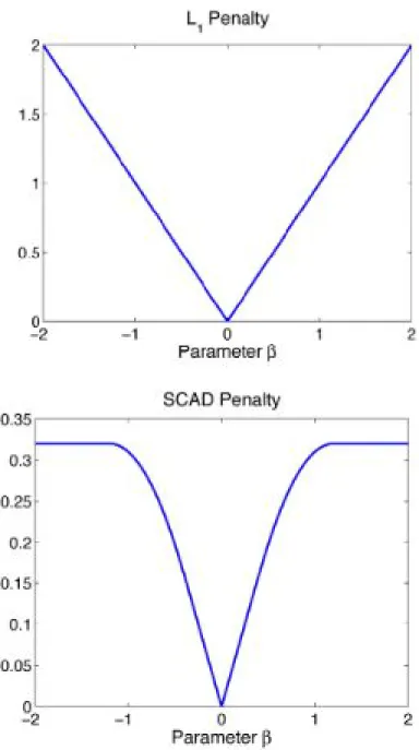
2.1 Penalty Functions and Optimization 21
Figure 2.1 (a) results in sparsity, the LASSO solution is the first place that the contours touch the square and this sometimes occur at a corner corresponding to a zero coefficient. On the contrary, Figure 2.1 (b) depicting ridge regression solution has no corners for the contours to hit hence zero solutions will rarely result.
2.1.2
SCAD
Fan and Li (2001) argued that an ideal penalty function should yield an estimator with the following three properties;
1. Unbiasedness: The estimator is nearly unbiased when the true unknown param-eter is large to reduce model bias.
2. Sparsity: The estimator is a thresholding rule which automatically sets small estimated coefficients to zero to reduce model complexity.
3. Continuity: The estimator is continuous in the data to reduce instability in model prediction.
In contrast, the convex LASSO penalty (L1 penalty) does not satisfy the unbiasedness condition, the convex Lq penalty with q > 1 does not satisfy the sparsity condition
and the concaveLq penalty with 0≤q <1 does not satisfy the continuity condition.
2.1 Penalty Functions and Optimization 22
Smoothly Clipped Absolute Deviation (SCAD) which simultaneously achieves the three desirable properties: unbiasedness, sparsity and continuity. The SCAD penalty function is continuous and the first derivative for some a >2 and β >0 is
p′λ(β) =λ { I(β > λ) + (aλ−β)+ (a−1)λ I(β > λ) } . (2.4)
The SCAD function is given by
pλ(βj) = ⎧ ⎪ ⎪ ⎪ ⎪ ⎪ ⎪ ⎪ ⎪ ⎪ ⎨ ⎪ ⎪ ⎪ ⎪ ⎪ ⎪ ⎪ ⎪ ⎪ ⎩ λ|βj| if |βj| ≤λ − ( |βj|2−2aλ|βj|+λ2 2(a−1) ) if λ <|βj| ≤aλ (a−1)λ2 2 if |βj|> aλ. (2.5)
The SCAD penalty is continuously differentiable on (−∞,0)∪(0,∞), but not differ-entiable at zero. Its derivative vanishes outside [−aλ, aλ]. As a consequence, SCAD penalized regression can produce sparse set of solution and approximately unbiased coefficients for large coefficients.
In Figure 2.2, we sketch the LASSO penalty along with the SCAD. Both penalty functions are equal to zero when the regression coefficient is equal to zero. It is seen that for small values SCAD is similar to the LASSO penalty whereas for larger val-ues SCAD levels off. The SCAD improves the LASSO by reducing the estimation bias. Following Fan and Li (2001), let the parameter vector β be partitioned into
2.1 Penalty Functions and Optimization 23
2.1 Penalty Functions and Optimization 24
givenβ= 0 . Under some regularity conditions, it may be shown that ˆβT = ( ˆβT1,βˆT2) satisfies the oracle properties, since ˆβ2 −→P 0 and ˆβ1 is asymptotic normal with covari-ance matrix J1(β1)−1 if n−1/2λn → ∞. To obtain a penalized maximum likelihood
estimator ofβ, we maximize (2.1) with respect toβ for some thresholding parameter
λ. For computational purposes, Fan and Li (2001) used quadratic functions to locally approximate the penalty function.
2.1.3
Local Quadratic Approximation (LQA)
Algorithm
Suppose we choose an initial valueβ0 near the maximizer of (2.1). If the jth compo-nent ofβ0, βj0 is very close to zero, then set ˆβj0 = 0, otherwise, the penalty Pλ(|βj|)
can be approximated as Pλ(|βj|)≈ Pλ(|βj0|) + 1 2 { Pλ′(|βj0|)/|βj0| } (βj2−βj20),
for βj ≈βj0. In other words,
[Pλ(|βj|)]′ = Pλ′(|βj|)sgn(βj)≈ {Pλ′(|βj0|)/|βj0|}βj, when βj ̸= 0.
This method significantly reduces the computational burden. However, a drawback of this approximation is that once a coefficient is shrunken to zero, it will be excluded from the final selected model. The maximization problem (2.1) can be reduced to a
2.1 Penalty Functions and Optimization 25
quadratic maximization problem assuming that the log-likelihood function is smooth with respect to β so that its first two partial derivatives are continuous. Thus using Taylor expansion, the first term in (2.1) can be locally approximated by
ℓ(β0) +∇ℓ(β0)T(β−β0) + 1 2(β−β0) T∇2ℓ(β 0) T(β−β 0) + 1 2nβ TΣ λ(β0)β (2.6) with ∇ℓ(β0) = ∂ℓ(β0) ∂β ,∇ 2 ℓ(β0) = ∂ 2ℓ(β 0) ∂β∂βT and Σλ(β0) = diag(Pλ′(|β10|)/|β10|, . . . , Pλ′(|βp0|)/|βp0|)
With the aid of this local quadratic approximation, Newton-Raphson (N-R) algorithm can be used to maximize (2.1) iteratively. The estimate ofβˆat the (r+ 1)th iterative step is ˆ βr+1 = ˆβr− { ∇2ℓ(β r)−nΣλ( ˆβr) }−1 { ∇ℓ(βr)−nUλ( ˆβr) } , (2.7)
with Uλ( ˆβr)=Σλ(βr)βr. We iterate this algorithm until convergence.
A perturbed version of the LQA, the Minorization-Maximization (MM) (Hunter and Li (2005)) algorithms have been introduced which alleviates a drawback of backward stepwise variable selection in LQA, but it is difficult to choose the size of perturbation. LQA and MM share the convergence properties of the modified N-R algorithm, using a robust local quadratic approximation. In both cases, the Hessian matrix is guaranteed to be positive definite, driving convergence at least to a local maximum.
2.2 GEE for Mixed Outcomes 26
2.1.4
Standard Error
Fan and Li (2001) recommend estimating the covariance matrix of the non-vanishing (non-zero) component of βˆvia sandwich formula:
ˆ cov(βˆ) =[∇2ℓ(βˆ)−nΣ λ( ˆβ) ]−1 ˆ cov{∇ℓ(βˆ)}[∇2ℓ(βˆ)−nΣ λ( ˆβ) ]−1 . (2.8)
Fan and Li (2001) showed that the LASSO penalty proposed by Tibshirani (1996) has good performance when the signal to noise ratio is large, but creates excessive biases compared to using the SCAD penalty.
2.2
GEE for Mixed Outcomes
In a longitudinal study of n subjects, if the investigators are mainly interested in the covariate effect on the response variable, Liang and Zeger (1986) proposed the GEE model based on the marginal distributions of the response. In a cross-sectional study with multiple responses, Coffey and Gennings (2007a) used GEE approach to estimate the parameters. Let the observations (ymi , xmi ) denote the response and covariate re-spectively for themth response (m = 1,2, . . . , Mi ) measured on subject i= 1, . . . , n.
The Mi×1 vector of responses for the ith subject is y= (y
(1) i , y (2) i , ..., y (Mi) i ).
To apply quasi-likelihood method to the analysis, we define the first two moments of y(im);
2.2 GEE for Mixed Outcomes 27
E(y(im)) = µi(m) =f(xmi ,β(m)), var(yi(m)) =s(m)h(m)(µ(im)) =σi2(m),
whereh(m)(·) is a known function,s(m) is a scaling parameter,f(m)(·) is the nonlinear function of the coefficients and β(m) is a p(m) × 1 vector of model coefficients for the mth response variable. Let β = (β(1)T,β(2)T, . . . ,β(M)T)T be the p×1 vector of model parameters for all M outcomes, wherep= (p(1)+p(2)+· · ·+p(M)). In the quasi - likelihood framework with multiple outcomes, the regression coefficients β can be estimated by solving the Generalized Estimating Equations (GEEs)
S(β)=
n
∑
i=1
DTi Vi−1ri =0. (2.9)
For each subject i, let
Di = ⎛ ⎜ ⎜ ⎜ ⎜ ⎜ ⎜ ⎜ ⎜ ⎜ ⎜ ⎜ ⎜ ⎝ ∂µ(im) ∂β(1)T 0 T · · · 0T 0T ∂µ (m) i ∂β(2)T · · · 0 T .. . ... . .. ... 0T 0T · · · ∂µ (m) i ∂β(Mi)T ⎞ ⎟ ⎟ ⎟ ⎟ ⎟ ⎟ ⎟ ⎟ ⎟ ⎟ ⎟ ⎟ ⎠ ,
2.3 Variable Selection via Penalized GEE 28
and Vi = A
1/2
i Ri(α)A
1/2
i , the Mi ×Mi working covariance matrix of yi. Here, Ai
= diag(σ2(1)i , σ2(2)i , . . . , σ2(Mi)
i ) is aMi×Mi diagonal matrix of var(y
(m)
i ) andRi(α)is
a Mi×Mi working correlation matrix parameterized with parameter vector α. The
GEE estimatorβˆis asymptotically consistent as n goes to infinity. In the presence of high dimensional covariates we extend (2.9) to penalized estimating equations. Thus a penalty term can be incorporated with the aim of adjusting the model to facilitate the estimation of unbiased parameter estimates.
2.3
Variable Selection via Penalized GEE
Fu (2003) proposed a generalization of the bridge and LASSO penalties to GEE models, which minimizes the penalized deviance criterion
D(β;X, y) +P(β), (2.10)
where D(β;X, y) = 2ℓ(y;y) −2ℓ(µ;y) (McCullagh and Nelder, 1989) with log-likelihood ℓ(µ;y) and P(β) = λ∑
j
|βj|q, given q > 0. The LASSO estimator is
defined to be a special case with q = 1 (Tibshirani, 1996). This leads to solving penalized equations;
2.3 Variable Selection via Penalized GEE 29 ⎧ ⎪ ⎪ ⎪ ⎪ ⎪ ⎪ ⎪ ⎪ ⎨ ⎪ ⎪ ⎪ ⎪ ⎪ ⎪ ⎪ ⎪ ⎩ F1(β, X, y) + ˙P1 = 0 . . . Fp(β, X, y) + ˙Pp = 0 , (2.11)
where Fj(β, X, y) is the jth score of the likelihood and ˙Pj =λ
∑
j
q|βj|q−1sgn(|βj|).
This could be generalized to GEE quasi-score function equations.
n
∑
i=1
DiTVi−1ri−nP˙λ(β)=0, (2.12)
where ˙Pλ(β) =∂Pλ(β)/∂βis the vector derivative of the penalty function. Fu (2003)
proposed a method by adjusting the iteratively reweighted least squares method for the penalty function which is equivalent to LQA algorithm. Dziak and Li (2006) proposed using SCAD for GEE models and showed that SCAD may provide bet-ter estimation and selection performance than LASSO. Although different penalty functions can be adopted, in this research we consider only two important penalty functions: LASSO and SCAD. The first possesses the sparsity function and the second simultaneously achieves the three desirable properties of variable selection: sparsity, unbiasedness and continuity, Fan and Li (2001).
2.3 Variable Selection via Penalized GEE 30
2.3.1
Correlation Structure
An attractive feature of the penalized GEE is that the consistency of the estimated parameters hold even if the working correlation,R(α)is misspecified. There are sev-eral choices for the working correlation structure - independent, exchangeable, and first-order autoregressive (AR(1)) must be specified. However, Sutradhar and Das (1999), Wang and Carey (2003), and Shults et al (2006) showed that an incorrectly specified correlation structure leads to substantial loss in estimation efficiency. The correlation pattern in analyses of different types of responses is rarely known and dif-ficult to specify. Thus, we suggest using unstructured correlation structure, Ru(α)
to prevent misspecification and loss of efficiency. Liang and Zeger (1986) suggested simply using the moment estimators based on Pearson residuals to estimate the corre-lation. LetVˆ(α)= ˆA1/2diag( ˆRu, . . . ,Rˆu) ˆA1/2 be the unstructured covariance matrix
estimate. Specifically, ˆ Ru = 1 n n ∑ i=1 ˆ A−i 1/2ririTAˆ −1/2 i , (2.13)
where ˆRu is obtained without any assumption on the specific structure on the true
2.3 Variable Selection via Penalized GEE 31
2.3.2
Computational Algorithm
To computeβˆ, we use the local quadratic approximation (LQA) algorithm suggested by Fan and Li (2001). With the aid of the LQA, the optimization of (2.12) can be car-ried out using a modified Newton-Raphson (MNR) algorithm. Letβr = (β1r, . . . , βpr)
be the parameter estimate at the rth iteration.
• We start with an initialβ0 ordinary least squares estimate.
• For each iteration r, if βjr is very close to 0 then set ˆβjr = 0.
• Otherwise the penalty can be locally approximated by the quadratic function. The derivative of the penalty can be approximated as
[Pλ(|βj|)]′ = Pλ′(|βj|)sgn(βj)≈ {Pλ′(|βj|)/|βj|}βj.
Thus using Taylor expansions, we can locally approximate equation (2.12) by
S(βr) + ∂S(βr) ∂β (β−βr)−nUλ(βr)−nΣλ(βr)(β−βr) +· · ·= 0 (2.14) where Σλ(βr) = diag(Pλ′(|β1r|)/|β1r|, . . . , Pλ′(|βpr|)/|βpr|), Uλ(βr) = Σλ(βr)βr.
2.3 Variable Selection via Penalized GEE 32
• Applying Newton-Raphson method to equation (2.14), we obtain the follow-ing iteration for solvfollow-ing the penalized generalized estimatfollow-ing equation. The estimate of βˆ in the (r+ 1)th iteration is,
ˆ βr+1 = ˆβr− {∂S(βˆr) ∂β −nΣλ( ˆβr) }−1 { S(βˆr)−nUλ( ˆβr) } . (2.15)
• Given a selected tuning parameter λ, we repeat the above algorithm to update
ˆ
βr until convergence. The convergence criterion is
∥βˆr−βˆr−1∥2 < ϵ. for a pre-specified small constant, ϵ.
2.3.3
Tuning Parameter Selection
The numerical performance and the asymptotic behaviour of the penalized regression models rely on the appropriate choice of the tuning parameter. The tuning parameters are often employed to balance model sparsity and goodness-of-fit. To optimize the thresholding parameters θ = (λ, a) for SCAD, we fix a = 3.7 as suggested by Fan and Li (2001) in practice and only tune λ for SCAD and θ = λ for other penalty functions (LASSO). Here we discuss two methods of estimatingλ: Generalized Cross-Validation (GCV) (Craven and Wahba, 1979) and Bayesian Information Criterion (BIC) (Schwarz, 1978).
2.3 Variable Selection via Penalized GEE 33
Generalized Cross-Validation (GCV)
Generalized Cross-Validation (GCV) proposed by Craven and Wahba (1979) aims to approximate the leave- one-out cross validation criterion. In the GCV approach, the value of λ that achieves the minimum of the GCV is the optimal tuning parameter. The minimization can be carried out by searching over a predetermined grid of points for λ. For linear smoothers (ˆy =Ly), the GCV is defined by
GCV(λ) = 1
n
RSS(β(λ))
(1−n−1df(λ))2, (2.16)
whereRSS(β(λ)) = (y−Xβ)T(y−Xβ) and df(λ) =tr(X(XTX+nΣλ)−1XT) is the
trace of the smoothing matrix L, often called effective number of parameters; Hastie & Tibshirani (1990), Tibshirani (1996) and Fan & Li (2001). The GCV is com-putationally convenient and remains as one popular criterion is selecting smoothing parameter. The nonlinear GCV for the generalized linear model is defined as
GCV(λ) = Dev
n(1−n−1df(λ))2, (2.17)
whereDev= 2ℓ(y, y)−2ℓ(µ, y) is the model deviance (McCullagh and Nelder, 1989). The model deviance replaces the RSS in the GCV for non-Gaussian distributions in the exponential family. Fu (2003) also recommended an adaptation of GCV where
2.3 Variable Selection via Penalized GEE 34
RSS is generalized to the weighted deviance,
W Dev=
n
∑
i=1
rTi R−i 1ri, (2.18)
where ri = (yi−µi) are the deviance residuals and Ri is the working correlation
matrix.
Bayesian Information Criterion(BIC)
In model selection, Wang et al.(2007) showed that the tuning parameter that is se-lected by the BIC can identify the true model consistently. Several researchers use BIC for selecting the optimal λ by minimizing
BIC(λ) = log (RSS(λ) N ) + (log(N) N ) df(λ) (2.19)
wheredf(λ) is estimated as the number of nonzero variables inβˆ(λ) (Zou et al., 2007). The resulting optimal regularization parameter ˆλBIC is then selected as the one that
minimizes the BIC(λ). The BIC criteria can also be extended beyond linear models by replacing RSS(λ) with a weighted sum of squares or model deviance (Poisson, binomial, etc).
2.3 Variable Selection via Penalized GEE 35
2.3.4
Asymptotic Properties
In this section, we discuss the asymptotic properties for penalized GEE estimator as the number of subjects goes to infinity. Let
S(β)= n ∑ i=1 DiTVi−1ri, (2.20) K(β)= 1 n n ∑ i=1 DiTVi−1Di, (2.21)
where Vi is the working covariance and is not assumed to be the same as the true
covariance. For analysis of longitudinal data using penalized estimating equations, Dziak (2006) showed that the asymptotic consistency and normality of ˆβ depends on the following regularity conditions:
(1) S(β)and K(β) have continuous third derivative in β.
(2) K(β)is positive definite with probability approaching one andthere exist a non-random functionK0(β) such that∥K(β)−K0(β)∥
p − →0 uniformly,K0(β)>0 for all β. (3) Si = ∑ i=1
DTi Vi−1ri have finite covariance for all β.
(4) The derivative ofK0(β) in β are Op(n−1/2) for all β.
Liang and Zeger (1986) proposed GEEs for the analysis of longitudinal data with a generalized linear model. The GEEs are multivariate extensions of quasi-likelihood.
2.3 Variable Selection via Penalized GEE 36
Modeling the same way as longitudinal data, the following theorems from Dziak (2006) can be easily extended to apply to GEE for the multivariate multiple regression case. Assumingµ(im) is correctly specified byf(m)(x(im),β(m)), ˆαand scaling parameters are appropriately chosen, then smooth nonlinear models with continuous derivatives have been shown to satisfy these regularity conditions for penalized estimating equation with multiple outcomes. Dziak (2006) states the following theorems;
Theorem 2.1. Under regularity conditions (1)−(4), for LASSO with λ=Op(n−1/2)
or for SCAD penalty with λ =op(1) there exists a sequence βˆn of solutions such that
∥βˆn−β∥=Op(n−1/2).
Following Dziak (2006), Theorem 2.1 shows model consistency of the penalized estimating equation 2.12 with LASSO (λ = Op(n−1/2)) and SCAD penalty ( λ =
op(1)) when the number of subjects n goes to infinity. If β = (βA,βN) is the true
vector of regression coefficients with two subsets: A = {j : βj ̸= 0} as the active
(non-zero) coefficients and N = {j : βj = 0} as the inactive (zero) coefficients then
for selection consistency, we require both sparsity (deleting zero coefficients) and sensitivity (retaining non-zero coefficients) properties (Fan and Li, 2001).
2.3 Variable Selection via Penalized GEE 37
there exist a sequence βˆ of solutions to equation 2.12 such that √
n(βˆA−βA)
L
−
→N(0,Φ) (2.22)
Again, following Dziak (2006) Theorem 2.2 indicates that the parameter estimates for 2.12 are asymptotically normal, i.e,
√
n(βˆ−β)→−L N(0,Φ) (2.23)
where Φis the limit in probability of
Φn= [∑n i=1 DiTVi−1Di−nΣλ( ˆβ) ]−1{∑n i=1 DiTVi−1cov(yi)Vi−1Di }[∑n i=1 DiTVi−1Di−nΣλ( ˆβ) ]−1
Since the proofs of Theorem 2.1 and 2.2 are similar to that of Dziak (2006) by replacing quasi-likelihood based on multiple responses (Coffey and Gennings, 2007a, 2007b), we ignore the proofs here.
It should be noted that the variable selection methods in general does not guaran-tee the consistency property there by does not guaranguaran-tee classical inference theory in some situations. Post-selection inference procedure is one of the option to overcome the problem by utilizing the cross-validation approach to part of the data.
Chapter 3
Simulation Studies
We conducted a series of simulation studies to investigate the performance of our proposed variable selection approach on continuous, binary and count response out-comes using the LASSO and SCAD penalty functions. Simulations were conducted using the R software. For faster computations in optimization of tuning parameter
λ, we used the “warm-starting” principle, where the initial value of β is replaced by βˆ(λ+δλ) for the modified N-R algorithm in each simulation. The model that has minimum BIC(λ) or GCV(λ) is identified as the best model. The model performance is assessed using model error (ME, Fan and Li 2001) and their standard error, correct deletions and incorrect deletions. Model error is due to lack of fit of an underlying model and is denoted by M E( ˆβ). The size of the model error reflects how well the
Simulation Studies 39
model fits the data.
M E( ˆβ) = Ex{µ(Xβ)−µ(Xβ)}ˆ 2
where µ(Xβ)=E(y|X). Model error has been expressed as median of the relative model error (MRME). The relative model error is defined as
RM E = M E
M Ef ull
,
where M Ef ull is the model error calculated by fitting the data with the full model.
Correct deletions are the average number of true zero coefficients correctly estimated as zero and incorrect deletions are the average number of true nonzero coefficients erroneously set to zero. Estimated values for correct and incorrect deletions are reported in the columns “Correct” and “Incorrect”, respectively. For comparison purposes, we estimated the covariance matrix of the response variables based on both unstructured working correlation (UWC) and independent working correlation (IWC) to investigate the performance of the GEE methodology (Coffey & Gennings, 2007a). We simulated 1000 data sets consisting of n= 50 and n = 100 observations from the response model
g(E(Y)) = XijTβ
where i = 1,2, . . . n subjects and j = 1,2, . . . , m responses. For binary outcomes we use a logit link, log link for count and for a continuous (normal) outcome we use
3.1 Simulation for Normal and Binary responses 40
the identity link function. The covariates Xij were generated from the multivariate
normal distribution with marginal mean 0, marginal variance 1 and AR(1) correla-tion with ρx = 0.5. For simulations, we considered the following cases of continuous,
binary and count response outcomes with different trueβ values and correlation pa-rameter, ρy between the responses and σ2y = 1.
3.1
Simulation for Normal and Binary responses
3.1.1
Case 1: Correlated Three Normal Responses
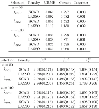
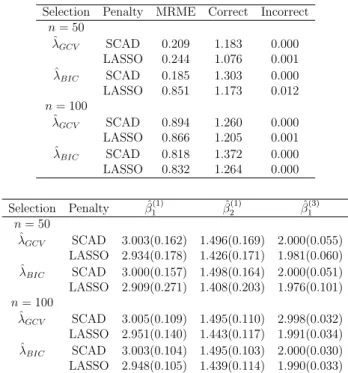
We consider correlated normal responses (m = 3) with AR(1) true correlation with pa-rameterρy = 0.7 and two covariates (k = 2) withβ = (β(1),β(2),β(3)) = ((3,1.5),(0,0),
(2,0)). Simulation results are summarized in Tables 3.1 and 3.2 for IWC and UWC respectively. From Table 3.1 & 3.2, we see that the nonzero estimates of both SCAD and LASSO are close to the true values, i.e: β1(1) = 3, β2(1) = 1.5 and β1(3) = 2 but the standard errors of the estimates in Table 3.2 decreases which can be attributed to the correlation between the responses. For both n = 50 and n = 100, the mean model error and its standard error for SCAD are smaller than LASSO. The average number of zero coefficients increases asn increases in Table 3.2 especially for SCAD.
3.1 Simulation for Normal and Binary responses 41
Selection Penalty MRME Correct Incorrect
n= 50 ˆ λGCV SCAD 0.064 1.297 0.000 LASSO 0.092 0.982 0.001 ˆ λBIC SCAD 0.053 1.532 0.000 LASSO 0.113 1.180 0.002 n= 100 ˆ λGCV SCAD 0.030 1.298 0.000 LASSO 0.038 0.871 0.001 ˆ λBIC SCAD 0.025 1.538 0.000 LASSO 0.043 1.066 0.000 Selection Penalty βˆ1(1) βˆ (1) 2 βˆ (3) 1 n= 50 ˆ λGCV SCAD 2.998(0.171) 1.496(0.168) 1.993(0.154) LASSO 2.898(0.203) 1.388(0.219) 1.831(0.229) ˆ λBIC SCAD 2.998(0.171) 1.496(0.168) 1.992(0.147) LASSO 2.866(0.236) 1.356(0.244) 1.789(0.266) n= 100 ˆ λGCV SCAD 2.998(0.115) 1.506(0.116) 1.996(0.105) LASSO 2.931(0.170) 1.438(0.154) 1.891(0.152) ˆ λBIC SCAD 2.998(0.115) 1.506(0.115) 1.998(0.100) LASSO 2.898(0.216) 1.403(0.192) 1.857(0.190)
Table 3.1: Simulations results for correlated normal responses (Case 1) with IWC.
This indicates that SCAD performs well compared to LASSO.
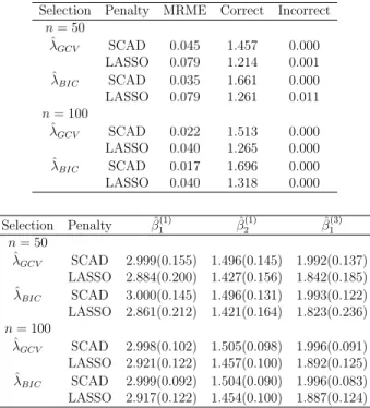
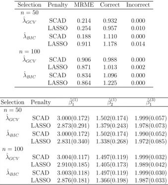
3.1.2
Case 2: Correlated Two Normal and One Independent
Binary Responses
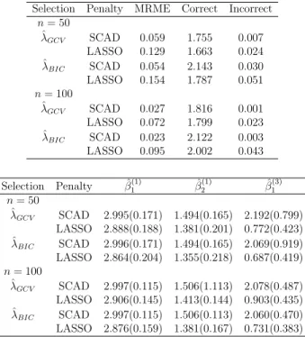
We simulated three outcomes (m= 3) - two continuous and one binary. The contin-uous outcomes were generated from a normal distribution and were correlated with AR(1) true correlation with parameterρy = 0.7 and the binary outcome from an
3.1 Simulation for Normal and Binary responses 42
Selection Penalty MRME Correct Incorrect
n= 50 ˆ λGCV SCAD 0.045 1.457 0.000 LASSO 0.079 1.214 0.001 ˆ λBIC SCAD 0.035 1.661 0.000 LASSO 0.079 1.261 0.011 n= 100 ˆ λGCV SCAD 0.022 1.513 0.000 LASSO 0.040 1.265 0.000 ˆ λBIC SCAD 0.017 1.696 0.000 LASSO 0.040 1.318 0.000 Selection Penalty βˆ1(1) βˆ (1) 2 βˆ (3) 1 n= 50 ˆ λGCV SCAD 2.999(0.155) 1.496(0.145) 1.992(0.137) LASSO 2.884(0.200) 1.427(0.156) 1.842(0.185) ˆ λBIC SCAD 3.000(0.145) 1.496(0.131) 1.993(0.122) LASSO 2.861(0.212) 1.421(0.164) 1.823(0.236) n= 100 ˆ λGCV SCAD 2.998(0.102) 1.505(0.098) 1.996(0.091) LASSO 2.921(0.122) 1.457(0.100) 1.892(0.125) ˆ λBIC SCAD 2.999(0.092) 1.504(0.090) 1.996(0.083) LASSO 2.917(0.122) 1.454(0.100) 1.887(0.124)
Table 3.2: Simulations results for correlated normal responses (Case 1) with UWC.
((3,1.5),(0,0),(2,0)). Simulation results are summarized in Tables 3.3 and 3.4 for IWC and UWC respectively. We see from Tables 3.3 & 3.4 that, the nonzero estimates for IWC remained similar to those in UWC. However because of the large correlation (0.7) between the continuous responses, the standard errors of β1(1) = 3,
β2(1) = 1.5 decreases for UWC. Again, the average number of zero coefficients increases for UWC compared to IWC. As the sample size of SCAD is increased, the mean model error and its standard error decreases for both GCV and BIC. LASSO estimates for
3.1 Simulation for Normal and Binary responses 43
Selection Penalty MRME Correct Incorrect
n= 50 ˆ λGCV SCAD 0.059 1.755 0.007 LASSO 0.129 1.663 0.024 ˆ λBIC SCAD 0.054 2.143 0.030 LASSO 0.154 1.787 0.051 n= 100 ˆ λGCV SCAD 0.027 1.816 0.001 LASSO 0.072 1.799 0.023 ˆ λBIC SCAD 0.023 2.122 0.003 LASSO 0.095 2.002 0.043 Selection Penalty βˆ1(1) βˆ (1) 2 βˆ (3) 1 n= 50 ˆ λGCV SCAD 2.995(0.171) 1.494(0.165) 2.192(0.799) LASSO 2.888(0.188) 1.381(0.201) 0.772(0.423) ˆ λBIC SCAD 2.996(0.171) 1.494(0.165) 2.069(0.919) LASSO 2.864(0.204) 1.355(0.218) 0.687(0.419) n= 100 ˆ λGCV SCAD 2.997(0.115) 1.506(1.113) 2.078(0.487) LASSO 2.906(0.145) 1.413(0.144) 0.903(0.435) ˆ λBIC SCAD 2.997(0.115) 1.506(0.113) 2.060(0.470) LASSO 2.876(0.159) 1.381(0.167) 0.731(0.383)
Table 3.3: Simulations results for correlated normal and independent binary responses (Case 2) with IWC.
close to the true values for SCAD. Thus, SCAD performs well compared to LASSO.
3.1.3
Case 3 : Correlated Two Normal and One Binary
Re-sponses
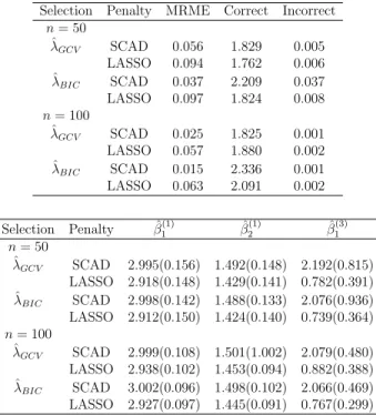
We simulated three outcomes (m= 3) - two continuous and one binary generated us-ing unstructured correlation structure with parametersρ12 = 0.3, ρ13= 0.4 andρ23= 0.6 and two covariates (k= 2) withβ= (β(1),β(2),β(3)) = ((3,1.5),(0,0),(2/3,0)).The
3.1 Simulation for Normal and Binary responses 44
Selection Penalty MRME Correct Incorrect
n= 50 ˆ λGCV SCAD 0.056 1.829 0.005 LASSO 0.094 1.762 0.006 ˆ λBIC SCAD 0.037 2.209 0.037 LASSO 0.097 1.824 0.008 n= 100 ˆ λGCV SCAD 0.025 1.825 0.001 LASSO 0.057 1.880 0.002 ˆ λBIC SCAD 0.015 2.336 0.001 LASSO 0.063 2.091 0.002 Selection Penalty βˆ1(1) βˆ (1) 2 βˆ (3) 1 n= 50 ˆ λGCV SCAD 2.995(0.156) 1.492(0.148) 2.192(0.815) LASSO 2.918(0.148) 1.429(0.141) 0.782(0.391) ˆ λBIC SCAD 2.998(0.142) 1.488(0.133) 2.076(0.936) LASSO 2.912(0.150) 1.424(0.140) 0.739(0.364) n= 100 ˆ λGCV SCAD 2.999(0.108) 1.501(1.002) 2.079(0.480) LASSO 2.938(0.102) 1.453(0.094) 0.882(0.388) ˆ λBIC SCAD 3.002(0.096) 1.498(0.102) 2.066(0.469) LASSO 2.927(0.097) 1.445(0.091) 0.767(0.299)
Table 3.4: Simulations results for correlated normal and independent binary responses (Case 2) with UWC.
instability. Correlated normal and binary outcomes were generated in R using the
BinNorpackage of Anup Amatya and Hakan Demirtas for generating multiple binary and normal variables simultaneously given marginal characteristics and association structure based on the methodology proposed by Demirtas and Doganay (2012). Sim-ulation results are summarized in Tables 3.5 and 3.6 for IWC and UWC respectively. From Tables 3.5 & 3.6., we see that if the sample size is increased, the mean model error and its standard error are reduced. Again, the standard error of the nonzero parameter estimates for UWC are reduced compared to IWC. The average number of
3.1 Simulation for Normal and Binary responses 45
Selection Penalty MRME Correct Incorrect
n= 50 ˆ λGCV SCAD 0.071 1.916 0.209 LASSO 0.092 1.343 0.173 ˆ λBIC SCAD 0.070 2.446 0.301 LASSO 0.119 1.509 0.258 n= 100 ˆ λGCV SCAD 0.034 1.775 0.066 LASSO 0.050 1.449 0.084 ˆ λBIC SCAD 0.047 2.430 0.151 LASSO 0.056 1.622 0.152 Selection Penalty βˆ1(1) βˆ (1) 2 βˆ (3) 1 n= 50 ˆ λGCV SCAD 2.997(0.167) 1.499(0.171) 0.543(0.520) LASSO 2.899(0.202) 1.395(0.214) 0.241(0.224) ˆ λBIC SCAD 2.997(0.167) 1.499(0.170) 0.246(0.461) LASSO 2.886(0.219) 1.361(0.238) 0.212(0.222) n= 100 ˆ λGCV SCAD 2.998(0.114) 1.503(0.116) 0.633(0.201) LASSO 2.918(0.149) 1.421(0.157) 0.287(0.194) ˆ λBIC SCAD 2.998(0.113) 1.503(0.115) 0.309(0.432) LASSO 2.892(0.166) 1.393(0.188) 0.253(0.185)
Table 3.5: Simulations results for correlated normal and binary responses (Case 3) with IWC.
zero coefficients using SCAD with BIC for all sample size are close the target value of three and the nonzero estimated coefficients are close to the true values forn = 50 and n = 100 for SCAD with GCV.
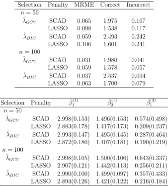
3.1.4
Case 4 : Correlated Two Normal and One Independent
Count Responses
We simulated three outcomes (m = 3) - two continuous and one count. The contin-uous outcomes were generated from a normal distribution and were correlated with
3.1 Simulation for Normal and Binary responses 46
Selection Penalty MRME Correct Incorrect
n= 50 ˆ λGCV SCAD 0.065 1.975 0.167 LASSO 0.098 1.538 0.117 ˆ λBIC SCAD 0.059 2.493 0.242 LASSO 0.106 1.601 0.241 n= 100 ˆ λGCV SCAD 0.031 1.980 0.041 LASSO 0.059 1.578 0.057 ˆ λBIC SCAD 0.037 2.537 0.094 LASSO 0.063 1.700 0.079 Selection Penalty βˆ1(1) βˆ (1) 2 βˆ (3) 1 n= 50 ˆ λGCV SCAD 2.998(0.153) 1.496(0.153) 0.574(0.498) LASSO 2.883(0.178) 1.417(0.173) 0.209(0.237) ˆ λBIC SCAD 2.993(0.147) 1.495(0.145) 0.287(0.464) LASSO 2.872(0.180) 1.407(0.181) 0.190(0.219) n= 100 ˆ λGCV SCAD 2.998(0.105) 1.500(0.106) 0.643(0.337) LASSO 2.907(0.121) 1.442(0.113) 0.256(0.211) ˆ λBIC SCAD 2.990(0.100) 1.499(0.097) 0.357(0.433) LASSO 2.894(0.126) 1.421(0.122) 0.216(0.184)
Table 3.6: Simulations results for correlated normal and binary responses (Case 3) with UWC.
AR(1) true correlation with parameterρy = 0.7 and the count outcome from an
inde-pendent Poisson observations and two covariates (k = 2) withβ= (β(1),β(2),β(3)) = ((3,1.5),(0,0),(2,0)). Simulation results are summarized in Table 3.7 and 3.8 for IWC and UWC respectively. From Tables 3.7 & 3.8., we see that the nonzero parameter estimates are close to the true values. The incorporation of the correlation resulted in decreased standard errors of nonzero parameters.
Overall, from Tables 3.1-3.8, we see that the nonzero estimates are unbiased re-gardless of the correlation structure. However the unstructured correlation resulted in
3.1 Simulation for Normal and Binary responses 47
Selection Penalty MRME Correct Incorrect
n= 50 ˆ λGCV SCAD 0.214 0.932 0.000 LASSO 0.254 0.957 0.010 ˆ λBIC SCAD 0.188 1.110 0.000 LASSO 0.911 1.178 0.014 n= 100 ˆ λGCV SCAD 0.906 0.988 0.000 LASSO 0.871 1.013 0.002 ˆ λBIC SCAD 0.834 1.096 0.000 LASSO 0.864 1.225 0.000 Selection Penalty βˆ1(1) βˆ (1) 2 βˆ (3) 1 n= 50 ˆ λGCV SCAD 3.000(0.172) 1.502(0.174) 1.999(0.057) LASSO 2.873(0.291) 1.379(0.243) 1.978(0.073) ˆ λBIC SCAD 3.000(0.172) 1.502(0.174) 1.990(0.052) LASSO 2.831(0.340) 1.338(0.268) 1.972(0.085) n= 100 ˆ λGCV SCAD 3.004(0.117) 1.497(0.119) 1.999(0.032) LASSO 2.910(0.185) 1.405(0.173) 1.989(0.042) ˆ λBIC SCAD 3.003(0.118) 1.497(0.119) 1.999(0.030) LASSO 2.876(0.181) 1.366(0.198) 1.987(0.033)
Table 3.7: Simulations results for correlated normal and independent count responses (Case 4) with IWC.
decreased standard errors of estimates compared to independent working correlation based estimates. The average number of zero coefficients increases in unstructured correlation tables compared to independent. We notice a decrease in mean model error when the sample size increases from 50 to 100 for both LASSO and SCAD. SCAD has smaller mean model error than LASSO in all cases. Specifically, SCAD with BIC perform well.
3.1 Simulation for Normal and Binary responses 48
Selection Penalty MRME Correct Incorrect
n= 50 ˆ λGCV SCAD 0.209 1.183 0.000 LASSO 0.244 1.076 0.001 ˆ λBIC SCAD 0.185 1.303 0.000 LASSO 0.851 1.173 0.012 n= 100 ˆ λGCV SCAD 0.894 1.260 0.000 LASSO 0.866 1.205 0.001 ˆ λBIC SCAD 0.818 1.372 0.000 LASSO 0.832 1.264 0.000 Selection Penalty βˆ1(1) βˆ (1) 2 βˆ (3) 1 n= 50 ˆ λGCV SCAD 3.003(0.162) 1.496(0.169) 2.000(0.055) LASSO 2.934(0.178) 1.426(0.171) 1.981(0.060) ˆ λBIC SCAD 3.000(0.157) 1.498(0.164) 2.000(0.051) LASSO 2.909(0.271) 1.408(0.203) 1.976(0.101) n= 100 ˆ λGCV SCAD 3.005(0.109) 1.495(0.110) 2.998(0.032) LASSO 2.951(0.140) 1.443(0.117) 1.991(0.034) ˆ λBIC SCAD 3.003(0.104) 1.495(0.103) 2.000(0.030) LASSO 2.948(0.105) 1.439(0.114) 1.990(0.033)
Table 3.8: Simulations results for correlated normal and independent count responses (Case 4) with UWC.
Chapter 4
Case Studies
4.1
Concrete Slump Test Data
In this section, we apply variable selection to concrete slump test data set. The data comes from a study by Yeh, I-Cheng (2006, 2007, 2008, 2009) to model the slump-flow of fly ash and slag concrete as a function of seven concrete ingredients measured in kg/m3, including cement (X1), fly ash (X2), blast furnace slag (X3), water (X4), superplasticizer (X5), and coarse aggregate (X6) and fine aggregate (X7). The data set report some results about two kinds of tests executed on concrete. Concrete is a highly complex material, which makes modeling its behavior a very difficult task. The workability of concrete can be measured by the “concrete slump test”, a simplistic
4.1 Concrete Slump Test Data 50
measure of the plasticity of a fresh batch of concrete. The concrete slump test is in essence, a method of quality control. For a particular mix, the slump should be consis-tent. A change in slump height would demonstrate an undesired change in the ratio of the concrete ingredients; the proportions of the ingredients are then adjusted to keep a concrete batch consistent. This homogeneity improves the quality and structural integrity of the concrete. The second test considered is “compressive strength test” where this test measure the capacity of a material to withstand axially directed push-ing forces. The variance of slump and flow was observed. The slump is the difference of height of the concrete mix after being placed in the slump cone and the cone. It differs from one sample to another. Samples with lower heights are predominantly used in construction, with samples having high slumps commonly used to construct roadway pavements. The flowability is measured in terms of spread, hence the flow correspond to the width of the patty. The three output variables include slump (cm), flow (cm) and 28-day compressive strength (CS) (Mpa). The data comprises 103 samples and it is available athttp://archive.ics.uci.edu/ml/datasets/Concrete+Slump+Test. A more detailed description of the data set can be found in Yeh, I-Cheng (2006, 2007, 2008, 2009). Figure 4.1 and Table 4.1 show the association strength among the three responses. It is shown that slump (Y1) and flow (Y2) are highly correlated, with a positive correlation of 0.9061. We can use penalized GEE to utilize that additional
4.1 Concrete Slump Test Data 51
Figure 4.1: Scatter plot demonstrating visually the relationship between slump (Y1), flow (Y2) and compressive strength (CS) (Y3)
SLUMP FLOW CS
SLUMP 1 0.9061 -0.2233
FLOW 0.9061 1 -0.1240
CS -0.2233 -0.1240 1
Table 4.1: Correlation matrix for the responses
information in the selection of significant variables for this data set. The estimates are given in Table 4.2-4.4.
The second and third columns of Tables 4.2-4.4 represent performance using pe-nalized GEE with IWC for SCAD and LASSO. The fourth and fifth columns of the
4.1 Concrete Slump Test Data 52
IWC UWC
Variable SCAD LASSO SCAD LASSO
X1 – – – – – – – – X2 -0.0297 -0.0375 – – (0.0021) (0.0013) – – X3 -0.0061 -0.0098 -0.0023 -0.0023 (0.0001) (0.0010) (0.0003) (0.0003) X4 0.0866 0.1222 0.0278 0.0278 (0.0003) (0.0025) (0.0015) (0.0015) X5 – – – – – – – – X6 -0.0011 -0.0017 – – (0.0000) (0.000) – – X7 0.0070 – 0.0163 0.0163 (0.0000) – (0.0000) (0.0000)
Table 4.2: Estimates of regression coefficients for slump (Y1), with standard error in parentheses
tables represent performance using penalized GEE with UWC. For the model selec-tion procedures, both unweighted BIC and GCV were used to estimate regression coefficients. However, their performance was similar. Therefore, we present only the results based on the unweighted BIC for both SCAD and LASSO. We see from Ta-ble 4.2 that, SCAD with IWC identified 5 out of the 7 covariates as important for slump(Y1) whereas LASSO with IWC identified 4 covariates. The difference between them is that SCAD kept fine aggregate (X7). SCAD and LASSO with UWC obtained the same estimates for all variables, they retained fine aggregate (X7) but forced fly
4.1 Concrete Slump Test Data 53
IWC UWC
Variable SCAD LASSO SCAD LASSO
X1 – – – – – – – – X2 -0.0529 -0.0715 -0.0169 -0.0169 (0.0024) (0.2544) (0.0022) (0.0022) X3 – – – – – – – – X4 0.2868 0.3341 0.2507 0.2507 (0.0004) (0.0077) (0.0000) (0.0000) X5 – – – – – – – – X6 -0.0033 -0.0121 – – (0.0000) (0.0031) – – X7 – – – – – – – –
Table 4.3: Estimates of regression coefficients for flow (Y2), with standard error in parentheses
ash (X2) and coarse aggregate (X6) to zero. From Table 4.3 we see that, both SCAD and LASSO with IWC chose fly ash (X2), water (X4) and coarse aggregate (X6) as significant ingredients for flow (Y2) but SCAD and LASSO with UWC identified only fly ash (X2) and water (X4) as significant variables. The standard errors of estimates with UWC decreases. From Table 4.4 we see that, LASSO with IWC chose all co-variates as important ingredients for CS (Y3) except coarse aggregate (X6) whereas the others dropped coarse aggregate (X6) as well as superplasticizer (X5).
4.1 Concrete Slump Test Data 54
IWC UWC
Variable SCAD LASSO SCAD LASSO
X1 0.1017 0.1032 0.0972 0.0972 (0.0000) (0.0000) (0.0000) (0.0000) X2 0.0322 0.0337 0.0229 0.0299 (0.0000) (0.0000) (0.0000) (0.0000) X3 0.0920 0.0931 0.0871 0.0871 (0.0004) (0.0003) (0.0007) (0.0007) X4 -0.0866 -0.0802 -0.0494 -0.0494 (0.0000) (0.0000) (0.0000) (0.0000) X5 – 0.0173 – – – (0.0000) – – X6 – – – – – – – – X7 0.0165 0.0174 0.0119 0.0119 (0.0000) (0.0000) (0.0000) (0.0000)
Table 4.4: Estimates of regression coefficients for compressive strength (Y3), with standard error in parentheses
4.1.1
Concrete Slump Test Data With Artificial Binary
Re-sponse
For illustration purposes, we create an artificial binary response variable to indicate whether a specimen can sustain a heavy load before distortion. For this analysis, we consider that concrete with compressive strength less than 35 is of poor quality. So for illustration purpose, we convert this continuous variable response to binary based on the quality. Let Y3 = 1 if the compressive strength is more than 35, and