Multi-objective and semi-supervised heterogeneous classifier ensembles.

(1)

Multi-objective and

Semi-supervised Heterogeneous

Classifier Ensembles

Shenkai Gu

Submitted for the Degree of

Doctor of Philosophy

from the

University of Surrey

Department of Computer Science

Faculty of Engineering and Physical Sciences

University of Surrey

Guildford, Surrey, GU2 7XH, U.K.

April 2016

c

(2)

(3)

Abstract

In the recent years, many applications in machine learning involve an increasingly large number of features and samples, which poses new challenges to many learn-ing algorithms. To address these challenges, ensemble learnlearn-ing methods, which uses multiple base learners, have been proposed to achieve better predictive per-formance.

This thesis covers a range of topics in ensemble classification, including multi-objective and semi-supervised heterogeneous classier ensembles. We first present an empirical study on heterogeneous classifier ensembles, which confirms that het-erogeneous ensembles outperform homogeneous ones and single classifiers. Sec-ondly, we present a multi-objective ensemble generation method, which creates a group of members so that the diversity among the base learners could be ex-plicitly maintained. The third topic of this thesis is a feature selection method for data that has a large number of features. By using the modified competitive swarm optimizer as the search algorithm, we are able to considerably reduce the number of features and at the same time improve the classifiers’ generalisation

(4)

performance. Finally, we present a novel semi-supervised ensemble learning al-gorithm, termed Multi-Train, that uses semi-supervised learning algorithms to learn from unlabelled data.

(5)

Acknowledgements

I am heartily thankful to my supervisor, Prof Yaochu Jin, for his constant support and guidance during my study. His academic knowledge and personal character-istics deeply impressed me and kept encouraging me to move forward. I would also like to thank my co-supervisor, Dr Norman Poh, and Dr Saied Sanei, for their gorgeous ideas and invaluable help.

I would also like to extend my gratitude to the Department of Computer Science, Faculty of Engineering and Physical Science (FEPS), University of Surrey for the financial support to make this research possible.

My thanks and gratitude also goes out to academic visitor Prof Xiaoyan Sun and Prof Chaoli Sun, colleague Dr Yun Yang, Dr Hui Wang, Ran Cheng and everyone in the department. Their kind support, discussions, and feedback are hugely appreciated.

Finally, I would like to send my deepest appreciation to all my parents and friends for their endless love and encouragement that have supported me on a more general level throughout my entire academic studies.

(6)

(7)

List of Figures

2.1 Illustration of Pareto optimal solutions of an MOP denoted by

black dots, where solution A is known as a knee point. . . 23

2.2 Illustration of supervised vs semi-supervised learning [111]. . . 32

3.1 Diagram of an EEG-based motor imaginary detection . . . 43

3.2 Structure of heterogeneous ensembles with same feature . . . 44

3.3 Structure of heterogeneous ensembles with different features . . . 44

4.1 The hypervolume averaged over the six test cases for the six ex-perimental setups. . . 61

4.2 Comparison of single classifier and ensemble classifiers . . . 63

4.3 Pareto fronts achieved in the 36 different setups. . . 64

4.4 Zoomed-in version of representative plots in Fig. 4.3 . . . 65

(14)

5.2 Number of new solutions found in each generation. . . 83 5.3 Average number of selected features over generations. . . 86 5.4 Graphics showing that the selected features (x-axes) of the best

individual over generations (y-axes). The darkness of each pixel represents the frequency of the corresponding feature that has been selected in the respective generation across different experiments -a d-arker colour represents -a higher frequency -and vice vers-a. . . . 87

(15)

List of Tables

2.1 Coincident errors between a pair of classifiers . . . 13

2.2 Range and maximum diversity criteria of measures . . . 16

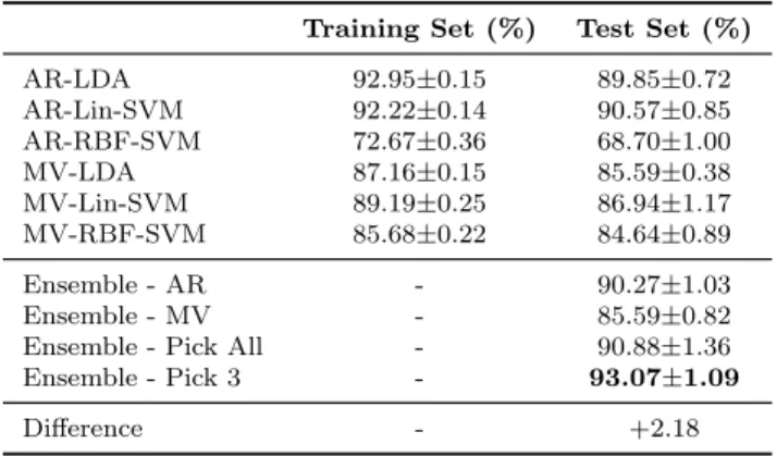
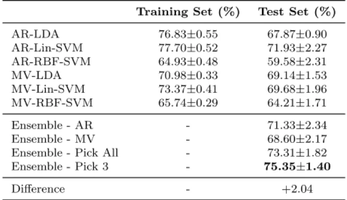
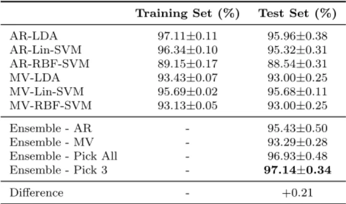
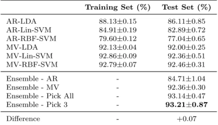
3.1 10-fold on training set - dataset aa . . . 47

3.2 10-fold on training set - dataset al . . . 47

3.3 10-fold on training set - dataset av . . . 48

3.4 10-fold on training set - dataset aw . . . 48

3.5 10-fold on training set - dataset ay . . . 48

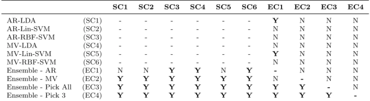
3.6 ‘Pick All’ and ‘Pick 3’ heterogeneous ensemble . . . 49

3.7 10-fold on entire set - dataset aa . . . 49

3.8 10-fold on entire set - dataset al . . . 49

3.9 10-fold on entire set - dataset av . . . 50

(16)

3.11 10-fold on entire set - dataset ay . . . 50

3.12 T-test statistics for comparing classifiers ensemble and single clas-sifiers . . . 51

3.13 Comparison of our result with literature [157] . . . 51

4.1 Dataset characteristics . . . 59

4.2 Experiment parameters . . . 60

4.3 List of ensemble methods . . . 60

4.4 Test accuracies of single classifier and ensemble classifiers . . . 62

5.2 Average error rate . . . 80

5.3 Average number of selected features . . . 84

6.2 The classification error rate of Multi-Train, tri-training and single classifier with features selected by CSO-based algorithm . . . 105

6.3 The classification error rate of Multi-Train, tri-training and single classifier with features are transformed by PCA . . . 106

6.4 The classification error rate of Multi-Train, tri-training and single classifier with all original features . . . 107

6.5 The classification error rate of Multi-Train, tri-training and single classifier with random tree classifier model . . . 108

6.6 The classification error rate of Multi-Train, tri-training and single classifier with Naive Bayes classifier model . . . 109

(17)

6.7 The classification error rate of Multi-Train, tri-training and single classifier with J4.8 decision tree classifier model . . . 110 6.8 The classification error rate of Multi-Train, tri-training and single

classifier with kNN classifier model . . . 111

6.9 The classification error rate of Multi-Train with different hetero-geneous base learner sets . . . 112

(18)

(19)

List of Publications

Shenkai Guand Yaochu Jin, “Heterogeneous classifier ensembles for EEG-based motor imaginary detection,” 2012 12th UK Workshop on Computational

Intelli-gence (UKCI),Edinburgh, 2012, pp. 1-8.

Shenkai Gu and Yaochu Jin, “Generating diverse and accurate classifier en-sembles using multi-objective optimization,” 2014 IEEE Symposium on

Compu-tational Intelligence in Multi-Criteria Decision-Making (MCDM), Orlando, FL,

2014, pp. 9-15.

Shenkai Gu, Ran Cheng and Yaochu Jin, “Multi-objective ensemble genera-tion,” WIREs Data Mining and Knowledge Discovery, 2015, vol. 5, no. 5, pp. 234-245.

Shenkai Gu, Ran Cheng and Yaochu Jin, “Feature selection for high dimensional classification using a competitive swarm optimizer,” Soft Computing, (under re-view).

(20)

(21)

CHAPTER

1

Introduction

1.1 Background

In recent years, many real-world machine learning applications have used larger and larger amount of data, which either have an increased number of attributes or samples. However, not all the data are useful in finding the similarities and differences to separate the classes in data mining. They may contain noise, irrel-evant information, artefacts, and so on. Even worse, labelling such data becomes relatively more expensive, as human experts are required to label the data man-ually. Traditional supervised learning algorithms require a certain amount of labelled data to build classifiers. Otherwise, the classifiers may under-fitted and thus have a poor generalisation. These issues give rise to three major concerns in machine learning area, which are: how to deal with noisy data, how to handle a large amount of data, specifically when there are a large number of attributes

(22)

to be taken into consideration, and how to treat only partially labelled data. Quite a few algorithms have been developed in recent years to tackle these con-cerns, such as classifier ensembles to reduce the impact of noisy data, algorithms to reduce the dimension of features and semi-supervised learning (SSL) algorithms that bring unlabelled data into training process for building more accurate classi-fiers. Many theories have been studied in these algorithms to quantify and predict the most efficient ways to improve the generalisation performance. However, there are gaps between theories and applications that have not been thoroughly stud-ied. One example is that we all know a good classifier ensemble requires its base learners to be as accurate as possible [1], and at the same time they must not fail on the same samples. It is not a trivial task to generate such base learners, nor straightforward to define an appropriate measure of the diversity among them.

1.2 Objectives

This thesis particularly focuses on extending the theory studies by applying them into applications and attempts to overcome these difficulties, by delivering multi-objective and semi-supervised heterogeneous classifier ensemble algorithms, that improves the generalisation ability of the target data.

The specific objectives of this thesis are summarised as follows:

• Study the effectiveness of using base learners that are trained from hetero-geneous sources, where both features are extracted in different ways and the classifier models are different.

• Explore the accuracy and diversity requirements in the theory of classi-fier ensembles and find the trade-off between them to deliver more stable classifier ensembles.

(23)

• Formulate an efficient feature selection method for data with a large number of features so that a smaller yet better subset from the original feature set can be used to train the classifiers better and faster.

• Formulate an SSL algorithm that learns from heterogeneous base learners so that the diversity can be guaranteed. As per theory, the generalisation performance could also be improved.

1.3 Contributions

These objectives have led to several novel contributions, which are peer reviewed, published and listed in this thesis. Each contribution is briefly described as follows:

The first contribution is applied on learning electroencephalography (EEG) sig-nals for motor imaginary detection. Our method benefits from multiple classifier models feeding by different features that extracted by various methods. The re-sults show significant improvement compared with those tests made with single classifier or same feature extraction method. Furthermore, although the classifier models and feature extraction methods used in the proposed algorithm is rela-tively simpler than those used by other researchers, the results are still better than most of them. This work has been published in [2].

The second contribution is an extensive research on the trade-off between accu-racy and diversity measures. The proposed algorithm generates a group of ensem-ble members at a time so that the explicit diversity can be measured. By using a multi-objective optimisation (MOO) algorithm, i.e., the elitist non-dominated sorting genetic algorithm (NSGA-II), we produced a number of Pareto optimal ensemble groups. After testing the test set on these solutions, we found that the accuracy has superior importance than diversity, which said, those solutions with

(24)

higher accuracy but poorer diversity perform worse than those with slightly lower accuracy but better diversity. The verdict of this work is that sorting by the av-erage training accuracy, solutions within the range of top 10% are more likely to outperform others, although the best solution is hard to be found without further information. This work has been published in [3].

The third contribution is to use one of the recent PSO variants, namely, compet-itive swarm optimiser (CSO), to select a small feature subset from the original large amount of attributes in the dataset. As the original CSO algorithm works in continuous space, a few modifications are made to fit the needs of solving discrete problems in feature selection. Mapping and archiving technologies are proposed for mapping the solutions in continuous space into discrete values and avoiding duplicate evaluations respectively. The results show that this approach is effec-tive and, unlike conventional PSO algorithms, less sensieffec-tive to the initialisation criteria, therefore the burden of tuning parameters is relaxed. The selected sub feature sets are also comparatively smaller than other PSO-based methods while the testing accuracies of classifiers trained on the selected features are also higher. The fourth contribution is a heterogeneous SSL algorithm. Past work showed that one of the keys to build successful SSL algorithms is to train classifiers by different views from data. However, data collected in most machine learning tasks do not come with different views. Inspired by the previous of heterogeneous classifier ensemble, we proposed to simulate the multiple views from single view data by processing features in various ways and use them to train different clas-sifier models. A novel algorithm, namely multi-train, has been developed. The experiments confirmed that the proposed algorithm outperforms existing work. Apart from those contributions above which propose new findings, we also pre-sented a review [4] of existing multi-objective ensemble generation methods, which covers the topics of accuracy and diversity measures, model integration, MOEAs in data mining, ensemble member and group generation and finally a discussion

(25)

on current difficulties and applications.

1.4 Structure of this thesis

The rest of this thesis consists of the following chapters:

Chapter 2: A literature review of existing multi-objective and SSL algorithms, which mainly includes the basis of ensemble learning, ways of generating diverse members, the diversity measures and methods of making the decision from mul-tiple classifiers.

Chapter 3: Presents the early work that proposed to construct heterogeneous classifier ensembles for improving the generalisation ability. A heterogeneous clas-sifier ensemble is that the base clasclas-sifiers used to form the ensemble use different types of classifier models and input feature. Furthermore, the effectiveness of en-sembles with selected base classifiers is also covered in this chapter. By comparing homogeneous with heterogeneous classifier ensembles, the results show that the latter perform better, and the best result can be seen as the ensembles that only contains a few selected best heterogeneous base members.

Chapter 4: Proposes a multi-objective classifier ensemble method that generates a group of members at a time. Unlike traditional methods that generate the members in a multi-objective way, and then selects those members in a second step, this work generates groups of members that those groups are directly used as an ensemble. With the proposed method, we can solve the issue that existing methods are unable to measure the diversity of an ensemble during generating the members. The findings show that although diversity is important in classifier ensembles, the average accuracy of base classifiers seems to influence the ensemble performance more. However, the trade-off between accuracy and diversity plays the most important role as neither those ensembles have highest average accuracy

(26)

nor diversity perform better than others.

Chapter 5: Solves the feature selection on high dimensional problems by us-ing CSO algorithm. Traditional feature selection methods are inefficient in the dataset that contains a lot of attributes. Previous work attempted to use PSO or other evolutionary algorithms (EAs) to overcome this issue. However, the amount and quality of selected features are under satisfactory. The experiments show that the proposed method can choose a smaller yet better sub feature set with less computational complexity.

Chapter 6: A novel modification based on co-training and its successor, tri-training, that brings in heterogeneous base learner in SSL. The original co-training algorithm ensures the diversity by training different classifiers from each view of data. Unfortunately, most datasets do not naturally come with different views. Unlike tri-training that maintains diversity by manipulating samples, this work attempts to create different views by simulating the multiple views by using different feature transformation or extraction method. With this method, we can have more views from the original single-view data, yet ensure the independence among these views. By testing on those dataset used in the tri-training algorithm, the proposed method is proved to have significant improvements than the existing work.

Chapter 7: Finally concludes the main contributions in this thesis. Open thoughts and unsolved questions are also discussed in this chapter.

(27)

CHAPTER

2

Literature Review

2.1 Introduction

In machine learning research, one of the main issues is the generalisation. Gener-alisation is the prediction ability of a learning model to predict on unseen data. In recent years, many researchers have tried to enhance the prediction perfor-mance of learning models by combining the outputs of a group of learners, which are often known as ensembles. It has been proved, both theoretically [5, 6] and empirically that ensembles can generate more accurate predictions than any of their individual members alone can when certain criteria are met.

Although ensembles often perform better than their individual members do, it is hard to generate the members that meet the theoretical criteria and able to guar-antee a better generalisation than a single model alone. It has been shown [7–9]

(28)

that any member of a good ensemble must perform better than random guess-ing (the accuracy requirement) and make errors in different parts of the input spaces (the diversity requirement), and the trade-off between these two criteria is essential.

It has been revealed, however, that diversity among base learners must decrease when they approach the highest level of accuracy [10]. From the optimisation point of view, the objective of enhancing accuracy and increasing diversity are likely to be conflicting with each other. Consequently, it is not trivial to strike a good balance between the two requirements. To address this issue, researchers attempted to aggregate the objective on accuracy with a diversity term, convert-ing the two-objective into one sconvert-ingle-objective optimisation (SOO) problem. One difficulty there is that a hyper-parameter needs to be empirically pre-specified and only one optimal solution can be obtained [11]. Many researchers [11–15] took into account the conflicting nature of accuracy and diversity and attempted to evolve a set of base learners using MOO approach, which is a more natural and straightforward machine learning method that can generate a set of solutions (learners) to be selected for constructing an ensemble.

2.2 Classifier models

Before talking about classifier ensembles, we want first to give a brief description of some key classifier models that we have used in the experiments.

2.2.1 Linear discriminant analysis (LDA)

Linear discriminant analysis (LDA) is also known as Fisher’s LDA or FDA [16], which is a binary classifier specified by discriminant functions. The LDA classifier assumes a normal distribution of the data and the covariance matrices, denoted

(29)

by Σ, of both classes, are equal. The separating hyperplane can be estimated by seeking the projection that maximises the distance between the two classes and minimises the interclass variance.

We denote the means of each class by µ1 and µ2 respectively, and an arbitrary

feature vector by x[17]. Define:

D(x) = b, w>   1 x   (2.1) w = Σ−1(µ2−µ1) (2.2) b = −w>µ (2.3) µ = 1 2(µ1+µ2), (2.4)

whereD(x) is the distance of the feature vectorxfrom the separating hyperplane

which was described by its normal vector w and bias b. The observation x is classified as the first class if D(x) is smaller than 0; otherwise as the other class.

2.2.2 Support vector machine (SVM)

Support vector machines (SVMs) use a discriminant hyperplane to separate classes [18, 19], where the selected hyperplane is optimised to maximise the distance between the nearest training points [18, 19].

Suppose we have a training set{(x1, y1), . . . ,(xn, yn)}, wherexiare feature vectors and yi are the labels, i= 1,2, ..., n. The decision function can be formed as

f(x) = sgn n X i=1 yiαiK(x, xi) +b ! , (2.5)

(30)

The optimal decision function is computed using quadratic programming: maximize n X i=1 αi − 1 2 n X i=1 n X j=1 αiαjyiyjK(xi, xj) subject to αi >0, i= 1, . . . , n n X i=1 αiyi = 0. (2.6)

SVMs that use a linear discriminant hyperplane are called linear support vector machines (LSVMs), whose kernel function K(x, xi) is defined as:

K(x, xi) = hx, xii, (2.7)

where hx, xiidenotes the dot product.

Other than the linear kernel, SVMs can also use some more complex kernel func-tions, such as radial basis function (RBF), which is defined as:

K(x, xi) = exp _−k x−xik2 2σ2 , (2.8)

where k · k denotes the Euclidean norm on the input space and σ is the width of RBF unit.

Those SVMs that use RBF kernels are called RBF-SVM. As the separation hy-perplane is non-linear, RBF-SVM could separate complex data better, but at the same time also may be subject to over-fitting. The risk can be reduced by choosing the width σ properly through trial and error.

(31)

2.3 Basics of ensembles

In this section, we are going to present some brief background knowledge of ensembles, which include ways of measuring accuracies and diversities of ensemble members, how to generate diverse members, and methods of integrating members together to improve the generalisation performance against single models.

Some main notations in this section are summarised as follows:

N the total number of training samples

L the total number of ensemble members

xi the i-th training sample, i∈ {1, . . . , N}

y0

i the true lable of xi

H∗ _{the ensemble classifier}

Hj _the _j_{-th member in} _H∗_, _j _{∈ {}₁_{, . . . , L}_} y_ij the Hj_{’s prediction on} _x i, y j i =H j₍_x i)

y_i∗ the ensemble prediction of i-th training sample

wj the weight of Hj _{for constructing} _H∗

Pj _{the accuracy of} _Hj

P∗ the accuracy of H∗

P the average accuracy of Hj_,_P ₌ 1

L

X

j=1

Pj

oij the oracle output ofxi on Hj,oij =

  

1 if yj_i =y_i0

−1 otherwise

li the product of L and sum of wj that Hj classifies xi incorrectly,li =L

X

oij=−1

wj

(32)

2.3.1 Accuracy measures

For any ensemble model, the first and most important requirement is their ability to predict accurately from unseen data, which is defined as follows:

Pj = 1 N N X i=1 di, di =    1 if yj_i =y0 i 0 otherwise. (2.9)

2.3.2 Diversity measures

For classification problems, diversity is produced when different classifiers predict different labels on the same input pattern [6, 15]. While assessing the accuracy of machine learning models is relatively well-established, measuring the degree of diversity is trickier. There is so far no general accepted definition of diversity [20, 21] and thus researchers tend to use different measures empirically, although Kuncheva et al. [22] demonstrated that some of the existing diversity measures may be misleading.

Diversity can be measured either in the input or output space. However, most work [13, 14, 21, 23, 24] focus on output diversity. Depending on whether the diversity is measured over pairs of learners, or over the training samples, we can divide the diversity measures into two categories, namely, pairwise diversity and

non-pairwise diversity.

Pairwise diversity

Pairwise diversity is based on the prediction differences between each pair of ensemble members. It uses coincident errors between a pair of classifiers, as illustrated in Table 2.1, to calculate the degree of difference. The coincident error represents the behaviour of pairs of base learners on patterns and checks if both

(33)

learners simultaneously predict a pattern correctly/incorrectly or disagree with each other. The overall diversity is the average of all possible pairs.

Table 2.1: Coincident errors between a pair of classifiers

Hk correct Hk incorrect

Hi correct a b

Hi incorrect c d

Note: By definition,a+b+c+d=N

a, b, c and d in Table 2.1 denotes the count of patterns over training set that predicted correctly or incorrectly by each classifier. Note, since each sample could only be predicted correctly/incorrectly simultaneously by both classifiers, or by either classifier, the sum ofa,b, c, andd in this table must beN. By using these

counts, researchers defined various measures, among which the most widely used ones are Q-statistic [25,26], correlation coefficient [22], disagreement measure [27], double fault [28], κ-statistic [29] and pairwise failure credit (PFC) [15]:

1. Q-statistic Qi,j = ad−bc ad+bc (2.10) 2. Correlation coefficient (ρ) ρi,j = ad−bc p (a+b)(c+d)(a+c)(b+d) (2.11) 3. Disagreement measure DISi,j = b+c N (2.12) 4. Double fault DFi,j = d N (2.13) 5. κ-statistic (κ) κi,j = 2(ac−bd) (a+b)(c+d) + (a+c)(b+d) (2.14)

(34)

6. Pairwise failure credit (PFC)

P F Ci,j =

b+c

b+c+d (2.15)

The overall diversity ∆ is denoted as follows, which is the average of the pairwise diversity ∆i,j ∈ {Q, ρ, DIS, DF, κ, P F C}:

∆ = 2 L(L−1) L−1 X i=1 L X j=i+1 ∆i,j. (2.16) Non-pairwise diversity

Non-pairwise diversity directly measures a set of classifiers, which is based either on the variance, entropy or on the proportion of base classifiers that fail on randomly selected patterns.

Examples of non-pairwise diversity measures include Kohavi-Wolpert variance [22, 30], interrater agreement [31], difficulty measure [32], generalised diversity [33] and coincident failure diversity [34]. The definition can be seen as follows:

1. Kohavi-Wolpert variance KW = 1 N L2 N X i=1 (L−li)li (2.17) 2. Interrater agreement k k = 1− N X i=1 (L−li)li N L(L−1)P(1−P) (2.18)

(35)

3. Difficulty measure θ θ= 1 N N X i=1 L−li L − 1 N N X i=1 L−li L !2 (2.19) 4. Generational distance (GD) GD = 1− L X j=1 j(j−1) L(L−1)T j L X j=1 j LT j (2.20)

5. Coincident failure diversity

CF D=        0, T0 = 1, 1 1−T0 L X i=1 L−i L−li Ti, T0 <1 (2.21)

Other diversity measures

Apart from pairwise and non-pairwise diversity measures, Liu and Yao [35] pro-posed a different diversity measure in their negative correlation learning (NCL) algorithm, namely correlation penalty function, which measures the diversity of each ensemble member against the entire ensemble. This measure is denoted as:

CP Fj = N X i=1 (y_ij−y∗_i) " _L X k=1,k6=j (yk_i −y_i∗) # (2.22)

Ambiguity [36] is another instance of measure that does not fall into the categories above, which measures the average offset of each ensemble member against the ensemble output.

(36)

they can focus on either looking for diversity or similarity. Table 2.2 illustrates the range and maximum diversity criteria of those measures.

Table 2.2: Range and maximum diversity criteria of measures lower bound upper bound searching focus*

Pairwise diversity Q −1 1 ↓ ρ −1 1 ↓ DIS 0 1 ↑ DF 0 1 ↓ κ −2 2 ↓ P F C 0 1 ↑ Non-pairwise diversity KW 0 1/4 ↓ k −1/(L−1) 1 ↓ θ 0 L2_/₄ _↓ GD 0 1 ↑ CF D 0 1 ↑

Other diversity measures

CP F - - ↓

* _↑_{denotes those measures looking for diversity thus the} diversity is greater when the value is larger while ↓

denotes the opposite, i.e., those measures looking for similarity thus the diversity is greater when the value is smaller.

Although there are various diversity measures proposed, it is difficult to make comparisons regarding the appropriateness and superiority across them. In some extreme cases, if the measure is not carefully chosen, increased diversity could even affect the generalisation ability [37] adversely. It seems that the perfor-mance of a diversity measure may depend on the context of the use of diversity and data [38]. Dos Santos et al. [39] tried to use three overfitting control strate-gies to find the relationship between diversity and performance, and found that overfitting can be detected in ensemble member selection.

(37)

2.3.3 Diversity generation

Sharkey [40] summarised four ways of creating diversity in the neural network (NN) ensembles, such as different initial weights, different training data, different architectures of the networks and different learning algorithms. However, this taxonomy may not be applicable to other ensembles. For this reason, here we propose to categorise various ideas for creating ensemble diversity into functional and structural diversity. By functional diversity, we mean those methods that do not change the structure of base learners. In other words, all base learners use the same type of models and have the same structure. By contrast, structural diversity can be achieved by using different learning models, either the same type of models with various structures, or different types of models.

For example, in NN ensembles, we can create diversity by varying the initial weights of the base learners. Although this method is probably the most straight-forward way to generate diversity, it turned out to be a less effective method [41], because the generalisations of the base learners were found to be similar. Fast committee learning [42] is another example, which explicitly modifies the start-ing point by takstart-ing snapshots of NN trainstart-ing progress, which are then used as ensemble members. Boosting [43] (including many variants) and Bagging [44] methods are good examples of data manipulation, which promote diversity by manipulating data. While Boosting and Bagging manipulate data by choosing a different subset of the training data for training different ensemble members, it is also possible to select the subset of features in the training data [45, 46] or a combination of both. Random forest [47] is another example of creating diversity by choosing different subsets of training data or features, which gives competitive results against Boosting and Bagging methods, particularly on clas-sification problems. An improved method, Rotation forest [48], applies principal components analysis (PCA) on each subset to improve the generalisation ability. For models other than NNss, there are also tunable parameters for generating

(38)

diversity, such as k-nearest-neighbour (kNN) and SVMs.

To create structural diversity, we can generate various architectures of the same type of models. For example, for NNs, we can change the number of hidden nodes, activation functions, or neurone connectivities. In addition, various types of models can be employed for ensembles, which are often known asheterogeneous

ensembles [49].

2.3.4 Model integration

After we generate a series of models, it is difficult to decide which one(s) to choose or how to combine them. Existing approaches for model integration can be categorised into two basic types [50], i.e., selection approaches and fusion approaches. The former approaches only select most locally accurate classifiers to generate the final prediction, by assuming each member is an expert in some local regions of the feature space, while the latter compound all or a selected subset of models to generate the result, by assuming all members make independent errors.

Selection approaches

Cross-validation (CV) is one of the most popular selection approaches in ensem-bles, where the accuracy of each classifier is measured using CV and the one with the highest accuracy is selected. There are two varieties of selection methods, which are either static or dynamic [51]. The static selection proposes to use the single best classifier over the whole dataspace. In contrast, the dynamic selec-tion considers neighbourhood dataspace, where different classifiers are selected on different regions of data.

Winner-takes-all (WTA) is another widely applied method of action selection for intelligent agents. This system works by taking the highest activation as the

(39)

prediction. It is commonly seen in NN ensembles, where the outputs are the probabilities of each class the input belongs to.

Dos Santos et al. [50] proposed a three level dynamic overproduce-and-choose strategy to select the classifier ensembles, which apart from generation level, the selection phase is divided into optimisation and selection levels. They use either Bagging or random subspace to generate models and then finds high ac-curacy models when using SOO, or both high acac-curacy and diverse models when using MOO. The dynamic selection uses different strategies, which are ambiguity-guided, margin-based, class strength-based or with local accuracy. Their experi-ments demonstrated better results than static selection. In the fusion of all models methods, ambiguity-guided and margin-based selection outperformed others, and multi-objective methods find better solutions than single-objective methods.

Fusion approaches

Further to accuracy and diversity, Shipp and Kuncheva [34] found that fusion procedure may also dramatically influence the performance of ensembles.

For convenience, we denote the degree of support given by member Hj _{to the} hypothesis that a given input (observation) xi belongs to the m-th class wm as

dj_i,m ∈ [0,1], which is also called ‘soft label’ and normally an estimate of the posterior probability P(wm|xi). Similarly, the ensemble’s ‘soft label’ is denoted as d∗_i,m. For classification problems, the conversion from ‘soft label’ into ‘crisp label’ y_ij can be based on the maximum membership rule, which is yj_i ← ws iff

dj_i,s _> dj_i,w,∀m = 1, . . . c for member Hj_{, and similarly} _d∗

i,s >d∗i,w,∀m = 1, . . . , c for the ensembleH∗_.

In the following, we very briefly introduce a few most widely used decision-making methods in ensemble generation. For other decision-making methods, the reader is referred to [52–54].

(40)

Majority voting, maximum, minimum, average and product operations are grouped together as they do not require any further training after the members are ob-tained. For majority voting [32], the most represented crisp class label is assigned to the observation, i.e., y∗_i ←ws iff most yji are ws. For other methods:

d∗_i,m =O(d1_i,m, . . . , dL_i,m), (2.23)

where O(·) denotes the respective operation, i.e., maximum, minimum, average or product.

Different from majority voting, weighted voting takes the members’ training ac-curacy into account as ‘reliability’ of the members’ prediction so that better members will have a higher weight in voting. Assume wm are continuous integer

numbers: y_i∗ = round( P jy j i ∗wj P wj ). (2.24)

Naive Bayes assumes that ensemble members are mutually independent, i.e.:

d∗_i,m∝ L Y j=1 ˆ p(wm|Hj(xi) = y j i), (2.25)

where ˆp(wm|Hj(xi) =yji) are probability estimates that:

ˆ

p(wm|Hj(xi) =yji)

=# patterns labelledy j

i byHj whose true label is wm

# patterns labelled yj_i byHj .

(2.26)

Because of the independence assumption of Naive Bayes approach, it is sensitive to the diversity of ensemble and has been proved that this approach has a high correlation with majority voting. It is also worth to mention that, although most decision-making methods have little correlation with diversity measures, Naive Bayes method shows a stronger correlation with double fault and the measure of

(41)

difficulty, which indicates potential benefit if those methods are combined [34]. It is worth noting that selection and fusion approaches do not necessarily conflict with each other. Kuncheva [55] proposed to combine these two approaches to-gether by applying selection in regions that one classifier strongly dominates the others and fusion in rest of regions.

Stacking approaches

Stacking [56], which involves training a learning model to combine the predictions of ensemble members, is another way of integrating models. The idea of this algorithm is to separate the learning process into layers while the first layer gives predictions of different learners and the second layer uses these predictions as input features to find the final prediction.

2.4 Ensemble member generation

2.4.1 Single-objective approach

Early methods for ensemble generation used to aggregate the two objectives, ac-curacy and diversity into a scalar objective function using ahyper-parameter [11]:

J =E+λΩ, (2.27)

where E represents the accuracy measure and Ω is a diversity measure. By introducing hyper-parameterλ, we can control the balance between accuracy and

diversity. In this way, traditional machine learning algorithms can be applied to generate ensemble members.

However, single-objective ensemble generation has a few major weaknesses. Firstly, the hyper-parameter must be predefined, which is not trivial, as it is difficult to

(42)

achieve an appropriate balance between accuracy and diversity. Secondly, only one single base learner can be found with one run of the algorithm, which means that the single-objective algorithm needs to be run for multiple times to obtain a number of base learners and different hyper-parameters need to be prescribed.

2.4.2 MOEAs

As shown above, ensemble generation needs to consider two conflicting objec-tives, accuracy and diversity and is a typical multi-objective optimisation prob-lem (MOP). MOPs generally refer to those optimisation probprob-lems that involve multiple conflicting objectives:

min f~(~x) = (f1(~x), f2(~x), . . . , fm(~x))

s.t. ~x∈X, f~∈Y,

(2.28)

where X ⊂_Rn _{is the decision space and} _~_x _{= (}_x

1, x2, . . . , xn)∈ X is the decision vector, Y ⊂ _Rm _{is the objective space and} _f~_∈_Y _{is the objective vector, which} is composed of m objective functions f1(~x), f2(~x), . . . ,fm(~x) that map~xfrom X toY.

Since the objectives in an MOP conflict with each other, there does not exist one single solution that optimises all the objectives simultaneously. Instead, an MOP has a set of optimal solutions, known as the Pareto optimal solutions, which por-tray the trade-offs between different objectives. In MOO, one solution is said to dominate another when and only when all its objectives are no worse than the other and at least one objective is better. Solutions that cannot be dominated by any other feasible solution are known as Pareto optimal solutions [57], as illus-trated by dots in Fig. 2.1. For most complex real-world optimisation problems, it is hard to know whether the non-dominated solutions approximated by an MOO algorithm are Pareto optimal or not.

(43)

f1 f2

A

Figure 2.1: Illustration of Pareto optimal solutions of an MOP denoted by black dots, where solution A is known as a knee point.

Population-based optimisation algorithms such as EAs have shown to be partic-ularly well suited for MOO since they are able to obtain a set of non-dominated solutions in one single run [58]. There are three classes of MOEAs in general, which include the dominance based methods, decomposition (or weighted aggre-gation) based methods and indicator based methods.

The first generation of dominance based MOEAs are often known as the non-elitism methods, e.g., genetic algorithm (GA) [59] and the multi-objective genetic algorithm (MOGA) [60]. Afterwards, with the proposal of the NSGA-II [61], the second generation of dominance based MOEAs, known as the elitism dominance based methods, had become prevalent [62–65]. Until today, many MOEAs are still proposed under the elitism framework, although the detail operators inside the framework can be different [66–68], most of which have replaced the genetic operators used in the original NSGA-II by other more advanced reproduction approaches.

The basic idea of decomposition (or weighted aggregation) based MOEAs is to decompose an MOP into a number of single-objective optimisation problems (SOPs) using weighted combinations of different objectives. The weight vectors can be either randomly generated [69, 70] or predefined with a uniform distribu-tion [71]. Among various decomposidistribu-tion based methods, the recently proposed multi-objective evolutionary algorithm based on decomposition (MOEA/D) [72]

(44)

has attracted increasing attention due to its promising search performance and computational efficiency.

The idea of the indicator-based MOEAs is fairly straightforward, i.e., using the performance indicators as the selection criteria to control both convergence and distribution of the candidate solutions in an MOEA. The most well-known indi-cator is the hypervolume indiindi-cator [73], and correspondingly various hypervolume based MOEAs have been proposed [74–76].

It is worth noting that although MOEAs have witnessed rapid development dur-ing the past two decades, one open issue has been attractdur-ing increasdur-ing interests most recently, i.e., the many-objective optimisation [77], where the number of objectives is larger than three. For instance, although dominance based MOEAs have shown robustness on bi-objective and three-objective problems, it has been reported that for problems with more than three objectives, the performance of the algorithms will deteriorate rapidly due to the inability of dominance related mechanisms [78, 79]. It has also been found that with the increase in the number of objectives, the computational complexity of hypervolume calculation will expo-nentially increase as well, which makes the time cost of indicator-based methods unfeasibly high [80].

Apart from NSGA-II, a few other MOEAs have been used as optimisation tools for multi-objective learning, such as elitist multi-objective genetic algorithm (EMOGA) [81], guided multi-objective genetic algorithm (G-MOEA) [57] Pareto envelope-based selection algorithm-II (PESA-II) [65], strength Pareto evolutionary algorithm-2 (SPEA2) [63] and niched Pareto genetic algorithm (NPGA) [82].

2.4.3 Multi-objective approach

The members of an ensemble can be generated either in parallel without know-ing other members’ performance, or sequentially, i.e., one by one. For example,

(45)

Bagging generates members in parallel, as it randomly samples training data into subsets for training base learners, which does not measure the learner’s perfor-mance before generating another subset. By contrast, adaptive Boosting (Ad-aBoost) [83] is designed to enhance the possibility of selecting patterns that the previous base learner fails, thereby improving the performance of the ensemble. Thus, this method falls into the sequential ensemble generation category.

Based on the objectives used, a few categories of ensemble member generation methods in multi-objective perspective are as follows:

Different error measures

Inspired by memetic Pareto artificial neural network (MPANN) [84] and NCL [35] algorithms, Abbass [85] proposed two formulations of the ensemble. In the first variant, the training data is divided into two equal subsets using stratified sam-pling, and then the errors on the two training sets are used as the two objectives. The other method uses two objectives, which are the accuracy of the entire train-ing set and on the same data but with Gaussian noise betrain-ing injected into the desired output.

Bhowanet al.[86] proposed to use multi-objective genetic programming (MOGP) to evolve the ensemble members, in order to solve unbalanced classification prob-lems. In MOGP, selection methods suggested in NSGA-II and SPEA2 are com-pared and the results show that the selection scheme in SPEA2 outperforms the non-dominated sorting. The reason might be that non-dominated sorting does not have a strong bias towards any of the objectives while selection in SPEA2 slightly biases to the solutions in the middle region of the Pareto front, which are more likely to have a good trade-off between accuracy and diversity.

The idea of using different error measures as both objectives has also been adopted in class imbalance online learning. Motivated by the finding that undersampling

(46)

online bagging (UOB) has better classification performance while oversampling online bagging (OOB) is more robust in imbalance learning, Wang et al. [87] used recalls by OOB and UOB methods as both objectives in order to get a balance of individuals’ accuracy and ensemble robustness. The proposed method creates two set of training patterns, by either oversampling the minority class or undersampling the majority class patterns. The non-dominated solutions are then used to construct an ensemble.

Accuracy vs. diversity

Chandra and Yao proposed the diverse and accurate ensemble (DIVACE) [13,88], which also uses MPANN as the EA, while the objectives are training accuracy and a negative correlation diversity measure proposed in NCL as the second objec-tive. The authors have explored other training algorithms and diversity measures and proposed a new measure called PFC in [15] to replace the negative correla-tion measure in DIVACE. While negative correlacorrela-tion measures the probability of failures, PFC directly responds to the failures made by each member which makes it less continuous. As a result, the objective of training accuracy would have greater influence, which slightly decreased the test accuracy. However, as each member is more accurate, the WTA decision making performed better than before. Compared to other methods, both variants of the DIVACE algorithm achieved mostly better generalisation performance.

Accuracy vs. complexity

Jinet al.[89] proposed complexity as the second objective in addition to accuracy.

The complexity of the NNs is measured by either the sum of the squared weights or the sum of the absolute value of the weights. Other suggested complexity measures include the number of connections in the NNss. The bi-objective

(47)

op-timisation that maximises the accuracy and minimises the complexity results in a number of NNs having various structures. Pareto optimal NNss near the knee point [90] are then used to construct NN ensembles.

Oliveiraet al.[91] tried to reduce the number of selected features as the complex-ity objective, besides accuracy as the other objective in their algorithm. The ensemble members are generated and optimised by sampling features on the paradigm of ‘overproduce and choose”, and then selectively used to produce the ensemble by optimising diversity.

Tan et al. [92] used the Pareto archived evolution strategy (PAES) to optimise

NNs for dealing with game problems. The game score (accuracy) and the number of hidden neurones (complexity) were used as the two objectives in the multi-objective generation of NNss for constructing ensembles. The WTA was also employed to make the final decision. Their results show significant improvement in performance over single NNs.

Pangilinan and Janssens [93] used the size of the decision tree as the complexity factor, and either NSGA-II or SPEA2 is used to optimise the objectives. By doing so, authors successfully found accurate classifiers that were not too complex and better generalisation was achieved.

Most recently, Tan et al. [94] used three objectives in multi-objective ensemble generation, of which two are accuracy measures, i.e., specificity and sensitivity for imbalanced classification problems, and the third is complexity measure, i.e., the number of input features. Three members having the minimal generational distance (GD) value are selected from the Pareto optimal set for constructing the ensemble.

(48)

Other objectives and methods

While most existing multi-objective ensemble approaches involve only two ob-jectives, some researchers have proposed to use more objectives. For instance, Trawi´nskiet al. [95] attempted to consider accuracy, complexity and diversity at the same time. The accuracy is a triplet of training error, error margin, and clas-sification margin; the complexity is the number of classifiers in ensemble; and the diversity is difficulty measure. Their results show that the proposed approach has successfully achieved a high accuracy rate as well as a good accuracy-complexity trade-off on highly complex data.

While above methods measure performance on the training set (labelled data) in supervised learning, they can also be applied on purely unlabelled data in unsu-pervised learning, or even bring testing set (unlabelled data) into consideration, in SSL. It is possible to find a suitable group of unlabelled data using clustering algorithms, and if partially labelled data is available, each group of unlabelled data can be assigned to a class that matches the labelled data’s characteris-tics [96]. However, there could be an arbitrary amount of groups on unlabelled data that meets the optimisation criteria. Therefore, specific measures such as cluster deviation and cluster connectedness [97], etc, have to be used as ensemble objectives.

2.5 Member selection for multi-objective

ensem-bles

Most early ensemble generation methods combine all trained base learners for constructing ensembles. However, as suggested in [98, 99], it could be beneficial to ensemble a subset of base learners to gain better generalisation. Therefore,

(49)

selective ensemble, also known as ensemble pruning may further improve the ensemble performance.

2.5.1 Single-objective approaches

In single-objective approaches, a predefined objective is used to select a subset of ensemble members for final fusion. Different objectives have been identified in past researches.

Zhouet al. [100] proposed an approach termed genetic algorithm based selective

ensemble (GASEN), where the main idea is to select a subset of members by evolving the weights that represent each member’s contribution to the whole en-semble. GASEN uses a validation set to estimate the generalisation performance and the objective of this algorithm is to minimise the generalisation error on the validation set.

Liet al.[14] proposed a diversity regularised ensemble pruning (DREP) method,

which focuses on maximising diversity among pruned ensemble members. They split the training data into two subsets, one for training and the other for vali-dation. Candidate ensemble members are trained with the training set sampled by Bagging, and then pruned with parameters determined on the validation set. The performance is then being evaluated on testing set and the results show significant improvement compared to other pruning methods.

Ruta and Gabrys [101] proposed to use either GA, tabu search, or population-based incremental learning to select ensemble members from a large number of candidates by assigning a members’ weighing to ‘0” (exclude) or ‘1” (include). Each member outputs crisp labels and the decision is made by majority voting. The result shows that using evolutionary-based selection could give comparable accuracy to the best found by an exhaustive search, without risking a dramatic loss of generalisation.

(50)

Gabry and Ruta [102] further proposed to use multidimensional genetic algo-rithm (MGA) to optimise the selection of features, classifiers and fusion methods in order to find the best combination of these parameters. Their results show signification improvement over single classifier and soft linear fusion methods on the test databases.

No matter whether the members are generated by SOO, an MOEA can always be applied to selecting a subset of members for ensemble construction. Brochero

et al.[103] proposed to use NSGA-II to select a subset of 48 members out of 800

candidate hydrological models on streamflow forecasting problems, where the objectives are ignorance score for penalising bias severely, and reliability diagram that is similar to variance.

2.5.2 Multi-objective approaches

In the multi-objective approach, a set of Pareto optimal base learners will be generated, which are then used to form the final ensemble. Many researchers focused on how to combine members selectively from the set using some criterions rather than using the entire Pareto optimal set. The main purpose of selecting a subset of members is to maximise the generalisation performance of the ensemble. Bhowan et al. [104] compared two methods of pruning ensemble members from candidate solutions, which are fitness-based or use genetic programming (GP) to evolve a composite voting tree. The former selects N fittest members that have the best fitness values, where N is the ensemble size. It is worth mentioning that

theoretically all solutions on the Pareto front are of equal quality, therefore, none of them could be considered as better than others. However, as they are handling imbalance learning problems and have used accuracy on both the majority and minority classes as two objectives, the solutions can be ranked according to the average of both objectives. However, as this method uses a linear ordering of the

(51)

fittestN solutions for ensemble solution, it cannot guarantee that the overlap of

common errors on the selected members is minimal with respect to each other. Therefore, they proposed the latter method that focuses on promoting the diver-sity among selected members. Their empirical results confirm that the second method outperforms the first one. Their results also show that smaller ensembles may be better than larger ones.

Smith and Jin [105] compared four methods of selecting a subset of Pareto op-timal members for ensemble generation. The four methods include selecting all solutions having an error smaller than a given threshold, selecting members based on the training error, selecting solutions near the knee point, and selecting solu-tions having the largest degree of diversity. They found that selecting a subset of members near the knee point or having the largest degree of diversity might be preferable although the performance of the four compared methods is not considerably different.

2.6 Semi-supervised learning

Traditionally, supervised learning uses labelled data to build a model. The amount of labelled training data is generally required to be large to build ac-curate classifiers, see Fig. 2.2a. However, in many real-world applications, ob-taining labelled data is difficult, tedious, expensive, or time-consuming, due to the required human effort. By contrast, in many practical applications such as medical diagnosis [106], image classification [107], speech recognition [108], email categorisation [109], or text document classification [110], there is often a large amount of unlabelled data readily available. SSL addresses this issue by allowing the classification model to integrate part or all unlabelled data in its learning process, see Fig. 2.2b. The aim of using SSL is to maximise the generalisation performance through artificially labelled samples from unlabelled data while

(52)

min-imising human effort.

(a)Supervised learning

(b) Semi-supervised learning

Figure 2.2: Illustration of supervised vs semi-supervised learning [111].

SSL, together with transductive learning and active learning, are three main paradigms in machine learning literature. To clarify the confusion, the differ-ences among them are: SSL attempts to take advantages of unlabelled data for supervised or unsupervised learning, while transductive learning assumes the un-labelled samples are the test samples, in other words, the test set is known and the goal of transductive learning is to maximize the classification performance on the given test set. Active learning assumes the algorithm has control on selecting input training data so that it asks an expert to be involved in labelling these selective training samples that assumed or known to be important. Here we only focus on SSL algorithm on classification tasks.

(53)

There are five categorises of semi-supervised classification algorithms, which are:

1. Self-training [112]

2. Semi-supervised learning with generative models [107, 110, 113] 3. Semi-supervised support vector machines (S3VMs) [114–117] 4. Semi-supervised learning with graphs [118–120]

5. Semi-supervised learning with committees [106, 109, 121–124]

2.6.1 Self-training

Self-training initially constructs a single classifier with the labelled data. Most confidently predicted unlabelled data are then iteratively added to the training set, with its predicted label, and used along with previously augmented training set to refine the classifier. This process repeats a given number of iterations or until the convergence criteria are satisfied.

The classification error can be reduced if and only if the classifiers during the training process can predict most unlabelled samples correctly. However, there is no mechanism to avoid mislabelled noises being added to the training set, nor to remove such noise. Practically, the number of mislabelled samples are controlled with more accurate confidence measures with a predefined confidence threshold.

2.6.2 Semi-supervised learning with generative models

Generative models assume that samples with and without labels have the same parametric model where the number of components, prior p(y) and conditional p(x|y) are all correctly known. The unlabelled samples are classified using the learned model’s mixture components that are associated to each class [110, 125].

(54)

The drawback on generative models is that, when the size of labelled samples is very small, the model assumption may incorrect. By fitting a large amount of un-labelled data to this incorrect model will result in performance degradation [126]. One way to overcome this issue is to carefully build the generative model [127], e.g., to build multiple Gaussian components for each class.

2.6.3 Semi-supervised support vector machines (S3VMs)

The idea of S3VMs is to use the large amount of unlabelled data to adjust the decision boundary that is built by a small amount of labelled data, such that the boundary goes through the low-density regions. The optimal decision boundary supposes to cross the low-density region so that the training error on both labelled and unlabelled data can be minimised [114, 115].

S3VM sometimes also been referred as transductive SVM which assumes a large margin separates the unlabeled data from each class. However, this method does not work if this assumption fails to be fulfilled.

2.6.4 Semi-supervised learning with graphs

In graph-based SSLs, a graph is constructed with nodes and edges, where each node represents a training sample regardless whether been labelled, and edges are weights corresponds to the similarity between the respective samples. The target of this algorithm is to find the minimum cut of the graph that nodes in each connected components have the same label [128]. There are a few variants of this methods, e.g., adding random noise to the edge weights and the unlabelled samples are predicted by majority voting [129], or by using a continuous pre-dictive function [130] rather than original discrete prepre-dictive function to assign the possible labels to each unlabelled sample. The assumption of graph-based

(55)

methods is that the samples connected by strong edges are more likely to be in the same class and vice versa [127].

2.6.5 Semi-supervised learning with committees

Semi-supervised learning with committees (SSLC) is the largest branch of SSL classifications, which is a committee-based SSL that constructs an ensemble of diverse and accurate classifiers to exploit unlabelled samples and maintain a large diversity among them.

SSLCs can be categorised into two categories, by the number of ‘views’, which are multiple-view SSLCs and single-view SSLCs. A ‘view’ in SSLC describes an independent input space which is a description of an instance. Each ‘view’ is obtained by different physical sources or is derived by different feature extraction method. The ‘views’ give discriminative information about the data that any single ‘view’ should be sufficient to build an accurate classifier.

The origin of SSLCs can be seen by the co-training algorithm proposed by Blum and Mitchell [121] which is a multi-view SSLC. A successful co-training classifier must meet two strong assumptions that two sets of features should be condition-ally independent and either of them is sufficient to build an accurate classification model. Subsequent research [131] found it sensitive to the independency require-ment. Nevertheless, it has been successfully applied to many applications, such as email classification [109] and visual detectors for surveillance video [132]. However, not many real-world applications come with different ‘views’, therefore, researchers are interested in artificially splitting one ‘view’ into two. Literatures can be seen in [131, 133, 134].

Due to the difficulties in splitting ‘views’ for co-training like algorithms, many studies [106,122,123,135–138] have investigated the possibilities on a single ‘view’ without splitting it.

(56)

(57)

CHAPTER

3

Heterogeneous Classifier Ensembles for EEG-Based Motor

Imaginary Detection

3.1 Introduction

A brain-computer interface (BCI) is a communication system that requires no pe-ripheral muscular activity [139]. BCI systems allow subjects to send commands to electronic devices only by the brain activity [140]. The BCI systems are op-erated by identifying different brain activity patterns from subjects, and then translate them into commands. Most existing BCI systems rely on classification algorithms [141] to identify brain activity patterns.

A BCI system typically consists of five components: signal acquisition, feature extraction, feature translation (classification), the output device and operating protocol [139]. The input to BCI systems are signals recorded from the scalps or

(58)

the surface of the brain using either non-invasive (e.g. EEG, functional magnetic resonance imagery (fMRI)) or invasive devices (e.g. intra-cortical) [142]. Before these signals can be used for detecting the brain signals of interest, features must be extracted. The objectives of feature extraction are to reduce the dimension of the signal and to distinguish the differences between classes. Extracted features can be temporal, spatial, or spatio-temporal [141,143]. In addition, other prepro-cessing techniques such as artefact removal and feature selection (use a subset of the features) are also needed before classification.

A wide range of classification techniques, including LDA, NN, non-linear Bayesian classifier,kNN, and SVMs have been adopted for EEG signal classification, among

which LDA and SVMs are two most popular ones [144].

It is often difficult to build a good single classifier if the dimensionality of the data is very high and the training set is comparatively small. Normally the classifiers built on a training set smaller than the data dimensionality are biassed and are very likely to have large variances as a result of insufficient estimation of related parameters [145]. These classifiers often perform poorly and unreliably on unseen data. To address this problem, ensemble techniques, which combine some single classifiers, have been developed to improve classification performance [145]. Most ensembles use the same type of base learning models obtained by manip-ulating the training data [146, 147] or including additional objectives in learning to explicitly encourage diversity [88] or complexity [11]. Ensembles of the same type (but can be slightly different in structure) of base models are termed

ho-mogeneous ensembles. Recently, heterogeneous ensembles [148], where the base

classifiers are different types, have been investigated to enhance the performance of the classifier ensembles.

This work proposes to construct heterogeneous classifier ensembles for EEG signal classification, where the base classifiers use different types of models and different input features as well. We hypothesise that such heterogeneous ensembles can

(59)

have a higher degree of diversity as they use completely different input features. This hypothesis has been empirically verified on the EEG datasets studied in this work.

The remainder of the chapter is organised as follows. Section 3.2 depicts the algorithms used for extracting features from the datasets. Section 3.3 describes the base classifiers as well as heterogeneous ensembles using same and different features. Section 3.4 presents the experimental results, and finally, Section 3.5 summarises this chapter.

3.2 Feature extraction

In this work, we extract features from original data by two steps, which are using common spatial pattern (CSP) to emphasise the difference between classes and then apply either autoregressive model (AR) or mean-variance statistics (MV) to extract the features from the time-series data.

3.2.1 Common spatial pattern (CSP)

CSP projects multichannel EEG signals into subspace, where the differences be-tween the two classes are highlighted and the similarities are minimised. The aim of CSP is to make the subsequent classification more effective, by designing a spatial filter that transforms the input data into output data with an optimal variance for subsequent discrimination [149]. CSP calculates the normalised spa-tial covariance C from the input data X, which is an N ×T matrix of a single trial, whereN is number of channels andT is the number of samples per channel, by means of [150]

C = XX

0

(60)

where 0 denotes the transpose operation and trace(x) is the sum of the diagonal

elements of x.

For each class to be separated, the spatial covariance Cd, d ∈ {1,2} is calculated by averaging over the trials of each class. The composite spatial covariance is given as

C0 =C1+C2 =U0ΣU00, (3.2)

whereU0is the matrix of eigenvectors and Σ is the diagonal matrix of eigenvalues sorted in descending order. The whitening transformation

P =

√

Σ−1_U

00 (3.3)

equalises the variance in the space spanned by U0, i.e., all eigenvalues of P C0P0

are equal to one. If C1 and C2 are transformed into average covariance matrices as

S1 =P C1P0 and S2 =P C2P0, (3.4)

then S1 and S2 share common eigenvectors, i.e.,

S1 =BΣ1B0, S2 =BΣ2B0, Σ1+ Σ2 =I, (3.5)

where I is the identity matrix.

Since the sum of two corresponding eigenvalues is always one, the eigenvector with largest eigenvalue for S1 has the smallest eigenvalue for S2, and vice versa.

This property makes the eigenvector B useful for classification of two groups. The projection of whitened signal onto the first and last eigenvector in B, i.e.,

the eigenvector corresponding to the largest Σ1 and Σ2, are optimal for separating variance in two groups. The projection matrixW is denoted as

Multi-objective and semi-supervised heterogeneous classifier ensembles.