Volatility Decomposition and Nonparametric Estimation of Spot Volatility of Models with Poisson Sampling under Market Microstructure Noise

zur

Erlangung der Doktorw¨

urde

der

Naturwissenschaftlich-Mathematischen Gesamtfakult¨

at

der

Ruprecht - Karls - Universit¨

at

Heidelberg

vorgelegt von

Diplom-Mathematiker

Sophon Tunyavetchakit

aus

Bangkok/ Thailand

Spot Volatility of Models with Poisson Sampling under

Market Microstructure Noise

Die Sch¨atzung der Volatilit¨at von Hochfrequenzdaten unter Mikrostruktur-Rauschen wurde in den letzten Jahren intensiv untersucht. Im Gegensatz zu den meisten bisherigen Forschun-gen konzentrieren wir uns in dieser Doktorarbeit auf die Spot-Volatilit¨atssch¨atzung eines zeitge¨anderten Preismodells, das auf Transaktionszeiten basiert. In diesem Modell wird die Volatilit¨at in zwei Hauptteile, n¨amlich die Transaktionszeit-Volatilit¨at und die Transak-tionsintensit¨at, zerlegt. Diese Teile k¨onnen anhand gebebener Daten analysiert werden und enthalten wertvolle Informationen. Durch die einzelne Untersuchung der beiden Kur-ven gewinnen wir mehr Einblicke in die Ursache und die Struktur der Preisschwankun-gen. Die zentralen methodologischen und theoretischen Beitr¨age dieser Arbeit sind die Einf¨uhrung und die theoretische Untersuchung eines neuen Volatilit¨atsch¨atzers, der auf dieser Volatilit¨atszerlegung beruht.

Um die Transaktionszeit-Volatilit¨at unter Mikrostruktur-Rauschen zu sch¨atzen, passen wir einen konsistenten Sch¨atzer, der auf der Pre-Averaging-Methode basiert, auf unsere Situation an, um das Rauschen in dem Modell zu ber¨ucksichtigen. Die asymptotischen Eigenschaften der beiden Sch¨atzer—der klassische Volatilit¨atssch¨atzer und der auf der Zer-legung basierende Volatilit¨atssch¨atzer—werden durch einen “infill”-asymptotischen Ansatz untersucht. Wir vergleichen diese Sch¨atzer, um den Vorteil der Volatilit¨atsfaktorisierung in diesem Transaktionzeit-Modell zu zeigen. Wir stellen fest, dass der alternative den klassischen Sch¨atzer in vielen F¨allen im Vergleich hinsichtlicher Konvergenzrate ¨ubertrifft. Schließlich untersuchen wir die Leistung unserer Sch¨atzer in endlichen Proben in einer Si-mulationsstudie. Unsere Analyse realer Daten von hohen liquiden Mitteln zeigt uns einige interessante empirische Ph¨anomene: (i) die U-Form der Spot-Volatilit¨at ¨uber einem Han-delstag ist haupts¨achlich das Feature der Intensit¨at; (ii) die Transaktionszeit-Volatilit¨at ist im Wesentlichen glatter als die Volatilit¨at und die Intensit¨at; (iii) die Auswirkungen des Mikrostruktur-Rauschens auf die Sch¨atzung der Spot-Volatilit¨at ist sehr gering.

The estimation of volatility for high-frequency data under market microstructure noise has been extensively studied during recent years. In this work, in contrast to the majority of previous research, we focus on the estimation of spot volatility of a time-changed price-model based on transaction times. In this price-model, volatility is decomposed into the product of two main curves, namely transaction-time volatility and trading intensity, both of which can be analyzed from data and contain valuable information. By inspecting these two curves individually we gain more insight into the cause and structure of volatility. The main methodological and theoretical contributions of this work are the introduction and theoretical investigation of a new volatility estimator based on this volatility decomposition. For the estimation of transaction-time volatility under microstructure noise, we adapt a noise-robust estimator based on the pre-averaging technique to our situation in order to cope successfully with the contamination. The asymptotic properties of both estimators— the classical volatility estimator and the alternative volatility estimator (based on the decomposition)—are investigated using an infill asymptotic approach. We compare these estimators in order to see the benefit of factorizing the volatility in this transaction-time model. We find that the alternative estimator outperforms the classical one in many cases in terms of the rate of convergence. Finally, we explore the performance of our estimators in the finite-sample setting in simulations. Our real-data analysis of high-liquid assets reveals several interesting empirical phenomena: (i) the U-shape in the spot volatility over a trading day is primarily the feature of the intensity; (ii) the tick-time volatility is considerably smoother than the clock-time volatility and intensity; (iii) the impact of microstructure noise on spot volatility estimation is very small.

First of all, I would like to extend my utmost gratitude to my supervisor, Prof. Dr. Rainer Dahlhaus, for giving me this opportunity to undertake this interesting project and for providing me with the greatest support and advice. Your guidance, teaching, and enthusiasm have always kept me motivated throughout these years. Thank you for all the constructive comments and the fruitful discussions during the course of this project.

I would like to also express my sincere gratitude to, Prof. Dr. Mark Podolskij, for his invaluable discussions during his stay in Heidelberg, and for many useful comments when I attended Zurich Spring School and Aarhus Conference.

I want to thank all my colleagues in the Institute of Applied Mathematics and all the RTG members from the University of Heidelberg and Mannheim for providing me with a friendly and stimulating atmosphere. Special thanks also to my former and current office mate Dr. Christian Schmidt and Nopporn Thamrongrat for their companionship, encouragement and inspiring discussions both intellectually and spiritually. I am also grateful for Nuttarak Sasipong and Dr. Karl Gregory help with my English.

I would also like to take this opportunity to thank both my family and my girlfriend, Rattawan Kullasakboonsri, for their constant support. Without their encouragement, this project would have been impossible.

Lastly, the financial support of Deutsche Forschungsgemeinschaft through the Research Training Group RTG 1953 “Statistical Modeling of Complex Systems and Processes”, the University of Heidelberg, and the Development and Promotion of Science and Technology Talents Project, is gratefully acknowledged.

1 Introduction 1

2 Preliminaries 7

2.1 Brownian Semimartingales and Some Properties . . . 7

2.2 Poisson Point Processes and Stochastic Intensity Models . . . 9

2.3 Nonparametric Curve Estimation: Spot Volatility Estimator . . . 12

2.4 Microstructure Noise Models . . . 15

3 Time Change Model and Volatility Decomposition 21 3.1 Time Change Model . . . 21

3.2 Volatility Decomposition . . . 23

4 Infill Asymptotics: Spot Volatility Estimation 31 4.1 Model Setting and Assumptions . . . 31

4.2 Transaction Rate Estimator . . . 35

4.3 Spot Volatility Estimators: Clock Time vs. Tick Time . . . 37

4.3.1 Standard Volatility Estimator . . . 38

4.3.2 Alternative Volatility Estimator . . . 40

4.4 Volatility Estimation under Microstructure Noise . . . 44

4.5 Comparison . . . 49

5 Other Discussions 53 5.1 Boundary Effects . . . 53

5.2 Bandwidth Selection . . . 56

5.3 Endogenous Transaction-Time Models . . . 58

6 Empirical Analysis and Simulation 61 6.1 Simulation . . . 61

6.2 Real Data Analysis . . . 72

7 Conclusion 87

Appendices 89

A. Proof for Chapter 3 . . . 89

B. Proofs for Chapter 4 . . . 90

B.1. Proofs for Section 4.1 . . . 90

B.2. Proofs for Section 4.2 . . . 90

B.3. Proofs for Section 4.3 . . . 92

B.4. Proofs for Section 4.4 . . . 105

C. Proofs for Chapter 5 . . . 120

Introduction

The estimation of volatility for high-frequency data under market microstructure noise has been extensively studied during recent years; see Zhang et al.[70], Zhang [69], Barndorff-Nielsen et al.[11] and Jacodet al.[47], among many others, and see also A¨ıt-Sahalia and Jacod [2] for an overview. The majority of these investigations have been in the framework of a diffusion model. In this work, contrary to the majority of previous research, we focus on the estimation of spot volatility of a time-changed price-model based on trading times. In this model, volatility is decomposed into two main factors, namely transaction-time volatility (or tick-time volatility) and trading intensity, both of which can be identified and both of which contain valuable information. The main methodological and theoretical contributions of this dissertation are the introduction and the theoretical investigation of a volatility estimator based on this volatility decomposition.

For the estimation of tick-time volatility under microstructure noise we have to adapt an estimator from diffusion models to our situation which can cope successfully with mi-crostructure noise. Standard volatility estimators have been reported in practice to be non-robust to financial data observed at very high frequencies. Many noise-robust estima-tors have therefore been introduced in the literature, such as those approaches presented by the authors listed above. Starting with the excellent work of Zhanget al.[70], the combina-tion of two different timescales—coarse and fine grids—leads to a consistent estimator for the integrated volatility. This idea is extended later to the multi-timescale estimator that achieves the optimal rate of convergencen−1/4; see Zhang [69]. Barndorff-Nielsenet al.[11] suggest a flat-top kernel-type estimator, which they call a realized kernel, which combines different lags of autocovariances to eliminate the effects of the microstructure noise con-tamination. In this work, we apply the pre-averaging technique, which is introduced by Podolskij and Vetter [60] and later extended by Jacod et al. [47], in order to construct a noise-robust estimator for the tick-time volatility of our time change model. Recently, the estimator based on a local method of moments, presented by Reiß [64] and Bibinger and Reiß [15], has gotten more attention, as their estimator achieves asymptotic efficiency while the other three approaches above do not. We place our emphasis on the pre-filtering technique since it has the advantages of being intuitive and extendable in a straightforward way to other power variations. In addition to these major approaches, which are mainly

based on additive noise models, a more complex structure such as nonlinear microstructure noise models is also discussed in Dahlhaus and Neddermeyer [25].

Time-changed price-models were first investigated in Clark [22] in connection with fi-nance. In his work, the volume of trades is suggested to be a subordinator of a Brownian motion in order to recover the normality of the distribution of the future cotton price. Afterwards a relationship between asset returns, price fluctuation, and market activities measured by trading volume and numbers of transactions is extensively discussed. An´e and Geman [5] conclude that the number of trades explains the volatility change better than their volume, so they recover the normality of asset returns through this stochas-tic time change in high-frequency data; see also Jones et al. [50], Plerou et al. [59] and Gabaixet al. [34] for more detailed discussions of this correlation. Due to the existence of various mathematical tools, time-changed Brownian motion is an attractive and tractable process for studying arbitrage-free asset returns, which are shown to be semimartingales (see e.g. Delbaen and Schachermayer [27]). Indeed, having a class of time-changed Brown-ian motion is satisfactory since it is as large as a class of semimartingale; see Monroe [57]. In recent years, other time change models have been extensively studied, in particular a time-changed L´evy process which allows for a more complex structure in the price models in order to cope with some stylized effects emerging in the real market; for details refer to Carret al. [19] and Carr and Wu [20], and to Belomestny [14] for a statistical treatment of this kind of models.

As mentioned, instead of a classical semimartingale model, we use a diffusion model subordinated by transaction time

dXt=σ(t) dWNt fort∈[0, T],

whereW·is a standard Brownian motion, and the stochastic time change is a point process

Ntwith a time-varying intensityλ(t) representing the accumulated number of trades up to

timet. We assume that the drift of the price process is zero, as we are working with short time intervals. Our main objective is the spot volatility of this model, which is expressed by the product of the transaction-time volatilityσ2(·) and the intensityλ(·), i.e.

σ_clock2 (t) = σ2(t)·λ(t);

“volatility per time unit is equal to volatility per transaction multiplied by the average number of transactions per time unit”.

This volatility decomposition enables us to construct an alternative volatility estimator by multiplying estimators of λ(·) and σ2(·). By inspecting these two estimation curves separately we gain more insight about the cause and structure of volatility. In particu-lar, it is empirically shown that the tick-time volatility estimator of high-liquid stocks is considerably smoother than the clock-time volatility and the trading intensity. Beyond its empirical interpretation, this has an important implication, i.e. we may choose a larger bandwidth, giving us effectively more data, than with the classical volatility estimator. This is reflected, in theory, in a higher rate of convergence of the estimator. A similar

volatility decomposition is obtained by Dahlhaus and Neddermeyer [25]. In their work, in which the models are based on non-linear microstructure noise models, a sequential EM-algorithm on the filtering distributions of the efficient log-prices is used to determine the spot volatility. This estimator will be used as a benchmark in our simulation studies to see the quality of pre-averaging type estimators in finite samples.

We investigate asymptotic properties of the voltility estimators by a type of infill-asymptotics. Specifically, we let the parameters depend on the time span T, similarly to nonparametric regression with time-varying coefficients or locally stationary processes; see Robinson [65] and Dahlhaus [24]. The asymptotic inference is drawn by letting T go to infinity. As the time span T increases, more and more local information of the same structure of parameter curves can be obtained. Therefore, a rescaled time version of the transaction-time model is given as follows:

dXt,T =σ t T 1 √ T dWNt,T fort∈[0, T],

where Nt,T is a nonhomogeneous Poisson process admitting an intensity function λ(t/T),

andσ(t/T) is a tick-time volatility function. We have also assumed for simplicity thatN·,T

andW·are independent; this does not appear to be strictly necessary (in which case some additional asymptotic variance terms will emerge; see our discussions in Chapter 5). As our approach is purely nonparametric, we impose some smoothness conditions, namely H¨older continuity, on the underlying parameter curves σ2_{(·) andλ(·) so that they are required to}

vary slowly over time. To deal with a measurement error induced by market microstructure noise, we adapt the pre-filtering technique of Jacodet al.[47] to our observable transaction-time model

Yti,T =Xti,T +εi fori= 1, ..., NT.

For instance, a tick-time volatility estimator is given by

b σ_pavg2 (uo) := T N H 1 g2 io+N X i=io−N k i−io N 4Y_ti,T2 − T 2N H PH−1 l=1 h2(l/H) g2 io+N X i=io−N k i−io N Yti,T −Yti−1,T 2 ,

whereio:= inf{i:ti ≥uoT}, foruo∈(0,1).

The asymptotic results of our pre-averaging volatility estimators are compared in the terms of their asymptotic variance and rate of convergence; this comparison is summarized in Table 4.2. It turns out that the new volatility estimator based on the volatility decom-position outperforms the volatility estimator based on the classical method in many cases, including the case when the tick-time volatility evolves more smoothly than the trading in-tensity. In particular, an example given at the end of Chapter 4 shows that the alternative estimator can achieve a smaller risk than the lower bound for spot volatility estimation applied to the classical diffusion models which is derived in a minimax sense with respect

to the L2-loss function; see Munk and Schmidt-Hieber [58]. This highlights the potential

of the volatility decomposition in the transaction-time model.

In Chapter 2, we state the mathematical foundations required in the work, in particu-lar nonparametric estimation techniques for deriving spot volatility in the high-frequency framework. In particular, we focus on the kernel-filtering of realized volatility suggested by Kristensen [53] and Fan and Wang [33]. An overview of volatility estimation under market microstructure noise is presented. This noise is indeed the price discrepancy between the efficient log-price and the observed log-price, which is caused by bid-ask spreads, price dis-creteness, or price formation, etc. Furthermore, some properties of Poisson point processes with links to martingale theory are also given in this chapter for the sake of referring to them later.

In Chapter 3, an introduction to asset price models based on a stochastic time change, which reflects market activities, is provided. The main contribution of this dissertation is the introduction of the new volatility estimator based on the volatility decomposition, which is proven under a quite general assumptions; see Assumptions 3.1.

Chapter 4 is devoted to infill asymptotics for our transaction-time model, which we carry out by applying the rescaling method. The asymptotic properties of both estimators— the classical volatility estimator and the alternative volatility estimator–are compared in Table 4.1 and 4.2 (for the noiseless and noisy model respectively) to demonstrate the ben-efit of factorizing the volatility. In particular, under the presence of noise, the alternative one outperforms the usual one in many cases in that a faster rate of convergence can be achieved.

A consistent estimator of spot volatility has more to offer than an estimator of the integrated volatility, as it enables the construction of estimators of many functionals of the spot volatility, of which integrated volatility is one example. One of the main drawbacks is its extra smoothing parameter, which needs to be chosen. Chapter 5 discusses the selection of these smoothing parameters and also proposes a method to deal with boundary effects of our statistics. The extension to endogenous time models allowing for a leverage effect between the price process, volatility, and market activities is also briefly discussed. We note that this generalization gives rise to some additional asymptotic variances of the volatility estimators.

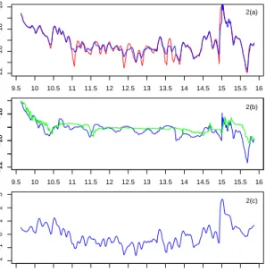
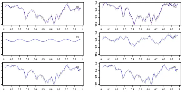
In Chapter 6, we examine the performance of our estimators in Monte-Carlo simu-lations and discuss implications for application. We present some simulation results for our pre-averaging type estimators for a situation with simplified but practical model pa-rameters. From the empirical analysis, we have observed the following on the volatility curve and microstructure noise of ultra-high-frequency data: (i) the typical U-shape over a trading day is mainly the feature of the intensity; (ii) the tick-time volatility estimator is in general smoother than the clock-time volatility and intensity estimators; (iii) the effect of microstructure noise on spot volatility estimation is very small. Moreover, issues con-cerning the quality of pre-averaging method are also discussed. The overall conclusion is

that the pre-averaging estimator is robust to the different types of noise considered here; however, it performs poorly for small sample sizes due to its slow rate of convergence.

Conclusions are discussed in Chapter 7. Appendices (A), (B) and (C) correspond to the proofs of Chapters 3, 4 and 5, respectively. Throughout this dissertation the following notations are used: f(n) is the n-th derivative of a functionf;IA is the indicator function

ofA; and an integer part of a real number xis denoted bybxc. If not otherwise stated, all equalities and inequalities of random expressions are expressed in an almost sure sense.

Preliminaries

2.1

Brownian Semimartingales and Some Properties

In the last decades financial mathematics has grown very fast, and a lot of models for asset returns have been introduced, both in the discrete- and continuous-time settings. Among many continuous-time models, a standard model for log-price processes is a Brownian semimartingale, which is the solution of the equation

dX_t∗=µ∗_tdt+σ_t∗dWt fort∈[0, T], (2.1)

where µ∗_t and σ_t∗ are adapted c`adl`ag stochastic processes and Wt is a standard Brownian

motion. This model is a special case of the more general process called a semimartingale, which is defined as the sum of a local martingale and an adapted process with finite varia-tion on the compact interval1. For more details see Jacod and Shiryaev [49] and Protter [62], among many others. The semimartingale has been shown to be an appropriate choice for modeling arbitrage-free asset price returns; see e.g. Delbaen and Schachermayer [27]. The special model (2.1) is attractive and tractable for studying the behavior of price movement of financial products due to its simplified form and the various mathematical tools available for analyzing it. The most important component lying in the Brownian motion part, the volatility σ_t∗2, is mainly used in finance and econometrics for risk managing, option pric-ing, etc., since it explains the uncertainty in the price movement; see an early application of stochastic volatility in option pricing in Hull and White [45]. The process µ∗_t is the drift coefficient, which plays a less important role in the risk analysis, especially when one considers prices over a small period of time, such as a day or a shorter period.

In the high-frequency framework2 it is well-known that the integrated volatility over a given fixed time period [0, T] can be consistently estimated by the realized volatility (also

1

It can also be equivalently defined as a good integrator on a class of processes as introduced by Prot-ter [62].

2

meaning that the observationsXt∗1, X

∗

t2, ..., X

∗

tn over the fixed time interval [0, T] become more dense

asn→ ∞; it is therefore an infill asymptotic framework.

called realized variance, realized quadratic variation). That is n X i=1 X ∗ ti−X ∗ ti−1 2 P −→ Z T 0 σ_s∗2ds

as the number of subintervals n goes to infinity, where 0 = t0 < t1 < ... < tn = T

is a deterministic sampling (or a stochastic sampling under some stronger assumptions) with maxi|ti−ti−1| → 0 and T fixed. In fact the integrated volatility is the same as

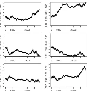
the quadratic variation of the model (2.1). Nowadays observing high-frequency data has become easier due to the efficiency of modern technologies. Figure 2.1 shows some examples of transaction data of assets traded on the NASDAQ stock exchange for April 1, 2014.

0 5000 10000 15000 20000 47.7 47.8 47.9 48.0 48.1 48.2 time pr ice 0 5000 10000 15000 20000 22.4 22.6 22.8 23.0 23.2 time pr ice 0 5000 10000 15000 20000 34.4 34.6 34.8 35.0 time pr ice 0 5000 10000 15000 20000 193.0 193.5 194.0 194.5 195.0 time pr ice 0 5000 10000 15000 20000 25.65 25.70 25.75 25.80 25.85 25.90 25.95 26.00 time pr ice 0 5000 10000 15000 20000 60.4 60.6 60.8 61.0 61.2 time pr ice 0 5000 10000 15000 20000 41.1 41.2 41.3 41.4 41.5 41.6 time pr ice 0 5000 10000 15000 20000 47.2 47.3 47.4 47.5 47.6 47.7 time pr ice

Figure 2.1: Some examples of high-frequency asset prices traded on NASDAQ for April 1, 2014. In the first row (from left to right): C, CSCO, INTC, and JPM and in the second row (from left to right): GM, IBM, MSFT, and VZ. X-axis is in 1-second resolution, i.e. 09:30 AM = 0 and 04:00 PM = 23400.

Asymptotic normality for the realized volatility has also been shown under a variety of assumptions. It is easiest to show in the case of deterministic equidistant observation times, that is when the price process is observed at every time point ti = (i·T)/n. We

obtain √ n ( _n X i=1 X ∗ ti−X ∗ ti−1 2 − Z T 0 σ∗_s2ds ) D −→ N 0, 2 Z T 0 σ∗_s4ds . (2.2) Therefore the resulting limit distribution is a normal variance mixture. To get a feasible version of this central limit theorem we can estimate the stochastic variance by the realized

power variation of order 4 called realized quarticity. This leads to Pn i=1 X ∗ ti−X ∗ ti−1 2 −RT 0 σ ∗2 s ds r 2 3 Pn i=1 X ∗ ti−X ∗ ti−1 4 D −→ N(0,1)

under some conditions on µ∗_t and σ∗_t. See Andersen et al. [3], [4], Barndorff-Nielsen and Shephard [7], [8], and the literature therein; the history about the application of the sum of squared increments in finance can also be found in these papers. Due to the popularity of this research area, a vast number of results for this model and its extension are devel-oped in the literature, including realized power variation, bipower or multipower variation, and cases of nonequidistant subdivision; see Barndorff-Nielsen and Shephard [8], [9], [10], and Barndorff-Nielsen et al. [13] among many others. In particular, the bi-/multipower variation has the benefit of testing for jumps in the price model. Furthermore, some of these results are generalized to provide functional limit statements; see the excellent work of Jacod and Shiryaev [49] and more recently Jacod and Protter [48]. We also recommend the more accessible work of Podolskij and Vetter [61] for understanding the main issues behind those deep theories and proofs. In particular, this work offers a clear explanation of stable convergence, which is a very useful tool for limit theorems of semimartingales observed at high-frequency. Of course we cannot mention all of the related results in this thesis; nevertheless, most of them can be found in the works of the authors mentioned and in the references therein.

2.2

Poisson Point Processes and Stochastic Intensity Models

A Poisson point process is a fundamentally useful process along with Brownian motion in the theory of continuous-time processes and is widely used for modeling arrivals or occurrences of events of interest. The main interest in this process is in its rate of arrivals, called intensity, which describes the average number of arrivals per unit of time. In many situations it is often useful to consider a Poisson process with a varying (or time-dependent) intensity called a nonhomogeneous Poisson process (NHPP). Such a process still has independent increments, but its stationary property does not hold anymore. Formally, given a probability space (Ω,F,P), let {Nt}t≥0 be a NHPP with respect to the natural

filtration

FN

t t≥0 with a deterministic non-negative real-valued intensity functionλt, i.e.

i) N0 = 0 a.s.,

ii) Nt−Ns is independent of FsN for all 0≤s≤t, and

iii) P(Nt−Ns =k) = exp n −Rt sλldl o ·( Rt sλldl) k k! fork∈N, 0≤s≤t, where FN

t = σ(Ns:s≤t) contains all information of the process up to time t. It turns

out that all realizations ofNt are right-continuous with left limits (c`adl`ag) which plays a

and Tankov [23]. Note that there are other equivalent definitions for Poisson processes which can be found in the literature. The representation used here is more convenient for our purposes. In particular, the associated arrival timesti := inf{t:Nt≥i} are stopping

times with respect to the natural filtrationFN

t t≥0 since{tn≤t}={Nt≥n} ∈ F

N t .

A more general process is the doubly stochastic Poisson process (or conditional Poisson process or Cox process), which allows for stochastic intensity; however, the intensity process is still independent of the Poisson process. More precisely, we first draw a realization of the random intensityλt, and once the whole path of λt is selected we generate a Poisson

process with this intensity. Having such a stochastic intensity is already interesting in practice, but we can go further and extend it to a more general point process with stochastic intensity that need not be Poisson anymore. This can be done by extending Watanabe’s characterization of the doubly stochastic Poisson process to a large class of stochastic intensity models—so large that it contains almost all point processes of practical interest; see Br´emaud [16, chapter II]. It has been pointed out that there is a connection between this point process and martingale dynamics (it is very helpful since many tools in martingale theory can be applied now). To easily see this relation we look at the compensated Poisson process with a constant intensityλ >0. It implies thatNt−λtis a martingale with respect

toFN

t ifNtis integrable.

The following definition of general stochastic intensity models is the one taken by Br´emaud [16]. In fact it is an extension of Watanabe’s characterization of doubly stochastic Poisson processes. Throughout this section we will always assume that a filtered probability space (Ω,F,{Ft}_t≥0,P) is given such that{Ft}t≥0 is right-continuous, i.e. ∩>0Ft+=Ft,

andF0 contains all P−null sets.

2.1 Definition (Br´emaud [16], Definition D7, p.27) Suppose that a point process Nt is

adapted to a filtrationF_t, and a non-negative F_t-progressive processλt is given such that

Z t

0

λsds <∞ P−a.s., for all t≥0,

holds. ThenNtis said to admit the Ft-intensityλt if the following condition holds:

E Z ∞ 0 cs dNs = E Z ∞ 0 csλs ds , (2.3)

for all non-negativeF_t-predictable processes ct.

In most applications the intensity is restricted to predictable, in which case the intensity process is uniquely determined. Indeed, a predictable version of the intensity is always available; see Br´emaud [16, Chapter II.4.]. The concept of predictable processes is very important in stochastic integral theory; for our present work it is enough to know that any left-continuous adapted process with right-hand limits (c´agl´ag) is predictable.

There are some essential remarks and results relating to our work when we look at stochastic intensity dynamics, and therefore we summarize them here for the purpose of refering to them later (all the proofs can be found in Br´emaud [16]). A review of the whole martingale theory with respect to Poisson point processes can also be looked up in, for example, Kuo [54] and Jacod and Protter [48]. See also a short review in Aalen [1].

2.2 Remark i) A doubly stochastic Poisson process is a special case of Definition 2.1

in that its intensity λt is restricted to being F0-measurable. Hence, conditionally

on F0, all information about the form of intensity is accessible. In formal language,

conditionally onF₀,Nt is anFt-NHPP.

ii) By setting the function cs = 1(0,τ](s) in (2.3) where τ is an Ft-stopping time3, we

have E[Nτ] = E Z ∞ 0 1_(0,τ](s)dNs = E Z ∞ 0 1_(0,τ](s)λsds = E Z τ 0 λsds . In particular, fort≥0 E[Nt] = E Z t 0 λsds ,

which also implies thatN0= 0 a.s.

iii) The corresponding arrival times ti := inf{t:Nt≥i} are Ft-stopping times.

More-over, for anyFt-adapted processφt,φti isFti-measurable or evenFt−_i -measurable if

φt is (left-)continuous. The stopping filtration at a random time τ is defined by

F_τ =σ{A∈ F : A∩ {τ ≤t} ∈ F_t, for all t≥0};

intuitively, it contains all information up to the random timeτ. The strict pastFτ−

is defined by

F_τ−=σ(A∩ {t < τ}, A∈ Ft, t≥0).

ParticularlyFτ−⊂ Fτ. See Br´emaud [16, Appendix A2].

iv) The following important properties are listed in Theorem T8, Br´emaud [16, p.27]:

a) Nt is non-explosive, i.e.Nt<∞ P-a.s. fort≥0.

b) Mt:=Nt−

Rt

0λsds is anFt-local martingale.

c) If yt is an Ft-predictable process such that E

h Rt 0|ys|λsds i < ∞ for all t ≥ 0, thenRt 0ysdMs is anFt-martingale. 3_{Sinceτ is anF}

t-stopping time, we have that{τ≤s} ∈ Fsfor alls, and therefore{τ≥s} ∈ Fs+=Fs

by the right-continuity of the filtration. Thusct= 1(0,τ](t) isFt-predictable (Ft-adapted and left-continuous

v) According to b), for a sequence of Ft-stopping times τn ↑ ∞, Nt∧τn− Rt∧τn 0 λsds is an F_t-martingale. Therefore E h Nt∧τn−Ns∧τn Fs i = E Z t∧τn s∧τn λudu Fs .

Letting τn go to infinity, we obtain

E h Nt−Ns Fs i = E Z t s λldl Fs

ifλtis assumed to be bounded. This yields that independent increments do not exist

in this general setting. Moreover, ifλt is continuous, and therefore predictable, then

lim t→s 1 t−sE h Nt−Ns Fs i =λs P−a.s.,

which reminds us of the classical definition of intensity functions.

vi) The boundedness of λt (which we shall always assume in our work) implies that

E[Nt] < ∞ and Mt is a square integrable Ft-martingale. Therefore we can avoid

working with local martingales. Moreover, by Doob-Meyer’s decomposition theorem

the compensator ofM2

t, denoted by< M >t, is equal to

Rt

0λsds. This result is useful

as we can now apply many properties of stochastic integration with martingales

as integrators such as Itˆo’s isometry or Burkholder-Davis-Gundy’s inequalities, see

e.g. Kuo [54, Theorem 6.5.8] and Jacod and Protter [48, p.39] respectively.

2.3

Nonparametric Curve Estimation: Spot Volatility

Esti-mator

In this section we will discuss statistical methods used to derive the main parameter in the asset price model (2.1). First it is interesting to have a brief look at some (nonparametric) techniques that are mainly used for estimating underlying curves, particularly in nonlinear regression and density estimation. We begin by thinking of a scatter plot of some data which could have a very complex structure. Our aim is to fit an appropriate curve to it. In nonlinear regression there are two approaches: the first one is the parametric approach, in which we fit a linear (which is normally biased) or a polynomial regression function to the scatter plot. To do this we would need to deal with the choice of the polynomial degree, say

p. It is clear that largepcan reduce the modeling bias but it can also cause high variability as the number of parameters is too high. In order to avoid the problem of specifying a model, the second approach of nonparametric fitting may be used. A lot of methods are developed in the nonparametric estimation literature, and some of them apply locally on the data set. The most common tools are kernel type estimators, local linear/polynomial fittings, wavelet thresholdings, and spline smoothings. All of these methods have their own advantages over the others, which can be seen in detail in many textbooks; we recommend H¨ardle and Linton [42] and chapter 2 of Fan and Gijbels [30] for an overview of these

smoothing techniques in the density estimation and regression analysis contexts. Local polynomial fitting in particular is intensively discussed in the latter. Instead of reviewing nonparametric devices in the connection with those topics, we prefer to discuss some of the techniques mentioned above in the volatility curve estimation context.

As mentioned in the beginning of this chapter, the integrated volatility can be con-sistently measured by the sum of squared increments observed with high-frequency. To extract the time-varying spot volatilityσ∗_t2, the most intuitive way is to proceed as though the volatility process were constant on a small neighborhood. Then we can filter the re-alized volatility to get an approximation of the spot volatility at a specific time point

to∈[0, T], i.e. given high-frequency observations Xt∗1, ...X

∗ tn of the model (2.1) 1 2h X to−h<ti≤to+h X ∗ ti−X ∗ ti−1 2 ≈ σ∗2(to)

for a small window h > 0. By assigning smaller weights for data points that are remote from the interested time point to, a lower modeling bias will be obtained. This procedure

leads to the kernel-based estimator introduced by Kristensen [53] and Fan and Wang [33], i.e. b σ_t∗_o2 := n X i=1 1 hK ti−to h X ∗ ti −X ∗ ti−1 2 , (2.4)

where K is a kernel function satisfying regularity conditions, and h is the bandwidth depending on n (recall that the high-frequency framework (or infill asymptotics) is being applied, i.e. we assume that more and more observations on the fixed interval [0, T] are available asngoes to infinity). Since this quantity only estimates the volatility at a single time pointto, the whole volatility line is therefore obtained by applying this local estimator

to a grid of points. Having spot volatility estimates is convenient since we are now able to estimate any functional of the spot volatility such as the former integrated volatility, derivatives of spot volatility (needed in the case of differentiable processes), etc. In order to draw some asymptotic inferences, of course, we need to know more about the structure of this volatility curve. It is natural to assume that the volatility curve satisfies some smoothness condition since we still want to stay in the nonparametric context rather than specifying a parametric model for the volatility. The following asymptotic results are given under assumptions (A.1)−(A.4) and (K.1) in Kristensen [53].

2.3 Theorem (Kritensen [53], Theorem 3) Suppose that we have equidistant observations,

i.e.ti =iT /n. Then for any a→0with a/h→0 we obtain

sup t∈[a,T−a] _bσ_t∗2−σ_t∗2 = O_p(hα) + O_p log(n)/ √ nh ,

and if the bandwidth conditions nh → ∞ and nh2α+1 → 0 hold, we get the following

asymptotic normality: √ nhσ_b∗_to2−σ_t∗_o2 −D→ N 0 ,2σ∗_to4 Z R K2(x)dx , (2.5)

forto ∈(0, T), where α is the H¨older exponent of the volatility curve.

The same result is also obtained by Fan and Wang [33, Theorem 1] with a slightly different set of conditions on the volatility process and the bandwidth. They have shown that common volatility models in the literature (such as geometric OU process, Nelson GARCH diffusion process, CIR process) satisfy all these conditions.

As a matter of fact, the main concern in kernel-based methods is the choice of the smoothing window h, since it plays a crucial role in the complexity of the estimation. If the bandwidth is chosen to be small, then the bias will be small. However, the variance will increase since we have fewer data points in each small neighborhood. On the other hand, if the bandwidth is large then the variance will decrease, but we will get a larger bias term. Thus it is necessary to trade-off between these two terms in order to get the most appropriate choice for the smoothing window. Solutions to the bandwidth selection problem have been discussed for a long time, e.g. plug-in and cross-validation methods. The Plug-in method is more restrictive, as we might need to know a priori the smoothness of the curve. A more complicated data-driven bandwidth selection is therefore desirable in many situations, especially when the smoothness/roughness of the curve of interest is unknown; see e.g. cross-validation criterions in Silverman [68] and H¨ardle [40] for imple-mentations. Kernel estimation has also been applied to extract the stochastic intensity of point processes; see e.g. Ramlau-Hansen [63].

Apart from the bandwidth selection problem, kernel-type estimators have a weakness at their domain boundaries. Since kernel functions are normally chosen to be symmetric functions, the estimators will cause biases at the edges of their domain due to the lack of data points. To overcome this problem one can use one-sided kernel functions or reflection methods; see Zhang and Karunamuni [71] and Fan et al. [31]. A more efficient solution that is automatically adapted to boundaries is a local linear fit. This method basically fits a linear model to the scatter plot locally around the time point of interest (in contrast to the kernel-based method which fits only a constant to the local area). For a more detailed discussion about how it can reduce the modeling biases at the edges, we refer the reader to Fan and Gijbels [30]. To overcome boundary effects of spot volatility estimation (2.4) a local linear fit has been briefly discussed in Kristensen [53, section 4] by solving the following problem: min b0,b1 n X i=1 K ti−to h ˜ σ∗_ti2− {b0+b1(ti−to)} 2 ,

where ˜σ_t∗_i2 is an approximation of the spot volatility at time ti, leading to the local linear

estimate ofσ_t2_o∗ (to∈[0, T]) n X i=1 1 hK ∗ c ti−to h X_t∗_i−X_t∗_i−1 2 +o(1) , (2.6)

whereK_c∗ is the so-called equivalent kernel function; see Kristensen [53, eq. (9)] and Fan and Gijbels [30, chapter 3].

Instead of local linear fits, we can also apply higher-order polynomial fitting, which fits the scatter plot better and also reduce the modeling bias. However we will need to deal with the higher order of the polynomial. Another advantage of using local polynomial fitting is the ability to estimate higher-order derivatives of parameter curves, which is useful in, for example, the plug-in method (where the second derivative of the curve normally plays a role in the bandwidth size). In constrast to the parametric approach of polynomial regression, where the degree of polynomials is normally large, local polynomial fitting works locally. We will therefore generally require fewer parameters (controlled by the degree of the polynomial). Typically the degree p is m+ 1, where m is the smoothness order of the parameter curve; see Fan and Gijbels [30]. As can be seen in the literature, standard volatility processes are normally driven by a Wiener process, which has non-differentiable paths, so a local polynomial of degreep= 1 (local linear) should work well for the derivation of spot voaltility curves. For a detailed discussion of local polynomial fitting techniques, see Fanet al. [29] and Fan and Gijbels [30].

Other nonparametric methods such as Fourier/wavelet transforms and spline smoothing are also popular and can be applied to estimate spot volatility curves. None of these techniques will be applied or discussed further in this work, so we have omitted the detail and refer the reader to Malliavin and Mancino [55] and Mancino and Sanfelici [56] for a comprehensive treatment of Fourier transforms and to Fan and Wang [32] and Schmidt-Hieber [67] for wavelet thresholdings. We note that wavelet-based methods have shown to be nearly minimax (in rate) for a large class of functions when the smoothness level is unknown.

2.4

Microstructure Noise Models

It has been observed in practice that the naive volatility estimators discussed above are not consistent when the data is observed with high frequency, such as every minute or at a finer resolution; see e.g. Bandi and Russell [6]. This means that the model formation for arbitrage-free price processes is disturbed by some factors in the real asset market. The reason of this incompatibility lies in the so-called market microstructure noise, possibly induced by discreteness of prices, bid-ask spreads or price formation, etc. It produces a noisy component in the arbitrage-free price process (2.1), leading to non-robustness of standard volatility estimators when the sampling interval is too small. Therefore many practitioners prefer to investigate data over longer time intervals in order to obtain unbiased results. Using a coarser grid of data, gathered at, say, a 5-minute or 20-minute resolution, makes the naive estimators more robust. For example, given tick-by-tick data of a liquid asset observed over a trading day Y_t∗₁, ..., Y_t∗_n, one would measure the integrated volatility by

X

Y_τ∗_i−Y_τ∗_i−12, withτi =ti·K forK∈N, (2.7)

where the sum is taken over 0 < τi ≤ T with, e.g. K = 300 (if the trades are assumed

to be exercised nearly every second, 5-minute interval is equal to 300). This approach is quite popular in the early empirical finance literature. However, using such coarse data in

order to avoid microstructure effects is unacceptable from a statistical point of view, since it is unsatisfactory to throw away data, especially such a huge amount of information (for example, if prices are observed at every second and we use data at a 5-minute resolution, then in every 5-minute period we will ignore 299 data points in the analysis); see Zhanget al.[70]. As a result, many statistical methods dealing with microstructure noise have been discussed to fully exploit the information hidden in the high-frequency data.

Statistically we can view market microstructure noise as an observation error. For the analysis, observable log-price processes are normally assumed to follow an additive noise model

Y_t∗_i = X_t∗_i+εi fori= 1, ..., n, (2.8)

whereεi is assumed to be a noise with

E[εi] = 0 and Var[εi] = ω2<∞;

the latent log-price process X_t∗ satisfies the model (2.1) (no other assumption on the dis-tribution of noise is made). Independence between the noise ε and the price process X∗

is typically assumed for simplicity of the proofs, but it is not essential. For this overview we will consider only time-equidistant data ti = iT /n for i = 1, ..., n in order to avoid

complications.

To clarify why the standard realized volatility based on high-frequency observationsY_t∗_i

is an inappropriate quantity for the integrated volatility, we look at

E " _n X i=1 Y_t∗_i −Y_t∗_i−1 2 # =E " _n X i=1 X_t∗_i−X_t∗_i−1 2 # + E " _n X i=1 (εi−εi−1)2 # = Z T 0 σ_t∗2dt + 2nω2.

This expectation explodes as n goes to infinity (we assume that σ_t∗ is at least locally bounded), so that the variablility of the noise term dominates the variability of the latent process. Nevertheless, the standard realized volatility can be used to measure the variance of the microstruture noiseω2; see Zhang et al. [70].

To overcome this non-robustness problem, many methods dealing with microstructure noise have been introduced. Starting with the first idea of Zhou [72], the effect of the contamination is now counteracted by adding a bias correction term into the common realized volatility, leading to an unbiased estimate

n X i=1 Y_t∗_i −Y_t∗_i−1 2 −2 n X i=1 Y_t∗_i−Y_t∗_i−1 Y_t∗_i−1 −Y_t∗_i−2 .

Unfortunately, this estimate remains inconsistent since the variability is still too high; see also Zumbach et al. [73] for the comparison of this estimate with other methods in

simulation studies and applications to real foreign exchange data. The intuitive idea of using higher-lag covariance terms is proposed by Barndorff-Nielsen et al. [11].

Now we will demonstrate three main approaches that have been extensively used in the analysis of microstructure noise models in practice. The first approach is from the excellent work of Zhanget al. [70], which uses different time scales to construct a consistent estimator for integrated volatility. Their combination of sparse and frequent sampling, which is satisfying from an empirical as well as a statistical point of view, is given by

1 K K X k=1      X τ_i(k)∈Gk Y∗ τ_i(k)−Y ∗ τ_i(₋k)₁ 2      −n¯ n n X i=1 Y_t∗_i −Y_t∗_i−12, (2.9)

where the original set of grid points{t1, ..., tn}is now partitioned into K subgridsGk, k=

1, ..., K. Usually Gk is chosen to be n τ₁(k), τ₂(k), ..., τn(kk) o :={tk, tk+K, tk+2K, ...tk+nkK}and ¯ n = PK

k=1nk/K. The first term is the average over multiple grids of sparsely observed

realized volatility (compare with (2.7)), which reduces the bias and variance of the con-ventional volatility estimator. The second term is a slight modification of the realized volatility, which deals with the rest of the bias induced by the disturbanceε. As discussed in their work, the best result of the combination of these two different time scales can be attained by choosing the parameter K optimally with respect to mean squared error minimization. In particular the asymptotic properties when K → ∞ as n → ∞ for this estimator and related quantities, such as asymptotic variance estimator and the estimator of the noise spread, are provided in their work. The rate of convergence of ordern−1/6 is derived for this integrated volatility estimator. Furthermore, many ideas of how to con-struct robust estimators are fruitfully discussed in their work, both from statistical and practical standpoints.

Unfortunately, Zhanget al.’s estimator cannot, as one would expect, reach the optimal convergence rate ofn−1/4 from the parametric maximum likelihood estimator in Gloter and Jacod [36]. Zhang [69] has therefore improved their two-timescale estimator to a multi-timescale estimator which achieves the optimal rate. In fact, this estimator is a direct extension of the best estimator given by Zhang et al. [70], combining different, say H, timescales to build a rate-optimal estimator for the integrated volatility.

Using the idea of autocovariances, the second approach is the realized kernel approach proposed by Barndorff-Nielsenet al. [11] and has the form:

γ0(Y∗) + H X h=1 K h−1 H {γh(Y∗) +γ−h(Y∗)}, (2.10) where γh(Y∗) := n X j=1 (Y_t∗_i −Y_t∗_i−1)(Y_t∗_i−h−Y_t∗_i−h−1)

is the realized autocovariance with lag h of the price seriesY∗;K(x) is a weight function defined on [0,1] with K(1) = 0 and the flat-top property K(0) = 1 (the flap-top kernel is in fact needed to eliminate the bias caused by the additional noise). This estimate consists of the standard realized volatility (the first term) and the flat-top kernel smoothing terms (the second term); see Barndorff-Nielsen et al. [11]. If H = 0 the inconsistent volatility estimate, realized volatility, is recovered; if H = 1, it is equivalent to Zhou’s estimator, which is unbiased but still inconsistent. Thereby one can reduce the variability of the estimation induced by the noise factor by using many lags of autocovariances. In this way one can construct a consistent estimator that achieves the optimal rate of convergence as found in the multi-timescale setting. This approach is applicable to data with endogenous time points, such as transaction data, which make it more useful in real data analysis. It is noteworthy that the extension of the realized kernel with finite lags to the realized kernel with infinite lags can achieve the efficiency bound given in the parametric version of this problem; see Barndorff-Nielsenet al.[11, section 4.5]. However, this idea is of limited relevance in practice as we will not observe a sufficient number of returns to construct virtually infinite lags. For implementation and extensive empirical analyses of this method, we refer to Barndorff-Nielsenet al.[12]; in particular, the effect of market microstructure noise on real stock prices is demonstrated via realized kernels.

The last technique we demonstrate here is introduced by Podolskij and Vetter [60] and later on extended by Jacod et al. [47]. This approach relies on the natural idea of using realized volatility based on local averages ¯Y_t∗₀,Y¯_t∗₁, ..., where ¯Y_t∗_i is defined as the average of, say, H data points Y_t∗_i, ..., Y_t∗_i+H−1. By doing this the variance of microstructure noise in the pre-averaged terms can be reduced by a factor of 1/H. Lastly the bias induced by the added noise is taken care of by a bias-correcting term. This pre-averaging estimator is explicitly given by b C_Tn := 1 H 1 R1 0 g(u)2du n−H X j=0 4Y∗_tj2− 1 2H R1 0 g (1)_(u)2_du R1 0 g(u)2du n X i=1 Y_t∗_i−Y_t∗_i−12 (2.11) where 4Y∗_tj = H−1 X h=0 g h H Y_t∗_j+h−Y_t∗_j+h−1

is the average of the price increments weighted by a function g over the block of size

H; g is defined on [0,1]. This approach has some features which cannot be seen in the multi-timescale and realized kernel approaches: (i) it enables straightforward construction of consistent estimators for other power variations of the process X∗; in particular the asymptotic variance of the estimator (2.11) can be quantified by such a technique in order to get feasible central limit theorems; (ii) together with the concept of bipower (or multipower) realized volatility, it can be used to detect jumps in the price model and to construct jump-robust estimators; see Podolskij and Vetter [60]. Although the pre-averaging estimate can achieve the optimal rate of convergencen−1/4, its asymptotic variance is less efficient than that of the realized kernel. In fact, the realized kernel is shown to have the smallest asymptotic variance among these three approaches. We state the asymptotic normality of

the pre-averaging estimator below for the sake of referring to it later, as our method will be based on this technique.

2.4 Theorem (Jacod et al. [47], Theorem 3.1) Suppose that assumptions (H) and (K)

in [47] hold. Let the weighting functiongdefined on[0,1]satisfy: gis piecewise continuously

differentiable with piecewise Lipschitz derivativesg(1)_{,g(0) =g(1) = 0and}R1

0 g(u)2du >0. WithH =θ·n1/2+o(n1/4) we get n1/4 b C_Tn− Z T 0 σ∗_t2dt → Z T 0 γt dBt, (2.12)

with the asymptotic variance

γ_t2 = 4 R1 0 g(u)2du 2 · " Z 1 0 Z 1 ν g(u)g(u−ν)du 2 dν·θσ∗_t4 + 2 Z 1 0 Z 1 ν g(1)(u)g(1)(u−ν)du Z 1 ν g(u)g(u−ν)du dν·σ ∗2 t ω2 θ + Z 1 0 Z 1 ν g(1)(u)g(1)(u−ν)du 2 dν·ω 4 θ3 # ,

where the above convergence is in the stably-in-law sense (for more details see e.g.

Podol-skij and Vetter [61]), and B is another standard Brownian motion, being independent of

the original space where σ_t∗ lives. Moreover, the asymptotic variance can be consistently

estimated by Γn_T given in their work [47, eq.(3.7)] which leads to a feasible version of

the central limit theorem n1/4nCb_Tn−

RT 0 σ ∗2_(t)dto_/p Γn T D −→ N(0,1) as a result of stable convergences.

Of course we have not stated all conditions for which the asymptotic properties of these three estimators hold. We emphasize that what they all have in common is that their smoothing parameterH plays a crucial role in the estimation. Some solutions of how to selectHin practice are therefore discussed in these and related works. Apart from these three main approaches there are many approaches dealing with market microstructure noise in the literature. Recently, the method given by Bibinger and Reiß [15] and Reiß [64] has gotten more attention, as the asymptotic efficiency of parametric volatility estimation can be achieved. We still rely on the pre-averaging procedure because of the advantages mentioned earlier.

In empirical analysis it has been shown that the noise conditions given in model (2.8) are somewhat too restrictive, since the noise sequence exhibits correlation with/dependence on the efficient price process; see Hansen and Lunde [39] and Kalnina and Linton [52]. Nevertheless, all these methods are able to deal with noise structures more general than i.i.d. noise (however, it is much more complicated; see details in their works). The literature investigates not only the effect of additive noise on the realized volatility, but also noise

with more complex structures such as rounding noise, additive noise plus a rounding effect, or nonlinear market microstructure noise; see e.g. Delattre and Jacod [26], Rosenbaum [66] and Dahlhaus and Neddermeyer [25].

As one might notice, none of the estimators (2.9), (2.10), and (2.11) are necessary non-negative, which contradicts the positivity of the spot volatility. Nevertheless, this is likely to be irrelevant in the empirical analysis of high-frequency data, as it has been shown that the noise is sufficiently small such that these three main estimators give satisfactory results; see also our simulation in Chapter 6. Positive estimators for asymptotic variance based on the subsampling method have been proposed by, e.g. Kalnina [51].

Finally, it is noteworthy that all of these noise-robust estimators work quite well even in the noiseless model, i.e.Y_t∗_i =X_t∗_i for alli= 1, ..., n. As a matter of fact, the variability of the estimates is too high compared with the variability of the standard realized volatility due to the slower rate of convergence, n−1/4 versus n−1/2. Thus, there is no gain in using such estimates in the absence of noise; in other words, it is better to use standard realized volatility when one knows without doubt that the underlying price process is not contaminated or that the noise is almost negligible.

Time Change Model and Volatility

Decomposition

Instead of the classical semimartingale (2.1) which is normally considered in the usual timescale, called calender time or clock time, we want to look at asset price returns relying on a different time clock. This time clock is controlled by a stochastic process that reflects market activities. In this work our main interest is the investigation of the spot volatility (also called instantaneous volatility) of a time-changed price-model based on trading times. This model is a pure jump process which can be interpreted as an asset price model having price changes at every transaction time. The main contributions of this work are the introduction and theoretical investigation of a new volatility estimator based on the volatility decomposition obtained in this time change model. In this chapter we introduce our model, show the volatility decomposition, and discuss the implications for applications.

3.1

Time Change Model

The study of statistical and empirical relationships between stochastic time clock and price processes, particularly the link between market activities, price fluctuations, and asset returns, has been extensively discussed in the financial literature. There is convincing evidence of a correlation between price volatility and the number/volume of trades. The investigation began when the distribution of asset returns over a short time period, such as a day or shorter, was reported to be non-normal1. To recover the normality of price distribution many stochastic time change models have been proposed,2 in particular, a time-changed Brownian motion

dXt=σ(t) dWT(t) fort∈[0, T], (3.1)

1_{We note that the non-normality of asset returns of the standard diffusion model (2.1) can be directly}

seen when the volatility process is non-deterministic, in which case price processes are mixed normal.

2_{We briefly define a time change as a (possibly) stochastic non-decreasing functionT : [0,∞)→[0,∞)}

withT(0) = 0 andT(t)→ ∞ast→ ∞. Thus for an arbitrary function/processf and a time changeT, we havefT(t)=f◦ T(t), where◦is the mapping composition.

whereW·is a Brownian motion,σ(t) is a stochastic process, andT(t) is a time change pro-cess carrying some market infomation which has an impact on asset prices. For instance, T(t) could represent the accumulated volume up to the timet or it could be the accumu-lated number of transactions up to time tas well. The former is suggested by Clark [22] from a theoretical and practical perspective that subordinating a Brownian motion by a directing process—in his work the volume of trades—can achieve the normality of the price distribution. This model is therefore applied to real cotton futures price data to show the normality. Since then the link between market activities—measured by the trading volume and the number of trades—and price fluctuation or volatility has been frequently discussed. An´e and Geman [5] conclude that the main reason of the volatility change is rather the number of trades than their size. In particular they recover the normality of asset returns through this stochastic time change in high-frequency data sampling; see more discussions on this topic in Joneset al. [50], Plerouet al. [59] and Gabaix et al. [34].

In the following, asset returns depend on market activities at each time period in the sense that price processes are controlled by a stochastic time clock given in (3.1). Thus prices evolve slowly if there is not much new information, and they evolve faster if there is a lot of news related to the asset—both company-related and general market news. Now σ2(t) represents the price variation per stochastic time clock (in contrast to σ∗_t2 in the standard diffusion model (2.1), which represents the price fluctuation in the usual timescale, called calendar-time or clock-time volatility). Having the representation (3.1) for asset returns means that identifying the processXt is the same as identifyingσ(t) and

T(t). The leverage effect of the volatility and the price process is now introduced in the correlation between the Brownian motion, the tick-time volatility, and the time change. SinceT(t) need not be continuous, the resulting processWT(t) is allowed to have jumps.

In this work the stochastic time change T_t = Nt is a point process representing the

accumulated number of trades up to timet. SinceNt is a counting process,WNt is a pure jump process. The use of this kind of process for modeling asset returns is also supported by the work of Gemanet al.[35] and many others in the time change model literature. Recently a time-changed Brownian motion has been employed to model credit risk, leading to a solution of the first passage problem for a class of processes related to financial modeling; see Hurd [46]. Indeed, modeling arbitrage-free asset price returns with such a model is reasonable since it has been shown that: (i) under a no-arbitrage assumption, asset prices are semimartingales (see Delbaen and Schachermeyer [27]); and (ii) any semimartingale can be transformed into a time-changed Brownian motion (Monroe [57]). Therefore having a class of time-changed Brownian motions is tractable because it is as large as a class of semimartingales. Particularly the standard Brownian semimartingale R₀tσ∗_sdWs can be

transformed intoBRt

0σ∗2ds whereB· is another Wiener process.

3

Other time change models have been extensively studied in recent years, in particular a time-changed L´evy process, which allows for a more complex structure in the price models

3_{In contrast to the usual definition of time-changed Brownian motion, we do not haveT}

tto be a stopping

time with respect toFt in order to defineWTt. In our frameworkNt is a stopping time with respect to the

in order to cope with some stylized effects emerging in the financial market; see Gemanet al.[35], Carret al. [19] and Carr and Wu [20]. For a statistical treatment of such a model see Belomestny [14] and the reference therein.

Our model:

As mentioned above, instead of classical semimartingales we use a time change model based on trading times, more precisely

Xt=

Z t

0

σs dWNs fort∈[0, T], (3.2) where the directing processNtis a point process with intensityλtreflecting the accumulated

number of transactions up to time t, σ2_t is called the volatility per transaction time (also called the volatility per tick or the tick-time volatility), and W(·) is a standard Brownian motion. The simplest case is the case in whichσtandλtare non-random and in whichW(·)

and N· are independent; in this case, Nt is a nonhomogeneous Poisson process (NHPP).

In a more general setting these processes are stochastic and depend on past realizations of Xt and Nt. The leverage effect between W(·) and N· is replaced by some martingale structure; in fact,W(·) need not be Gaussian (see below).

Clearly, this model is a pure jump model whose jumps occur at every arrival time or transaction time ti := inf{t : Nt≥i} for i= 1,2, ..., since the counting process Nt is a

pure jump process having jumps of size 1. The intensity λt serves as an arrival rate of

transactions per unit of time. We denote byNT the number of all transactions on the time

horizon [0, T]. In (3.2) the processσtrepresents the price fluctuation per unit of stochastic

time and not the volatility per calendar time (the usual timescale). Nevertheless, we can define volatility per calendar time for this model as a portion of price variation per unit of time, see (3.3) below. In particular, we will show that by looking at this kind of time change model, clock-time volatility appears to be a multiplication of two factors: tick-time volatility and intensity. This result corresponds to the observation that market activities are strongly related to uncertainty of asset prices. We do not consider a drift term in our analysis as we are interested in price oscillations over short time periods such as a day or shorter, and therefore the drift term has less impact on the analysis.

3.2

Volatility Decomposition

We mainly focus on the estimation of spot volatility for the financial transaction-time model (3.2), which is not the function σ2_t. Rather, σ2_t represents the price variation per transaction time, which is different from the meaning ofσ_clock2 (t) in the classical clock-time diffusion model (say dXt = σclock(t)dWt). We therefore start with a model-independent

definition for spot volatility and clarify below its relation to the tick-time volatilityσ_t2. Let us assume that there exists a filtered probability space (Ω,F,(Ft)t≥0,P), where (Ft)t≥0 is

up to and including timet. For an asset price model X(t) we define vola2_t := lim ∆t→0 E(X(t + ∆t)−X(t))2 Ft ∆t . (3.3)

It is remarkable that in the classical diffusion model vola2_t does not depend on the point process, and under the assumption that σclock(t) is a right-continuous process with

left-limits adapted toF_twe have vola2_t=σ_clock2 (t).4 Therefore, we useσclock(t) in this work as

a synonym for volat, i.e. we define

σ_clock2 (t) := vola2_t.

In the transaction-time model considered in this work, we prove below that σ2

clock(t) =

σ2_t ·λt. We first present the assumptions for this result. To understand our assumptions,

note that in (3.2) we do not use the whole process W(·) but only the increments Ui :=

W(Nti)−W(Nti−1), which we now assume to be a martingale difference sequence.

3.1 Assumption The Xti at observation times ti follow the model Xti =Xti−1 +σtiUi,

where the ti are the arrival times of a point process Nt. We assume that there exists a

filtered probability space(Ω,F,(Ft)t≥0,P), whereF0includes all null sets and the filtration

(F_t)t≥0 is right-continuous such that

i) Nt is a point process admitting an Ft-intensity λt (as in Definition 2.1; see also

Br´emaud [16, Definition D7]); in particularλtis an Ft-progressive process andNtis

adapted to Ft;

ii) σ2_t is a non-negativeF_t-predictable process; in particularσ2_t isF_t−-measurable;

iii) Ui is Fti-measurable for each iwith

E h Ui Fti− i = 0 and E h U_i2 Fti− i = 1.

(Remark that for asymptotic consideration we will need a condition on higher mo-ments of this sequences, see Chapter 4.)

This point processNt is quite general, as one can see in Section 2.2, since it allows for

the dynamics of both processes λt and Nt as they react to each other. Under all these

assumptions, a leverage effect between all processes—the tick-time volatility, the intensity, the point process and the innovationsUi—can be constructed to account for the correlation

between market information, volatility, and asset prices. Note that no other condition on

4_Since E h (Xt+δ−Xt)2 Ft i =_EhRt+δ t σ 2 clock(s)dWs Ft i =_EhRt+δ t σ 2 clock(s)ds Ft i

, the result fol-lows ifσ2

the distribution ofUi is required. The martingale difference structure ofUi is satisfied, for

example, for an i.i.d. sequence with mean zero and unit variance.

Examples for processes which fulfill these assumptions are given at the end of this section. The natural filtration which satisfies the above conditions is

Ft=σ({Ns:s≤t},{λs :s≤t},{σs:s≤t},{UNs :s≤t}).

3.2 Proposition Suppose Assumption 3.1 holds. If σt and λt are continuous processes

we have

σ2_clock(t) = σ_t2·λt. (3.4)

Proof. See Appendix A.

Therefore, in the transaction-time model the volatility can be decomposed into the product of two curves which can both be identified from the data. There exists an intuitive interpretation of this decomposition in that the formula reflects the change of time unit. The formula says that

“volatility per time unit is equal to volatility per transaction multiplied by the average number of transactions per time unit”.

This formula clearly explains the model for interaction between market activities and volatility of price, i.e. in a more active business day, reflected by a high activity rate, the volatility for the economy is high.

A highlight of the decomposition is the ability to estimate both curves σ_t2 and λt

separately by various estimates, sayσb

2_{(t) and}

b

λ(t). We use these estimates in two ways: i) to construct an alternative estimator ofσ_clock2 (t) via

˜

σ2_clock(t) := σ_b2(t)·bλ(t);

ii) to look at the two curves individually in order to gain more insight about the cause and structure of volatility.

A well-known result in econometrics is that standard volatility estimators are not ap-propriate in a noisy model when the data is observed with high frequency. To study the effect of so-called market microstructure noise, an additive noise model is introduced, i.e.

Yti =Xti+εi, fori= 1, ..., NT.

The contamination εi is, for example, an i.i.d. noise with E[εi] = 0 and Var[εi]<∞. For

more details about this model and robust volatility estimates we refer to the next chapter (and also to section 2.4).