Managing Large Data Sets Using Support Vector Machines

(1)

DigitalCommons@University of Nebraska - Lincoln

Computer Science and Engineering: Theses,

Dissertations, and Student Research Computer Science and Engineering, Department of

8-2010

Managing Large Data Sets Using Support Vector Machines

Ranjini Srinivas

University of Nebraska at Lincoln, [email protected]

Follow this and additional works at: https://digitalcommons.unl.edu/computerscidiss

Part of the Computer Engineering Commons, and the Computer Sciences Commons

Srinivas, Ranjini, "Managing Large Data Sets Using Support Vector Machines" (2010). Computer Science and Engineering: Theses, Dissertations, and Student Research. 7.

https://digitalcommons.unl.edu/computerscidiss/7

This Article is brought to you for free and open access by the Computer Science and Engineering, Department of at DigitalCommons@University of Nebraska - Lincoln. It has been accepted for inclusion in Computer Science and Engineering: Theses, Dissertations, and Student Research by an authorized administrator of

(2)

by

Ranjini Srinivas

A THESIS

Presented to the Faculty of

The Graduate College at the University of Nebraska In Partial Fulfilment of Requirements

For the Degree of Master of Science

Major: Computer Science

Under the Supervision of Professor David R. Swanson

Lincoln, Nebraska August, 2010

(3)

Ranjini Srinivas, M.S. University of Nebraska, 2010

Adviser: David R. Swanson

Hundreds of Terabytes of CMS (Compact Muon Solenoid) data are being accumulated for storage day by day at the University of Nebraska-Lincoln, which is one of the eight US CMS Tier-2 sites. Managing this data includes retaining useful CMS data sets and clearing storage space for newly arriving data by deleting less useful data sets. This is an important task that is currently being done manually and it requires a large amount of time. The overall objective of this study was to develop a methodology to help identify the data sets to be deleted when there is a requirement for storage space. CMS data is stored using HDFS (Hadoop Distributed File System). HDFS logs give information regarding file access operations. Hadoop MapReduce was used to feed information in these logs to Support Vector Machines (SVMs), a machine learning algorithm applicable to classification and regression which is used in this Thesis to develop a classifier. Time elapsed in data set classification by this method is dependent on the size of the input HDFS log file since the algorithmic complexities of Hadoop MapReduce algorithms here are O(n). The SVM methodology produces a list of data sets for deletion along with their respective sizes. This methodology was also compared with a heuristic called Retention Cost RC which was calculated

using size of the data set and the time since its last access to help decide how useful a data set is. Accuracies of both were compared by calculating the percentage of data sets predicted for deletion which were accessed at a later instance of time. Our methodology using SVMs proved to be more accurate than using the Retention Cost

(4)

(5)

DEDICATION

(6)

ACKNOWLEDGMENTS

I would like to thank my advisor and committee chair, Dr. David R. Swanson for his guidance and encouragement throughout the course of my Master’s program. Besides his expertise, I really appreciate his patience and thank him for his editorial advice which was essential for the completion of this thesis. I would also like to thank Dr. Lisong Xu and Dr. Byrav Ramamurthy for their advice and serving on my examining committee.

I thank the members of the Holland Computing Center for their time and research resources. I would like to thank all my friends in the Computer Science department for their support and encouragement throughout my stay at UNL.

Finally, I would like to thank my parents, who so enthusiastically supported and encouraged me to make it through my Master’s program.

(7)

List of Figures

1.1 Flowchart depicting how Large Data Sets are managed using Support Vec-tor Machines in this study. . . 3 2.1 CMS Computing Distributed Hierarchy. . . 15 2.2 In this figure, a hyperplane classifies two classes of training data which is

two dimensional. The two classes of data are represented by squares and circles. The bold line, which is separated from the closest training vectors by distance γ is the hyperplane. The classification of triangle, which is an unknown sample, is done by determining which side of the hyperplane it falls. In this example, the prediction for the unknown sample would be square. . . 18 2.3 In this figure, a hyperplane classifies two classes of training data which

is two dimensional by allowing error ξi in classification. The two classes

of data are represented by squares and circles. The bold line, which is separated from the closest training vectors by distance γ is the hyperplane. 20 2.4 The figure shows the mapping Φ(.) of attributes of the input space to the

feature space by a Kernel Function. . . 21 2.5 Map Function creates a new output list i.e (key, value) pairs from an input

(11)

2.6 Reduce Function processes the output from the Map Function. It sorts the (key, value) pairs and groups them by the key values [2]. Courtesy [1] 26 2.7 HDFS Architecture. Courtesy [1] . . . 28 2.8 Allocation of a virtual Hadoop cluster and running jobs on it. . . 31 3.1 The graph shows the pattern of file access requests received from some IPs. 39 3.2 Figure shows a script used for submitting Hadoop Streaming jobs using

SGE on Prairiefire. . . 43 3.3 ARFF file for the log data. . . 45 3.4 A basic ROC graph showing five discrete classifiers. A discrete classifier

is one that outputs only a class label. Each discrete classifier produces an (FP rate,TP rate) pair, which corresponds to a single point in ROC space. (courtesy [3]). . . 52 4.1 Accuracy rates of cross-validation test of all the nine SVM classifiers

trained on different data sets. . . 56 4.2 Accuracy rates of all the nine SVM classifiers tested against different test

data sets. . . 58 4.3 Accuracy rates of top two classifiers “A” and “B” tested against different

test data sets. . . 58 4.4 ROC of all the nine SVM classifiers. . . 60 4.5 This figure shows the performance of the MapReduce programs used in

this study and also shows that they are scalable . . . 61 4.6 Flowchart depicting how Large Data Sets are managed using Support

Vec-tor Machines in this study. . . 62 4.7 Contents of Input HDFS Log File. . . 64 4.8 Contents of Input Data set Dump. . . 64

(12)

4.9 Contents of Final Deletion Report. . . 65 4.10 Performance of different classifiers against test data J . . . 68

(13)

List of Tables

2.1 An extended taxonomy of some existing and proposed caching algorithms. 10

3.1 Percentage of files being accessed by a single IP. . . 39

3.2 The training sets used in this study. A, B and C belong to February 2009; D, E and F belong to March 2009; G, H and I belong to April 2009. . . . 40

3.3 Confusion Matrix . . . 49

4.1 Cross Validation Accuracy rates of the nine classifiers . . . 56

4.2 Accuracy rates of the top two classifiers against real data. . . 57

4.3 Confusion Matrix of Classifier A . . . 59

4.4 Performance Metrics calculated using Confusion Matrix as discussed in 3.3.2. . . 59

4.5 Retention Cost Metric calculated for some randomly picked data sets. . . 66

(14)

List of Algorithms

1 SVM Algorithm . . . 19

2 SVM Algorithm with a Kernel Function K() . . . 22

3 To create Delete-List - Mapper . . . 37

4 To create Save-List - Mapper . . . 37

5 To compute the number of times a file was accessed - Mapper . . . . 38

6 To compute the number of times a file was accessed - Reducer . . . . 38

7 To extract the IP from which a file was accessed - Mapper . . . 40

8 To extract the IP from which a file was accessed - Reducer . . . 40

9 To calculate the age of a file - Mapper . . . 41

10 To calculate the age of a file - Reducer . . . 41

(15)

Chapter 1

Introduction

This thesis proposes and demonstrates a methodology that could be used to solve management problems involving large data sets using Support Vector Machines. Ne-braska, being a US CMS Tier-2 site [4], stores terabytes of data and is a good candi-date for the “Big Data” problem. Disk space is required for new data sets constantly arriving from Fermilab and for older data sets frequently used by physicists for their analysis [4]. This manageability issue is addressed in this thesis. We present a policy which aides in cleaning up a specified amount of disk space intelligently and conve-niently in a very short time. All this data is being archived at FermiLab, Chicago and can be retrieved at a later point of time, if need be.

CMS Physics data consists of data sets in turn comprised of a number of files. Metadata maintained by the Dataset Bookkeeping Service (DBS) contains the map-ping between these files and the data sets they belong to. In order to identify the data sets to be deleted, we first identify the files that could be deleted. The more files belonging to a data set that are identified as less useful, the better are the chances of it to be considered for deletion. Currently, files and data sets are being deleted manually. This approach is very time consuming and is quite error prone. It is hard

(16)

to identify and consider many contributing factors which are important in making a decision whether a file or a data set needs to be deleted. Since the user community is big and consists of multiple researchers there exists competing interests with regard to retentivity of data sets. There is absence of a clear criteria. This makes it impera-tive to find a different methodology for cleaning the disk space other than just using the latest access time or random deletion. The methodology developed here studies the pattern of deletion which has occurred in the past. A machine learning algorithm is used to learn this pattern and helps classify the data sets by classifying the files belonging to these data sets. The tool which is presented here not only automates this process using this methodology but also is more accurate and objective in predicting a list of candidate data sets to be deleted.

Apache Hadoop is a powerful tool used in the analysis of Big Data [5]. Hadoop provides the power of scanning and analyzing terabytes of log data using a collection of commodity servers working in parallel. SVM is a Kernel based technique used for classifying files into those which need to be retained and those which could be deleted [6]. The MapReduce programming model is used in conjunction with SVM (Support Vector Machines) to arrive at a list of files or data sets to be deleted.

Nine different training sets (A to I), three from each month of February, March and April of the year 2009 were created from the HDFS logs. There was also a training set created by randomly sampling all these nine training sets. Classifiers were developed from each of these training sets. These classifiers were tested against test sets belonging to the same time frame and against test sets belonging to different time frames, since the objective was to choose the classifier that could be useful in classifying files which are created and accessed in the future months after the classifier was created. Their classification performance was analyzed using various statistics like accuracy rates and receiver operating characteristic graphs as discussed

(17)

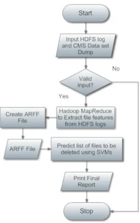
Figure 1.1: Flowchart depicting how Large Data Sets are managed using Support Vector Machines in this study.

in Chapter 4. The classifier with best classification performance was chosen. Weka, an open source machine learning suite developed at the University of Waikato in New Zealand was used in this study. It is a suite with an interface to various machine learning algorithms. For training a support vector classifier, it implements John Platt’s sequential minimal optimization (SMO) algorithm [7]. Figure 1.1 shows the way in which this classifier is used to classify data sets.

A heuristic, namely Retention Cost was also used to classify the data sets. Here, data sets were predicted for deletion based on their Retention Cost values and the pre-diction accuracy was compared to that of the SVM based methodology developed in this thesis. The SVM based methodology outperformed the Retention Cost heuristic

(18)

and thus could be used to solve similar problems involving large data sets.

The remainder of this thesis is organized as follows. Related work and back-grounds of Hadoop MapReduce Framework, Support Vector Machines and Weka, a Data Mining Software in Java have been discussed in Chapter 2. Chapter 3 explains data pre-processing and data collection methods, using SVMs for developing a clas-sifier, and performance analysis used in this study. It also discusses computation of Retention Cost heuristic. Results and discussions are given in Chapter 4. Finally, Chapter 5 concludes this thesis with overall discussion and future work.

(19)

Chapter 2

Background

2.1

Related Work

Various approaches to managing large data sets in different areas of research were studied. A method of functionally classifying genes by using gene expression data using SVMs to exploit prior knowledge of gene function to identify unknown genes of similar function from expression data was introduced in [8]. In [9] an SVM based method was used for predicting the propensity of a protein to be soluble or to form an inclusion body on overexpression in Escherichia coli. [10] proposed an SVM approach to stock trading in which an SVM classifier was successfully applied to forecast rela-tive performance within the oil sector. [11] proposed Combining Tag Cloud Learning with SVM classification to achieve Intelligent Search for Relevant Blog Articles. [12] explored the possibility of analyzing Massive Astrophysical Data sets using Hadoop. The applicability of MapReduce to spatial data processing workloads was studied in [13] where the excellent scalability of MapReduce was confirmed in that domain. [14] presents an efficient MapReduce algorithm for analyzing large collections of evo-lutionary trees this year in 2010. They conclude that MapReduce is a promising

(20)

paradigm for developing multi-core phylogenetic applications. Jeff Hammerbacher from Cloudera presented Analyzing petabytes of data with Hadoop at CERN Com-puting Colloquium in August, 2009 and claimed HDFS was storing over 700 TB of High Energy Physics (HEP) data. [15] concludes that MapReduce is a good choice for basic operations on large data sets for Machine Learning. In this study, we combine Hadoop MapReduce with SVMs to develop a methodology for managing large data sets.

We also discuss the literature on Hierarchial Storage Management, Caching Algo-rithms and Clustered File Systems in the following sub-sections in this chapter.

2.1.1

Hierarchical Storage Management

CMS Computing Distributed Hierarchy discussed in Section 2.2 is analogous to Hier-archical Storage Management (HSM). HSM supports backing up data to economical storage devices like magnetic tape drives and optical discs. Depending on the usage pattern, data is stored and migrated on different types of storage media. Storage media is categorized based on cost and speed of retrieval when access is required. The usage pattern is monitored to make a decision as to which data can safely be moved to slower devices and which data should stay on the fast devices. For example, when a file is being accessed very frequently it is stored on a high-speed storage de-vice like hard disk drive arrays, which is of high-cost. When the same file is accessed infrequently it is migrated to a slower but less expensive form of storage like mag-netic tape. It is transparent to the user when a file is being retrieved from backup storage media; this file is then moved back to a disk drive. HSM is thus a policy based management for archiving data by using storage devices economically. The first implementation of HSM was by IBM on their mainframe computers [16].

(21)

2.1.2

Caching Algorithms

The Retention Cost heuristic is in some sense a caching algorithm based on time and size criteria for deleting data sets. Caching algorithm aim to keep information that will be used in the future and to discard information that will not be used for the longest time in future. Some of the caching algorithms are discussed here.

• Least Frequently Used (LFU): In the Least Frequently Used (LFU) algorithm

the cache keeps the files which are really needed and discards the ones that aren’t needed for the longest period based on the access pattern. A counter is maintained to count how often a file is accessed i.e. the counter corresponding to a file gets incremented each time it is accessed. The file with least counter value is discarded first [17][18].

• Least Recently Used (LRU): The Least Recently Used algorithm removes the

file that was referenced the longest time ago with the underlying assumption that the files that have been used recently will need to be used again soon [18][19].

• Least Recently/Frequently Used (LRFU): [18] shows that there exists a

spec-trum of policies that subsumes the well-known LRU and LFU policies in the form of the LRFU. LRFU is formed by how much more weight we give to the recent history than to the older history.

• LFU with Dynamic Aging (LFUDA): LFUDA is a variant of LFU. It is based

on LFU-Aging policy that considers both the access frequency of a file and its age. A dynamic aging policy is used which adds the cache age factor to the reference count when a new object is added to the cache or when an existing object is referenced again. When a file is discarded its key value gets assigned

(22)

to the cache age instead of adjusting all key values in the cache. This ensures that the cache age is less than or equal to the minimum key value in the cache [20][21].

• Most Frequently Used (MFU): The MFU algorithm also known as

Fetch-and-Discard replacement algorithm, in contrast to LFU discards objects with highest frequency with the assumption that an object with a large frequency counter has had its fair share of diskspace and it’s time for some other object to get it’s turn. This algorithm is used to deal with the case such as sequential scanning access pattern, where most of recently accessed objects are not reused in the near future [22][23].

• Most Recently Used (MRU): In contrast to LRU, the MRU algorithm discards

the most recently used objects first. This caching mechanism is used when access is unpredictable and determining the least most recently used section of the cache system is a high time complexity operation [24][25].

• First In First Out (FIFO):: The FIFO algorithm has a list which contains the

file that arrived first at the front of the list and the rear of the list has the most recent arrival. This algorithm assumes that older files are not used often and when there is requirement for disk space it discards the file at the front of the list [26].

• Greedy-Dual-Size (GDS): The GDS algorithm considers the size and cost

infor-mation. It assigns a cost/size value to each object. Costs such as latency and network bandwidth can be explored although the cost is set to 1 in the simplest case. GDS assigns a key value to each object which is computed by summing the object reference count, the cost information divided by its size. Thus, recency

(23)

for an object is taken into account by inflating a key value (cost/size value) for an accessed object by the least value of currently cached objects [27][28].

• GDS with Frequency (GDFS): GDFS is a variant of the Greedy Dual-Size policy,

it also takes into account frequency of reference. This algorithm is optimized for more popular, smaller objects in order to maximize object hit rate. A key is assigned to each object computed as the object’s reference count divided by its size, plus the cache age factor [20].

• Lowest Relative Value (LRV): The LRV algorithm computes the lowest relative

value for each object using access time, frequency and size information. The object with the lowest relative value is discarded [29][30].

• Stor-serv: [31] proposes the concept of Quality of Service (QoS) ideas used in

networking to be applied to storage systems for giving differentiated services to users.

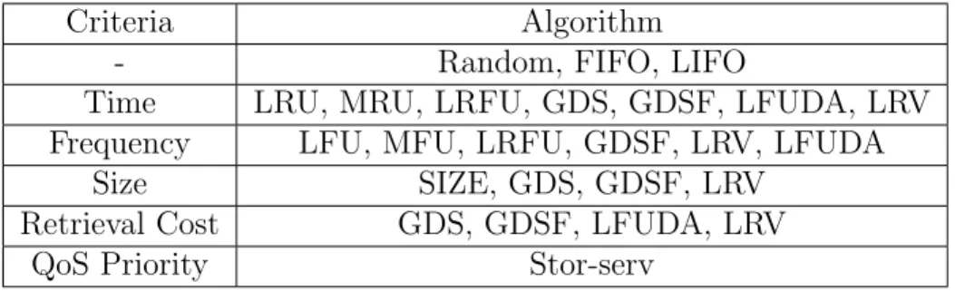
Table 2.1 lists some caching algorithms along with their criteria to make replacement decisions. Time, frequency and size are the most commonly used criteria. Algo-rithms like FIFO and LIFO do not require any such information to make replacement decisions. There are different possible criteria and the trend in cache replacement algorithms is towards finding functions that integrate most of it to a single value [32].

2.1.3

Clustered File Systems

Clustered File Systems are mounted simultaneously on multiple servers. The cluster is transparent and it appears as just a file system to the clients. We now discuss some

(24)

Table 2.1: An extended taxonomy of some existing and proposed caching algorithms.

Criteria Algorithm

- Random, FIFO, LIFO

Time LRU, MRU, LRFU, GDS, GDSF, LFUDA, LRV

Frequency LFU, MFU, LRFU, GDSF, LRV, LFUDA

Size SIZE, GDS, GDSF, LRV

Retrieval Cost GDS, GDSF, LFUDA, LRV

QoS Priority Stor-serv

of the clustered file systems which are closely related to the Hadoop Distributed File System (HDFS).

• Lustre: Lustre is a distributed file system with a “Shared Nothing”

architec-ture. Developed as a research project at Carnegie Mellon University it was later acquired by Sun Microsystems, which in turn was acquired by Oracle Corpora-tion. A Lustre file system consists of a metadata server (MDS) which contains a metadata target (MDT) per filesystem to store metadata such as filename, directories, permissions and file layout. Data is stored on object storage targets (OSTs) on object storage servers (OSSes). Clients are provided with read and write access through the standard POSIX interface [33].

• dCache: dCache is a disk-caching system jointly developed by DESY (Deutsches

Elektronen Synchrotron) and FNAL (Fermi National Accelerator Laboratory). It consists of an Admin node to run the administrative services and modules to manage pools of storage. There could be one or more pool nodes with pools. Door nodes provide I/O access through SRM or GridFTP to the stores. Door services are installed on the single Admin node. A pnfs node is used to map logical names to physical locations. By providing a single name space across the entire pool of disk servers it makes it look like a single, giant disk system to the users [34].

(25)

• IBM General Parallel File System (GPFS): The General Parallel File System

(GPFS) is a high-performance shared-disk clustered file system developed by IBM. Individual files are striped into blocks and stored across multiple disks. This provides higher input/output performance since the reading and writing of these blocks happens in parallel. Data loss is prevented by having multiple copies of each block written to the physical disks on the individual nodes using RAID controllers. The metadata including the directory tree is distributed and thus avoids single point failure [35]. It is also possible to have just two copies of all files and completely opt out of RAID-replicated blocks [36].

• Google File System (GFS): Google File System (GFS) is a distributed file system

where clusters are built from commodity hardware developed by Google Inc. A GFS cluster consists of a single master and multiple chunk servers and is accessed by multiple clients. Files are divided into chunks of fixed size. The master assigns each of these chunks with a unique chunk handle. Data loss is prevented by replicating chunks on multiple chunkservers. These chunkservers read and write data using the chunk handles. Metadata of the file system which includes the namespace, access control information, the mapping from files to chunks, and current locations of chunks is maintained by the master. Interaction between the client and the master consists only of metadata operations, all data operations happen at the chunkservers [37].

• Hadoop Distributed File System (HDFS): HDFS is highly influenced by GFS.

It is a framework written in Java which supports data-intensive distributed applications and is open source. It contains a master server known as the name node which maintains the filesystem namespace and the metadata of all the files and directories present in the filesystem tree. File access by the clients

(26)

are regulated by the name node. Files are striped into blocks of 64MB by default and these blocks are stored on worker nodes known as data nodes. For reliability, each block is replicated and stored on multiple data nodes. The data nodes receive instructions from the namenode for block creation, deletion and replication. They manage the storage attached to the nodes on which they run and are responsible for storing and retrieving blocks as requested by the clients and/or namenode. The name node has the information of how many HDFS blocks a file consists of and the data nodes on which these blocks are stored. File access by the clients are regulated by the name node [5]. HDFS is discussed more in detail in Section 2.4.3.

Clustered file systems are like IBM GPFS are available only on specific platforms on which the vendor has implemented them [38]. There are a lot of similarities between GPFS and HDFS and it is interesting to discuss their similarities and dis-similarities. Both GPFS and HDFS are designed to store very large quantities of data on datacenters built from commodity hardware. GPFS is commercial whereas HDFS is open source. Files are split into blocks and stored on different nodes under both these file systems. The block-size in HDFS is 64MB or more whereas the block-sizes in GPFS are under 1MB and thus are much smaller. Having many blocks of files fills up the filesystem’s indices very quickly. HDFS has lesser numbers of blocks due to larger block-size, this reduces the storage requirement of the Namenode. HDFS does not expect reliable disks, so instead stores copies of the blocks on different nodes. The failure of a node containing a single copy of a block is a minor issue, dealt with by re-replicating another copy of the set of valid blocks, to bring the replication count back up to the desired number. In contrast, while GPFS supports recovery from a lost node, it is a more serious event, one that may include a higher risk of data

(27)

be-ing (temporarily) lost. Namenode failure in HDFS becomes a sbe-ingle point of failure, but in GPFS single point of failure is avoided by having distributed metadata. In HDFS the MapReduce programming paradigm is supported and the location of data is made known to MapReduce programs for them to run near the data. Massively parallel programs are written in the MapReduce style. GPFS makes location of the data transparent since the applications do not need this information.

2.1.4

Prominent Users of Hadoop

There are many organizations and applications that use Hadoop extensively. Here is an incomplete list of prominent users of Hadoop [39]:

1. Yahoo: The Yahoo Search Webmap is a Hadoop application that runs on a more than 10,000 core Linux cluster and produces data that is now used in every Yahoo! Web search query. There are multiple Hadoop clusters at Yahoo, each occupying a single datacenter or fraction thereof. No HDFS filesystems or MapReduce jobs are split across multiple datacenters; instead each datacenter has a separate filesystem and workload. Yahoo has the largest installation of Hadoop.

2. Facebook: Facebook has the second largest installation of Hadoop. Hadoop is used to store copies of internal log and dimension data sources and is used as a source for reporting, analytics and machine learning.

3. Amazon Web Services: They provide a web service called Amazon Elastic MapReduce which hosts Hadoop framework running on the web-scale infras-tructure of Amazon Elastic Compute Cloud (Amazon EC2) and Amazon Simple Storage Service (Amazon S3) for their customers to perform data-intensive tasks

(28)

for applications such as web indexing, data mining, log file analysis, machine learning, financial analysis, scientific simulation and bioinformatics research. 4. Cloudera, Inc: Cloudera provides Hadoop professional training and support for

Hadoop. They also provide Cloudera’s Distribution for Hadoop to make it easy to set up, configure and use Hadoop [40].

5. Linkedin: Hadoop is used for discovering People You May Know and other fun facts [41].

6. Twitter: Twitter uses Hadoop for ad hoc analysis of data collected from its famous microblogging service, but the platform also crunches data for use by live tools on the site, including Twitter’s name-search function.

Areas of Applications of Hadoop: [40] discusses how Hadoop complements existing data management solutions with new analyses and processing tools. It provides a platform for consolidating data from various sources and delivers immediate value to a variety of vertical markets like:

1. Health and Life Sciences: Hadoop is used in drug discovery and development analysis. It also facilitates patient care quality and program analysis.

2. Telecommunications: Network performance and optimization is computed using Hadoop. Call Detail Record (CDR) analysis can also be done.

3. Financial Services: Risk analysis, fraud detection, security analytics, CRM, credit scoring and customer loyalty are also being determined using Hadoop. 4. Government: Hadoop can be used in determining energy consumption, carbon

footprint management, fraud detection and cybersecurity. It can also be used for compliance and regulatory analysis.

(29)

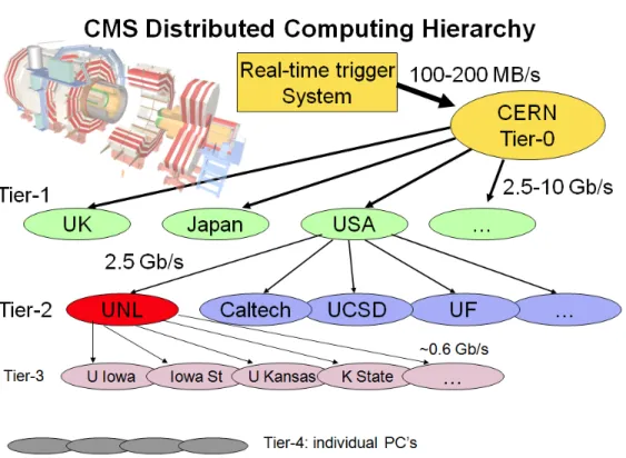
Figure 2.1: CMS Computing Distributed Hierarchy.

5. Web and Digital Media Services: Ad targeting, analysis, forecasting and opti-mization could be done using Hadoop.

2.2

HDFS logs used in this study

Nebraska is one of the eight US CMS (Compact Muon Solenoid) Tier-2 sites. CMS is a High-Energy Physics experiment, the results of which are being stored using Hadoop Distributed File System (HDFS) at the University of Nebraska-Lincoln. Fig-ure 2.1 shows the highly distributed computing system being used for processing and analyzing CMS data. The data goes through the following transformations before it reaches a physicist sitting in Nebraska. This holds for the other US CMS Tier-2 sites as well [4]:

(30)

• Raw data is processed at the Tier-0 center at CERN - the world’s largest particle

physics laboratory in Geneva, Switzerland. Firstly, raw data is transformed into reconstructed data.

• Reconstructed data is then transformed to analysis-oriented data (AOD).

Com-putational limitations at CERN make all the necessary transformations impos-sible at CERN and resort to seven Tier-1 centers worldwide for further trans-formations.

• Fermilab is the US Tier-1 center; it transforms the AOD data to

physicist-specific ntuples. Several copies of AOD data is maintained at Fermilab which undergoes processing every time improved calibrations and algorithms are able. All the available resources are used for this task and there are none avail-able for user analysis tasks, due to which the data is transferred to about thirty five CMS Tier-2 sites, Nebraska being one among eight in the US [42].

• The skimmed sub-samples of data from Fermilab reach Nebraska which provides

support for the analysis work of physicists and the required simulation capacity. Along with data transferred from Fermilab it houses user generated data and disk space is made available for temporary caching of samples being simulated by physicists.

Nebraska has made a cautious decision of choosing Hadoop for storing the CMS data. This thesis includes the development of a tool which analyzes gigabytes of Hadoop logs using MapReduce and SVM, is a product of investigation of how to manage data sets of very large scale.

(31)

2.3

File Classification Methods via Support

Vector Machines

Machine learning is concerned with the development of algorithms which enable the machine to learn and perform tasks. Support vector machines (SVMs) are a set of related supervised learning methods used for classification and regression [43]. SVM is a classifier derived from statistical learning theory by Vapnik and Chervonenkis [44]. It belongs to a family of generalized linear classifiers. It is a classification technique that seeks to find a hyperplane that partitions the data by their class labels and at the same time avoid over-fitting the data by maximizing the margin of the separating hyperplane. It makes a binary classification based on a separating hyperplane on a remapped instance space. Thus the goal of the classification is to remap the input vectors onto a multi-dimensional space so that the instances are linearly separable.

SVMs learn from labeled examples from a training set including both positive and negative samples. A hyperplane which classifies the positive and negative data in the training set is found based on the attributes of data in the training set. Many such hyperplanes which separate the data exist. The one that achieves maximum separation needs to be chosen and only one such hyperplane exists [45]. Such a hyper plane achieves good separation since it has the largest distance to the nearest training data points of any class [43].

The data points nearest to the margin on both sides are called support vectors. From the data and its labels the SVMs learn a mapping function. A kernel function, which is a dot product, is used in finding the hyperplane by remapping input feature vectors. Once the hyperplane is found, unlabeled examples from the test are classified based on the support vectors.

(32)

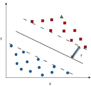
Figure 2.2: In this figure, a hyperplane classifies two classes of training data which is two dimensional. The two classes of data are represented by squares and circles. The bold line, which is separated from the closest training vectors by distance γ is the hyperplane. The classification of triangle, which is an unknown sample, is done by determining which side of the hyperplane it falls. In this example, the prediction for the unknown sample would be square.

Formalization: We represent each sequence by a feature vector which is nothing but a collection of the attributes in vector format. The goal is to correctly classify data in calculating the SVM. The decision boundary must classify all points correctly and should prevent data points from falling into the margin. Letn be the dimension of the feature vector and {x1, , xn} be the representation of a sequence x and let

yx{1,−1} be the class label ofx. The feature vectors of the training set are used to

build the classifier. Weight vector w is of the same dimension as the feature vector and it is represented as w = {w1, , wn}. The label of the sequence is predicted as

1 if wx+b ≥ 1 and it is predicted as -1 if wx+b ≤ 1 where, b is a threshold [4].

(33)

i) if yx= 1;wx+b≥1

ii) ifyx=−1;wx+b ≤1

The equation of the margin γx is given by

γx =yx(wx+b)

The value of γ determines the accuracy of SVMs in predicting the label of the se-quence. Ifγ is positive, it implies that the prediction is correct and a negative value of γ implies that the prediction is incorrect. The values of the weight vector w and threshold b are updated every time there has been an incorrect prediction. We now present a simple algorithm of an SVM [46]. In this algorithm, the weight vector w Algorithm 1SVM Algorithm

Require: w0 ⇐0, b0 ⇐0, k ⇐0

Require: R⇐ Radius of the vector most distant from the origin of vector space while mistakes are made on training setdo

for i = 1 to N do if yi(wk+b)≤0then wk+1 ⇐wk+ηyixi bk+1 ⇐bk+ηyiR2 end if end for end while

and the threshold b are initialized to 0. k keeps count of the number of incorrect predictions which is also initialized to 0. R is the radius of the hypersphere and is initialized to the maximum distance between the origin of the hypershere and a training vector. N is the total number of training vectors. η is the rate of learning. The decision hyperplane is given by the equation

(34)

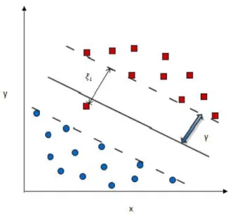
Figure 2.3: In this figure, a hyperplane classifies two classes of training data which is two dimensional by allowing error ξi in classification. The two classes of data are

represented by squares and circles. The bold line, which is separated from the closest training vectors by distance γ is the hyperplane.

The final weight vectorw is in the form [46]

w=

N

X

i=1

αiyixi (2.2)

where αi is the number of incorrect predictions made on the example. By using 2.1

and 2.2, the equation for the hyperplane becomes

h(x) = sgn

N

X

i=1

αiyihxi, xi+b) (2.3)

The representation of the data is in dot products.

Soft Margin Classifier [45]: In real world scenarios the decision boundaries might appear curved and there could be no straight line dividing the data points into two different classes in the data space. It is desirable to have a smooth decision boundary

(35)

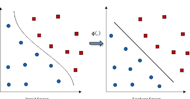
Figure 2.4: The figure shows the mapping Φ(.) of attributes of the input space to the feature space by a Kernel Function.

which ignores a few data points. By doing this, it is straight instead of being curved around some outliers. Thus, we allow error ξi in classification. ξi are just “slack

variables” in optimization theory [47]

           wxi+b ≥1−ξi yi = 1 wxi+b ≥ξi yi =−1 ξi ≥0 (2.4) We need to minimize 1 2||w|| 2₊_C n X i=1 ξi (2.5)

(36)

Kernel Trick: A separating hyper plane is used in the classification of linear data. However, in real world problems the data sets are mostly non-linear. In such cases, kernels are used to non-linearly map the input data to a high-dimensional space. The new mapping is then linearly separable [45]. The space xi are in is called the Input

space and the space of Φ(xi) after transformation is called Feature space. Linear

operation in the feature space is equivalent to non-linear operation in input space [47].

As discussed, we know that the data is represented in dot products. The dot product allows us to use kernels which implicitly remap and compute dot products. An SVM algorithm using kernel function K(x, y) for some vectors x and y is as below [46]. Thus, [47] Kernel trick allows SVM’s to form nonlinear boundaries. The Algorithm 2SVM Algorithm with a Kernel Function K()

while mistakes are made in for loop do for i = 1 to N do if yi(PN_j₌₁αiyjK(xj.x) +b)≤0then αi ⇐αi+ 1 b ⇐b+yiR2 end if end for end while

relationship between the kernel function K and the mapping

Φ(.)

is

K(x, x0) = hφ(x), φ(x0)i (2.6)

By specifyingK we indirectly specify Φ(.).K(x, x0) needs to satisfy the Mercer condi-tion in order for Φ(.) to exist. A real valued functionK(x, y) is said to fulfill Mercer’s

(37)

condition if for all square integrable functions g(x) one has [48]

Z Z

K(x, x0)g(x)g(x0)dxdx0 ≥0 (2.7)

Kernel Functions The idea of the kernel function is to enable operations to be performed in the input space rather than the potentially high dimensional feature space. Hence the inner product does not need to be evaluated in the feature space. We want the function to perform mapping of the attributes of the input space to the feature space. The kernel function plays a critical role in SVM and its performance. It is based upon reproducing Kernel Hilbert Spaces [49] [50].

K(x, x0) = hφ(x), φ(x0)i (2.8)

If K is a symmetric positive definite function, which satisfies Mercer’s Conditions,

K(x, x0) = ∞ X m amφm(x)φm(x0), am ≥0 Z Z K(x, x0)g(x)g(x0)dxdy ≥0, g∈L2 (2.9)

then the kernel represents a legitimate inner product in feature space. The training set is not linearly separable in an input space. The training set is linearly separable in the feature space. This is called the “Kernel trick” [49] [51].

The four types of Kernel Functions usually used with SVM are: 1. Linear Kernel K(x, x0) = (x.x0+ 1)

2. Polynomial Kernel K(x, x0) = (kx.y+c)p

3. Sigmoid Kernel K(x, x0) =tanh(kx.y+c) 4. Radial Basis Kernel K(x, x0) = e−γ||x−y||2

(38)

For this study, we employed a Linear Kernel.

2.4

Hadoop MapReduce for feature extraction

Apache Hadoop is a powerful tool used in the analysis of Big Data. It is a framework written in Java and supports distributed computing. Hadoop provides the power of scanning and analyzing terabytes of data using a collection of commodity servers working in parallel [5]. Hadoop MapReduce is a programming paradigm and software framework which is used for writing applications that rapidly process vast amounts of data in parallel on large clusters of compute nodes [52]. An application is broken down into small fragments of tasks and each of these tasks are executed or re-executed on any of the compute nodes of the cluster [53]. The Hadoop Distributed File Sys-tem (HDFS) discussed in Section 2.4.3 is used to store data on the compute nodes. Scheduling and monitoring tasks are handled by the framework. The framework also takes care of re-executing failed tasks. In this study, CMS Data is stored using Hadoop Distributed File and HDFS logs are processed using Hadoop MapReduce, discussed in Section 2.4.1.

2.4.1

Hadoop MapReduce

MapReduce is a programming model for data processing and is used to write programs that run in the Hadoop environment [2]. Large volumes of data are processed in parallel by dividing the work into a set of independent tasks [1]. Each process consists of two phases - the Map phase and the Reduce phase and is leveraged by functional programming constructs. Data in MapReduce cannot be subject to any changes and thus are immutable. This is so, since the communication occurs only by generating new output (key, value) pairs which are forwarded to the next phase of execution by

(39)

Figure 2.5: Map Function creates a new output list i.e (key, value) pairs from an input list. Courtesy [1]

the Hadoop framework. This approach improves the performance of the system by overcoming the communication overhead which occurs in keeping data on the nodes synchronized [2][1].

2.4.1.1 Map Function

Figure 2.5 shows the input list which consists of FileSplits obtained by splitting the input file. This splitting has no dependency on the internal logical structure of the input file. For each FileSplit a map task, called Mapper, is created [53]. The mapper transforms each element individually to an output data element in a parallel manner. The output from the Mapper is a list of (key, value) pairs. The number of Mappers determines the level of parallelism. In this study, the right level of parallelism was chosen individually for each job based on the size of data being processed and the number of cores that were requested to run the job using Hadoop on Demand (HOD) which is discussed in Section 2.4.4. Mostly, 101 Mappers and 11 Reducers were used, since this resulted in adequate performance.

(40)

MapRe-Figure 2.6: Reduce Function processes the output from the Map Function. It sorts the (key, value) pairs and groups them by the key values [2]. Courtesy [1]

duce framework. The number of partitions is equal to the number of reduce tasks for the job.

2.4.1.2 Reduce Function

A reduce task is called a Reducer. As discussed in the previous subsection, the Reducer takes the output of the Mapper which is then sorted by the framework as its input. It iterates through this list of (key, value) pairs and combines the values corresponding to a set of distinct keys. The way these values are combined is dependent on the objective of the job. The Reducer also emits a list of (key, value) pairs. Its output is nothing but a summary of the Mapper’s output [1].

2.4.2

Hadoop Streaming

Using Hadoop Streaming any language that can read standard input and write stan-dard output can be used to write a MapReduce program [54][2]. Mappers and

(41)

Re-ducers receive their input on stdin and emit output (key, value) pairs on stdout [1]. Communication between the Mappers and Reducers happens via these (key, value) pairs.

In streaming, the representation of input and output is textual. The input to the Mapper can be any text, HDFS logs in our case. Mapper processes this text and writes (key, value) pairs to the stdout. This is in turn taken as the input by a Reducer and emits (key, value) pairs to the stdout. Thus, output from streaming programs is written in the format:

key \t value \n

2.4.3

Hadoop Distributed File System: HDFS

The Hadoop Distributed File System is a distributed file system which supports redundant storage of large quantities of data across multiple disconnected disks and makes it appear as a single storage unit. Its design is based on the design of the Google File System (GFS) as described in [37]. It is designed for storing very large files that are gigabytes or terabytes in size with streaming data access patterns that run on clusters on commonly available hardware available from multiple vendors, generally known as commodity hardware. Each file is split into HDFS blocks of size 64MB by default and these blocks are stored on datanodes [2]. An HDFS cluster has a master-worker architecture [55][2] where a namenode is the master node and datanodes are worker nodes.

• Name node: It is a master server which maintains the filesystem namespace and

the metadata of all the files and directories present in the filesystem tree. The name node has the information of how many HDFS blocks a file consists of and

(42)

Figure 2.7: HDFS Architecture. Courtesy [1]

the data nodes on which these blocks are stored. File access by the clients are regulated by the name node.

• Data nodes: These are the worker nodes which receive instructions from the

namenode for block creation, deletion and replication. They manage the storage attached to the nodes on which they run and are responsible for storing and retrieving blocks as requested by the clients and/or namenode.

HDFS Commands: The basic structure of an HDFS command is: hadoop fs <cmd >

Some of the basic HDFS commands used are listed below [1]:

• -lspath: Lists the contents of the directory specified in the path

• -mv srcdest: Moves the file or directory within the HDFS from src to dest

(43)

• -rm path: Removes the file or empty directory specified in the path

• -rmr path: Removes the file or empty directory specified in thepath and recur-sively deletes child entries, if any

• -put localSrc dest: Copies the file or directory from the local file system ( local-Src) into the HDFS (dest)

• -get src localDest: Copies the file or directory from the HDFS (src) into the local file system (localDest)

• -cat filename: Displays the contents offilename

2.4.4

Hadoop On Demand (HOD)

HOD enables the use of Hadoop with batch schedulers to provision virtual Hadoop clusters on a large shared physical cluster of nodes [56][57]. Hadoop clusters are pro-visioned on demand and the scheduling is handled by resource managers like torque. A request can be made forN number of nodes to a resource manager and the resource manager then provisions them with a Hadoop cluster. Thus, a virtual hadoop cluster is setup quickly and used [57]. After completion of the task at hand, the resources are freed by the HOD and henceforth, these nodes are made available again. While using HOD, Hadoop is not required to be installed on the cluster. A Hadoop tar ball can be provided by the user which is then distributed by HOD to all the nodes which are required to form the virtual Hadoop cluster.

HOD has the following components [57]:

• HOD Client: The HOD client is a Unix command that users use to allocate

Hadoop MapReduce clusters. The command provides other options to list al-located clusters and deallocate them. The HOD client generates the

(44)

hadoop-site.xml in a user specified directory. The user can point to this configuration file while running Map/Reduce jobs on the allocated cluster.

• RingMaster: The RingMaster is a HOD process that is started on one node

per every allocated dynamic cluster. It is submitted as a ‘job’ to the resource manager by the HOD client. It controls which Hadoop daemons start on which nodes. It provides this information to other HOD processes, such as the HOD client, so users can also determine this information. The RingMaster is respon-sible for hosting and distributing the Hadoop tarball to all nodes in the cluster. It also automatically cleans up unused clusters.

• HodRing: The HodRing is a HOD process that runs on every allocated node

in the dynamic cluster. These processes are run by the RingMaster through the resource manager, using a facility of parallel execution. The HodRings are responsible for launching Hadoop commands on the nodes to bring up the Hadoop daemons. They get the command to launch from the RingMaster.

• HOD configuration file: An INI style configuration file where the users first

configure various options for the HOD system, including install locations of different software, resource manager parameters, log and temp file directories, parameters for their MapReduce jobs, etc.

• Submit Nodes: Nodes where the HOD Client is run, from where jobs are

sub-mitted to the resource manager system for allocating and running clusters.

• Compute Nodes: Nodes which get allocated by a resource manager, and on

which the Hadoop daemons are provisioned and started.

The sequence of operations in allocating a cluster and running jobs is pictorially represented in Figure 2.8:

(45)

Figure 2.8: Allocation of a virtual Hadoop cluster and running jobs on it.

1. Using the HOD client on the Submit node, the user specifies the required number of cluster nodes.

2. Using a Resource Manager interface, a Resource Manager job which is a HOD process called RingMaster is submitted to the central server of the Resource Manager.

3. Jobs are assigned by the resource manager central server to the resource man-ager slave daemons on the compute nodes. The RingMaster process is started on one of the nodes.

4. Using another Resource Manager interface, the RingMaster runs the second HOD Component, HODRing.

(46)

5. The HODRing gets Hadoop Commands by communicating with the RingMas-ter.

2.5

Python

Python is defined as an “object-oriented scripting language” [58]. It is an object oriented programming language which is often used for scripting purposes. The pro-gramming paradigm of Python resembles that of dynamic languages like Perl and Ruby [59].

Here, python is used for coding the mapper and reducer scripts that are run on the hadoop framework via hadoop streaming [2]. The most frequently used python module is “re”. It provides regular expressions matching operations similar to those found in Perl [60]. Processing the HDFS logs was treated as a text processing task. The data structure “Dictionaries” were extensively used. Dictionaries are nothing but “associative arrays”. The algorithms used to process these HDFS logs in order to extract the features required by the SVMs have been discussed in Section 3.1.3.

2.6

Weka: Machine Learning Software

Weka stands for Waikato Environment for Knowledge Analysis and was developed at the University of Waikato in New Zealand [7]. It is an open source machine learning suite written in Java which provides an interface to various machine learning algo-rithms. It supports pre-processing of data sets and helps in evaluating performances of learning algorithms [61]. Weka has a graphical user interface, called the Weka Explorer, and a command line interface is also available. Both the Weka Explorer as well as the command line interface were used in this study.

(47)

The tools provided by Weka for data pre-processing are known as “filters”. Dif-ferent filters are available for discretization, normalization, resampling, attribute se-lection, transforming and combining attributes. After the creation of ARFF files as described in section 3.1.6, they were loaded into Weka and were preprocessed us-ing these filters. ReplaceMissus-ingValues and Discretization filters were used. Data pre-processing is discussed in Section 3.1.2.

Training schemes that perform classification are used to classify the preprocessed data. Many classification schemes like decision trees, rule learners, naive Bayes, decision tables, locally weighted regression, SVMs, instance based learners, logistic regression, voted perceptrons and multi-layer perceptrons are supported by Weka. Weka’s Sequential Minimal Optimization (SMO) implementation of SVM is used in this study.

Graphical and text based results are generated by the explorer. The performance of an SVM classifier can be determined by the confusion matrix which is part of the text based result (Section 3.3.2). The threshold curve with False Positive rate along the x-axis and True Positive rate along the y-axis gives the Receiver Operating Characteristics (ROC) described in Section 3.3.3.

Nine models were built in the Explorer from nine different training sets. After identifying the best classification model among the nine classification models, the un-known data which needed to be classified was used against this model at the command line interface of Weka.

(48)

Chapter 3

Materials and Methods

3.1

Data Collection

The SVM learning algorithm used in this thesis was trained on several training sets. The classification performance was examined using the test sets. We now discuss the preparation of these training and testing sets.

3.1.1

Data Source

HDFS logs for ninety days starting February, 2009 to April, 2009 were considered. These logs have information with regard to file operations of every file belonging to the subset of USCMS data stored at Nebraska.

3.1.2

Data Pre-processing

HDFS logs might contain log information pertaining to a file being accessed many number of times within a small period of time which could be due to a faulty process trying to access a file or a set of files over and over again. The logs could also contain information about files which were only used for managing the storage and which

(49)

cannot be considered in solving our problem. Features of such files become outliers in this study and it is imperative for the data being used for learning by the SVMs to be clear of such outliers. This data also had to be transformed to a format suitable for SVMs, to improve the performance. Hence, preprocessing was required.

3.1.2.1 Data Cleaning

The Weka Explorer was used for data cleaning. Weka reports the minimum, maxi-mum, mean and standard deviation values for all the attributes in a data set. This information is used to eliminate the outliers. Weka also reports the percentage of missing values in a data set. Using the filter, ReplaceMissingValues, missing values were replaced by the mean value for that attribute.

3.1.2.2 Discretization

It has been shown by [62] that discretization can help improve significantly the clas-sification performance of learning clasclas-sification algorithms such as SVMs. Weka’s discretize filter helps in converting numeric attributes to nominal. Equal-width bin-ning worked well with our data set. In Equal-width binbin-ning, the range of possible values is divided intoN subranges of the same size [63][7].

binwidth= maximumvalue_N−minimumvalue

In this study, the value with approximately the best classification performance was the final choice for N which was mostly 60 for each of the nine training data sets.

3.1.3

Training Data

From the HDFS logs, the list of files which were deleted were used to obtain the positive data sets. Likewise, the list of files which were not deleted was used to obtain

(50)

negative data sets. The features of deleted and not deleted files were extracted using Hadoop MapReduce. The features which were extracted are as follows:

1. Number of times a file was accessed in one month time frame 2. IP from which a file was accessed

3. Lifetime of a file in the same one month time frame

We also considered the CMS data set to which a file belongs to by using the data set IDs. This information was retrieved from a database maintained by Carl Lundstedt, one of the grid administrators at the Holland Computing Center at the University of Nebraska-Lincoln.

Using Hadoop MapReduce for feature extraction: We start by making two lists of filenames. The first list contains the files which were deleted in the three month time frame. It is used to generate the positive data sets used in the training data. We call this list, the “Delete-List”. The second list, the “Save-List” consists of files which were retained and it is used to generate the negative data sets. The algorithms used to create the Delete-List and Save-list using the MapReduce paradigm [2] are presented in Algorithm 3 and Algorithm 4.

Once these lists are prepared from the HDFS logs, we have mappers and their corresponding reducers written in Python to be used with Hadoop Streaming. Each Mapper-Reducer pair is designed and developed to extract one of the three features listed above. We briefly discuss how each of these features was extracted:

1. Number of times a file was accessed in one month: The number a times a file is being accessed is one of the most important factors to be considered while trying to make a decision with regard to its retentivity. The HDFS logs are considered

(51)

Algorithm 3To create Delete-List - Mapper

Require: Array containing filenames of deleted files, DeleteArray[ ]←0 for every line in HDFS logs do

if cmd=delete in line then

if word in line is a filename AND not in DeleteArray[ ] then add word to DeleteArray[ ]

end if end if end for

for every filename in DeleteArray[ ]do print filename

end for

Algorithm 4To create Save-List - Mapper

Require: Array containing filenames of saved files, SaveArray[ ]←0

Require: Array containing filenames of deleted files, DeleteArray[ ] created using Algorithm 3

for every line in HDFS logs do

if word in line is a filename AND not in DeleteArray[ ] then if word not in SaveArray[ ] then

add word to SaveArray[ ] end if

end if end for

for every filename in SaveArray[ ]do print filename

end for

line-by-line. While generating the positive data sets, every line of the HDFS logs is searched to see if it contains access information for files featured in Delete-List. This is achieved by the Mapper, AccessMapper.py coded in Python. The AccessMappaer.py outputs “hf ilenamei, 1”even though the hf ilenamei might

occur multiple times in the log file. This output from the Mapper is then taken as input to the Reducer, AccessReducer.py which sums the occurrences of each filename to a final count. Thus, the number of times a file was accessed is computed from the logs. The same is repeated for the files in Save-List. The

(52)

algorithm used to extract the access information is as below:

Algorithm 5To compute the number of times a file was accessed - Mapper for every filename in Delete-List do

create a hash map with filename as the key and a counter as the value end for

extract the filename in the current line look up the hash map for this filename if filename is found in hash mapthen

increment the respective counter end if

end for

print every (key, value) pair of hash map

Algorithm 6To compute the number of times a file was accessed - Reducer Require: counter←0

for every line in mapper’s output do key ←<f ilename>inline

value←1inline

while value of the key changes do print key, counter

counter←0 end while

counter←counter+value end for

2. IP from which a file was accessed: It was observed that most of the access requests were coming from a distinct set of IPs. It was also observed that files belonging to different data sets were being accessed from the same set of IPs. Thus, it is interesting to consider the IP from which a file was being accessed. We now discuss the algorithm used to extract the IP from which the corresponding file was accessed from the HDFS logs. It was observed that most of the files were being accessed from a single IP, so, only one IP per file has been considered in this study. Table 3.1 shows these observations from a few samples of HDFS logs.

(53)

Figure 3.1: The graph shows the pattern of file access requests received from some IPs.

Table 3.1: Percentage of files being accessed by a single IP. Month/Year Total No. of

Files No. of Files Accessed by One IP No. of files accessed by more than one IP Percentage of files accessed by a single IP Feb 2009 6145 5874 271 95.59 Mar 2009 6580 6142 708 89.3 Apr 2009 5470 5186 284 94.81

3. Age of a file: The duration of existence of a file is also used as a factor here. We provide SVM with this data which is used to determine whether a file needs to be deleted or not. Out of a one month time frame we list the filenames and their corresponding age for both categories of files - those deleted and those which were not deleted. The algorithms used to get this data from the HDFS

(54)

Algorithm 7To extract the IP from which a file was accessed - Mapper for every filename in Delete-List do

create a hash map with filename as the key and a counter as the value end for

extract filename and IP in the current line look up the hash map for this filename if filename is found in hash mapthen

assign IP to this key end if

end for

print every (key, value) pair of hash map

Algorithm 8To extract the IP from which a file was accessed - Reducer for every line in mapper’s output do

key ←<f ilename>inline value←IP inline

while value of the key changes do print key, value

end while end for

Table 3.2: The training sets used in this study. A, B and C belong to February 2009; D, E and F belong to March 2009; G, H and I belong to April 2009.

Training Set ID Positive Instances Negative Instances Total No. of Instances

A 5164 4085 9249 B 4467 4438 8905 C 4467 4139 8606 D 5752 4959 10711 E 4838 5688 10526 F 4479 5677 10156 G 3800 7680 11480 H 4968 6728 11696 I 3696 6728 10424

logs is presented here.

The algorithmic complexity of all these algorithms is O(n) and it depends on the size of the input log file.

(55)

Algorithm 9To calculate the age of a file - Mapper for every filename in Delete-List do

FirstAccess: create a hash map with filename as the key to hold first access timestamp

LastAccess: create a hash map with filename as the key to hold first access timestamp

end for

extract filename and timestamp in the current line look up the hash map for this filename

if filename is found in hash mapthen if value for key is unset then

assign timestamp to this key in FirstAccess end if

if value for key is set then

assign timestamp to this key in LastAccess end if

end if end for

print every (key, value) pair of both hash maps

Algorithm 10To calculate the age of a file - Reducer Require: dif f ←0

Require: DateArray[ ]←0

for every line in mapper’s output do key ←<f ilename>inline

value←dateinline

if value of the key changes then

calculate the difference between first and last file access timestamps; consider just the date leaving out the seconds and microseconds from the timestamp, diff

remove all the elements in DateArray[ ] end if

print key, diff end for

(56)

3.1.4

Test Data

The test data was also prepared from the HDFS logs. All features of the files i.e. the number of times a file was accessed in one month, the IP from which the file was being accessed and the number of days of existences of the file within the one month period were extracted from these HDFS logs using the algorithms in Section 3.1.3. Thus, the test data contained both positive and negative instances. The performance of each classification algorithm was tested against these test data sets.

3.1.4.1 Testing against training data belonging to the same time frame Three test sets were generated one each for February, March and April of 2009. The February test set was tested against all the three classifiers that were prepared using the HDFS logs from the same month, February, 2009. This experiment was repeated for March and April of 2009 as well. Results are discussed in Chapter 4.

3.1.4.2 Testing against training data belonging to a different time frame Among the nine classifiers, two classifiers with the best Classification Accuracy Per-centage and Receiver Operating Characteristic (ROC) were short listed and these were tested against test data prepared using a different month’s log data.

Having different test data helps in identifying the best classifier as it helps in evaluating the performance of the classifier when tested against test data belonging to a different time frame. This is a very important factor since the model which is developed here is intended for practical use at the Holland Computing Center to address a maintenance issue - creating more space for storage by eliminating files which are of least value. In other words, the classifier which has been developed

(57)

Figure 3.2: Figure shows a script used for submitting Hadoop Streaming jobs using SGE on Prairiefire.

based on log data of 2009 should be useful in classifying files which are created and accessed in the future months after the classifier was created.

3.1.5

Running MapReduce using Hadoop On Demand

(HOD)

MapReduce programs written in Python were run with Hadoop Streaming using Hadoop On Demand. Sun Grid Engine (SGE), an open source batch-queuing system [64] was used to submit Hadoop Streaming jobs to Prairiefire - a 90-node Beowulf cluster [65]. Figure 3.2 is an example of an SGE script which was used to submit jobs to the queue. The sge script helps in requesting the required number of cores for the virtual hadoop cluster.

(58)

It also contains the Hadoop Streaming command. Hadoop streaming jar comes with the Hadoop distribution and it facilitates MapReduce jobs. The option -mapper is used to specify the mapper, a python script that needs to be distributed to the nodes which perform the map function. Likewise, the option -reducer is used to specify the reducer used by the nodes to perform the reduce function. Options -input and -output give the HDFS path of the input and output files respectively. -file option is used to package an auxiliary file required by the mapper.

3.1.6

Creating an ARFF file for WEKA

An ARFF, Attribute Relation File Format was developed by the Machine Learning Project at the Department of Computer Science of The University of Waikato for use with the WEKA machine learning software. It is an ASCII file which contains a list of instances sharing a set of attributes [66], which is a standard way of representing data sets whose instances are independent, unordered and there is no relationship among these instances [7]. ARFF file structure is described using Figure 3.3. The name of the relation appears at the beginning of the file. @relation declaration associates a name with the data set. Here, the name of the relation is “logdata” and it is represented as

@relation logdata

Following the name of the relation is a block defining the attributes such as ID, AccessNumber, Age and IP. @attribute declaration specifies the name and type of an attribute.

@attribute ID numerical @attribute AccessNumber numerical

(59)

Figure 3.3: ARFF file for the log data.

@attribute IP numerical @attribute delete? yes, no

All the attributes take numeric values and are followed by the keyword numeric. delete? is the class value which is predicted from the values of other attributes.

The attribute definitions are followed by @data declaration in a single line denot-ing the start of the data segment. Every line corresponds to an instance and each instance is represented by the values taken by its attributes. Missing values, if any, are represented by a single question mark.

(60)

ARFF files for our study were created from the outputs of MapReduce processes which were discussed in Section 3.1.6.

Algorithm 11To create ARFF file for the log data Require: create a file with .arff extension

write

“@relation logData” into ARFF the file write

“@attribute ID numeric @attribute accessno numeric @attribute IP numer