Recurrent Multitask-Learning for Irregular Clinical
Time Series Forecasting
by
Suraj Subramanian
Submitted to the Graduate Faculty of
the School of Computing & Information in partial fulfillment
of the requirements for the degree of
Master of Sciences
University of Pittsburgh
2020
UNIVERSITY OF PITTSBURGH
SCHOOL OF COMPUTING AND INFORMATION
This thesis was presented
by
Suraj Subramanian
It was defended on
April 3rd 2020
and approved by
Dr. Dmitriy Babichenko, School of Computing & Information
Dr. Stephen Hirtle, School of Computing & Information
Dr. David G. Binion, University of Pittsburgh Medical Center
Copyright c by Suraj Subramanian 2020
Recurrent Multitask-Learning for Irregular Clinical Time Series Forecasting Suraj Subramanian, M.S.
University of Pittsburgh, 2020
Inflammatory Bowel Disease (IBD) is a group of chronic gastrointestinal disorders that are difficult to treat. Having no known cure, treatment courses can be long-term and ex-pensive. IBD flare-ups can happen without warning and there exists no objective criteria to measure the disease’s activity. Recently, Recurrent Neural Networks (RNN) have emerged as a state-of-the-art method in clinical time series analysis; building on recent work that apply RNNs to temporal patient data, this thesis explores methodologies for processing temporal clinical data, the feasibility of a deep RNN classifier to forecast the future healthcare uti-lization, and techniques to curb overfitting while training on a small dataset. This work shows that multitask learning is helpful to train stable models, and deep networks can be engineered to process small noisy datasets in the clinical domain.
Table of Contents
1.0 Introduction . . . 1
2.0 Background . . . 2
2.1 Inflammatory Bowel Disease . . . 2
2.2 Clinical Decision Support . . . 2
2.2.1 Deep Learning in CDSS . . . 4
2.3 Electronic Health Record . . . 6
2.3.1 EHR Analytics . . . 6
2.4 Artificial Neural Networks . . . 7
2.4.1 Training . . . 9
2.5 Deep Neural Networks . . . 9
2.5.1 LSTM . . . 10
2.5.2 GRU . . . 11
2.6 Machine Learning in IBD Research . . . 11
3.0 Prior Work and Motivation . . . 13
4.0 Data Description . . . 14
4.1 Features . . . 14
4.1.1 Drug Prescriptions . . . 14
4.1.2 Clinical Lab Results . . . 15
4.1.3 Diagnostic Procedures . . . 15 4.1.4 Surgeries . . . 16 4.1.5 Clinician Encounters . . . 16 4.1.6 Disease Descriptors . . . 16 4.1.7 Charges . . . 17 4.2 Model Inputs . . . 17 4.2.1 Missingness Metadata . . . 17
5.0 Methods . . . 19
5.1 Cross Validation for Time Series . . . 19
5.1.1 Naive K-fold Split . . . 19
5.1.2 Chronological Holdout . . . 20
5.1.3 Chronological Split with Overlap . . . 20
5.2 Model . . . 21 5.2.1 Encoder . . . 21 5.2.2 Classifier . . . 22 5.2.2.1 Activation Functions . . . 22 5.2.3 Regularization . . . 23 5.2.4 Multitask Learning . . . 23 5.2.4.1 Charges . . . 24
5.2.4.2 Diagnostics, Labs, Surgeries . . . 25
5.2.4.3 Replicated Targets . . . 25 5.3 Experiments . . . 25 5.3.1 Time Horizons . . . 26 5.3.2 Multitask Loss . . . 26 5.3.3 Architectures . . . 26 5.3.4 Baseline . . . 27 5.3.5 Evaluation Metrics . . . 27 5.4 Results . . . 28 6.0 Conclusion . . . 30 6.1 Future Work . . . 31
Appendix A. Confusion Matrices . . . 32
Appendix B. Loss Trends During Training . . . 33
List of Tables
List of Figures
1 Trend of research interest in EHR and DL . . . 4
2 ANN Architecture . . . 8
3 LSTM Cell . . . 10
4 GRU Cell . . . 11
5 Histogram of annual charges . . . 24
6 Baseline Confusion Matrices . . . 32
7 GRUD Confusion Matrices . . . 32
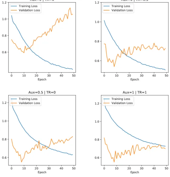
8 Training and Validation Loss Trend (50 epochs) - OL Data Split . . . 33
1.0 Introduction
Inflammatory Bowel Disease (IBD) is a group of chronic gastrointestinal disorders that are difficult to treat. IBD is a chronic disease requiring long-term care; managing the disease can be difficult owing to largely unpredictable responses to treatments. A characteristic of the disease is a sudden re-occurrence of symptoms even after an extended period of remission, known as flare-ups. Serious flare-ups may require complicated and intensive measures such as surgically removing a part of the colon. A possibility of knowing in advance which patients are likely to undergo such procedures can help care-providers design their treatment strategy. With the advent of electronic health records and machine learning, there is a surging interest to tackle these problems with predictive analytics. This thesis describes work done in this direction as part of a larger effort at the IBD Translational Research Center at UPMC. The primary aims of this work are to 1. Investigate the feasibility of using deep neural networks on a small clinical dataset, and 2. Explore if the irregular occurrence of medical events holds useful exploitable information. In this work, I apply techniques like multitask learning and parameterizing missing variables to help the model overcome data sparsity and approximate the distribution from lesser training examples. The results of this research indicate the usefulness of these techniques to stably train a complex model on a small dataset.
The rest of this thesis is structured as follows: Section 1 presents background information on IBD, Clinical Decision Support Systems (CDSS), Neural Networks and Deep Learning, EHR and EHR analytics, and current machine learning methods in IBD research. Section 2 talks about the prior work that this thesis builds upon. Section 3 contains a description of the variables used to train the model. Section 4 details cross validation schemes for time series, the architecture of the model, the experiment methodology, caveats and constraints regarding validation integrity, and the results. Section 5 consists of the conclusion and future recommendations in this line of research.
2.0 Background
2.1 Inflammatory Bowel Disease
Inflammatory Bowel Disease (IBD) is a class of chronic inflammatory disorders affecting the gastrointestinal tract. The specific causes of IBD are not known, and it is believed to result from genetic variations, environmental influences, alterations in gut flora and distur-bances in the immune system responses (Abraham & Cho, 2009), (Jostins et al., 2012). IBD and its major subgroups – Crohn’s Disease (CD) and Ulcerative Colitis (UC) – often ex-hibit patterns of remissions and flare-ups; response to treatments is largely unpredictable. A large number of IBD patients require hospitalization at some point in their lives, thus incur-ring heavy financial burden (Cohen, Larson, Roth, Becker, & Mummert, 2000), (Silverstein et al., 1999). Smaller groups of patients contribute disproportionately to overall expendi-tures (Click, Binion, & Anderson, 2017). Prognosticating the disease course among patients of IBD is difficult challenge because of varied responses to treatments. A standard strat-egy is systematic incrementalism – a slow-and-steady method of treatment as opposed to early intensive interventions like surgery. This can involve considerable trial-and-error before triaging onto the treatment plan that works for a patient. IBD greatly affects well-being and quality of life; two tools to measure disease severity are the Harvey-Bradshaw Index (Vermeire, Schreiber, Sandborn, Dubois, & Rutgeerts, 2010) and the SIBDQ (Han et al., 2000). One of their major shortcomings are they both are subjective measures and it is not easy to standardize these scores across a population. This study uses healthcare utilization charges as a proxy for how well or poorly a patient is doing.
2.2 Clinical Decision Support
The Office of the National Coordinator for Health Information Technology defines Clin-ical Decision Support Systems (CDSS) as what “provides clinicians, staff, patients, or other
individuals with knowledge and person-specific information, intelligently filtered or presented at appropriate times, to enhance health and health care” (Osheroff et al., 2007). The evolu-tion of CDSS has a trajectory similar to those of general decision support systems; classical CDS includes alerts, reminders, facilitation of computerized physician order entry (CPOE), and interactive dashboards analogous to many Business Intelligence (BI)/Analytics software. Initial systems in the 1960s were powered by Bayesian statistics and decision trees, with a pinch of early AI (Pople, Myers, & Miller, 1975). The underlying methods powering many of today’s CDSSs have come a long way from manually encoding clinician expertise and rules in knowledge bases. This is partly due to the proliferation of Electronic Health Record interoperability, and inexpensive computational means necessary to process Big Data.
Bright et al. report that CDSS have a favorable effect on prescribing treatments, fa-cilitating preventive care services, and ordering clinical studies across diverse venues and systems. In published research, there appears to be considerable evidence of CDSS efficacy in improving health care process measures, but sparse evidence with regards to predicting clinical outcomes (Bright et al., 2012). This can be attributed to a lack of significant evidence to the difficulty of evaluating CDSS in RCTs. A significant barrier to adoption of CDSS is vetting the reliability of the system’s recommendations. Probabilistic inference is often counterintuitive for humans and leads to physicians ignoring CDSS recommendations if they have made their decision (Bates, 1998). Many of the underlying ML models are “black-box” (i.e. lack interpretability). Experienced clinicians are likely to trust their judgements when at odds with a CDSS, and novice practitioners are likely not confident enough to make such an evaluation.
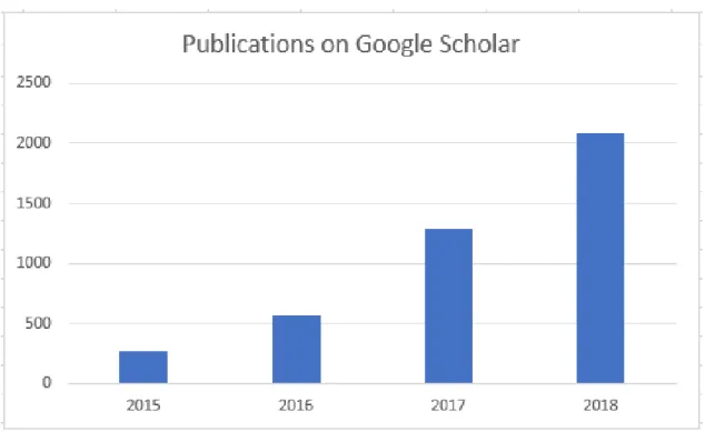
A majority of CDSS surveyed in Jaspers, Smeulers, Vermeulen, and Peute (2011) and Bright et al. (2012) haven’t moved beyond the basic features of classical decision support. As of 2009, only about 1.5% of 3000 surveyed hospitals report the use of “Comprehensive EHR” (Jha et al., 2009). On the other hand, in clinical informatics research there is a growing interest in using machine learning in a CDSS. A Google Scholar count of”electronic health record deep learning” evidences this (Fig. 1).
Figure 1: Trend of research interest in EHR and DL
2.2.1 Deep Learning in CDSS
A proliferation of electronic medical data has led to a rapid rise (Fig. 1) in the use of deep learning methods to analyze complex problems in healthcare. Some of the areas it has had major impact in are clinical imaging, genomics and EHR analysis.In an excellent survey of state-of-the-art applications of DL in healthcare, (Shickel, Tighe, Bihorac, & Rashidi, 2018) categorize current research in the field into 5 overarching tasks:
Information Extraction Parsing meaningful concepts from clinical notes, a difficult task for traditional ML compounded by the unstructured nature of this data.
Representation Learning Static hierarchical ontologies are often inadequate to capture complex interactions and subtle similarities often found among medical concepts. Repre-sentation Learning projects these concepts into high-dimensional vector space to encode natural relationships in an unsupervised manner.
out-come prediction - static, where the prediction is not constrained to temporal horizons (eg: single point identification of medical conditions), and temporal, where the model either relies on time-series data, or makes a prediction for a specific time window. Computational Phenotyping True to the spirit of ML, these studies allow the data to
speak for itself; unsupervised algorithms comb through large volumes of data to determine clusters of phenotypes indicative of an outcome of interest.
Clinical Text De-identification The use of RNNs to automatically deidentify Personal Health Information, to adhere to HIPAA guidelines.
Clinician notes are often unstructured, noisy and may contain non-standard medical jar-gon, which pose a challenge to vanilla ML and NLP methods, but are suitable for DL. (Liu, Ge, Mathews, Ji, & McGuinness, 2018) use word-embedding from CNNs to automatically expand abbreviations in clinical ICU notes. (Jagannatha & Yu, 2016) use LSTM and GRU to extract medical events from clinical notes. (Miotto, Li, Kidd, & Dudley, 2016) use de-noising autoencoders (an unsupervised DL algorithm) to build representations of the patient that encode latent patterns in their clinical events, and are predictive of diseases like dia-betes and schizophrenia. (Lasko, Denny, & Levy, 2013) use unsupervised DL methods for longitudinal clinical phenotype discovery from episodic EHR data. (Gulshan et al., 2016) use Convolutional Neural Networks (CNN) to detect diabetic retinopathy from ophthalmic imaging data with physician-like accuracy. (Lipton, Kale, Elkan, & Wetzel, 2015) trained a LSTM-RNN to recognize diagnoses from the patient’s full time-series data. (Choi, Bahadori, Schuetz, Stewart, & Sun, 2016) use a GRU-RNN trained on EHR to predict major clinical events in the future.
Despite their successes, deep learning approaches to health data suffer from important limitations, a prominent criticism is the lack of interpretability of the model’s predictions. In clinical settings a degree of interpretability is necessary, especially when being used to guide diagnoses and treatment decisions. Deep networks often require voluminous datasets; for less common disorders like IBD, it can often take several years to collect enough data to train a model. The quality of data directly influences the performance of a deep learning algorithm. Medical records are especially prone to noise, ambiguity, sparsity and heterogeneity, making it challenging to train a good model.
2.3 Electronic Health Record
An Electronic Health Record (EHR) system is a repository of electronically maintained information about an individual’s health status and care. An EHR represents the snapshot a patient’s state in time. While it can be thought of as a digitized version of a patient’s paper chart, the information collected can go beyond standard clinical data, offering a broader view of the patient. A comprehensive EHR contains information about billings and claims, patient demographics, medications, lab and test results, allergies, comorbidities and clinician notes. EHRs are built to share information among healthcare providers - so they contain information from all the clinicians involved in the patient’s care. At current rates of adoption, even a small hospital would have millions of records over a decade - an aggregate equivalent of centuries of doctor wisdom (Esteva et al., 2019).
2.3.1 EHR Analytics
Physicians often do not have the bandwidth to use every relevant prior medical record for their diagnoses. Given the volume of available data, statistical and machine learning models are better suited to uncover patterns in patient interactions and outcomes, predict the possibility of important events (eg: hospitalization, drug prescriptions, ER surgery), and estimate the efficacy of different treatment pathways.
A common use case for EHR Analytics is predictive risk assessment to improve patient outcomes or reduce costs. For example, the current incidence of early-onset sepsis (EOS) is 0.05-0.1% of all live births, but antibiotics are administered to 11% of infants born. Kaiser Permanente Northern California (an insurance company) used data mining and logistic re-gression to develop a risk-stratification model of EOS in infants. The model was trained on data points collected from the mothers’ and babies’ EHR (Escobar et al., 2013). The contin-uous aggregation of data in the EHR facilitates comparative effectiveness research identifying optimal interventions tailored to patient-level characteristics (Miriovsky, Shulman, & Aber-nethy, 2012). Large volumes of EHR data fed into a common data model has been used to predict the risk of heart failure, determine alternative medications and treatments, and
identify at-risk patients from patterns in healthcare utilization (Gotz, Stavropoulos, Sun, & Wang, 2012). Topic modelling and Natural Language Processing (NLP) analyses on inpatient psychiatric discharge notes have been used to predict psychiatric readmissions (Rumshisky et al., 2016). One group highlights the potential shortcomings of such approaches, namely the exclusion of disadvantaged populations and a myopic focus on short-term optimizations like cost instead of long-term health (Wharam & Weiner, 2012).
By its very nature, EHR data is challenging to analyze by automatic systems. EHR data is noisy, heterogeneous, and sparse. Non-standard reporting of lab results across different providers, missing values, and incorrect patient information can heavily skew the algorithm’s decision. Furthermore, its asynchronous nature is reflected in the irregular frequency of mea-surements among all features. A common approach to time-series dimensionality reduction is to represent all the values of a variable within a time window by its mean, described as Piecewise Aggregate Approximation (Lin, Keogh, Wei, & Lonardi, 2007). While this re-duces the complexity of the problem space, there are several pieces of information lost in this aggregation. Granular changes in values of lab or test results can be indicative of future outcomes. In aggregating, not only do these values regress to the average (which might lead to mispredictions) but any trends of change within the discrete time window is also lost. Concurrent variations in the patients’ attributes that might have phenotypic importance are diminished in aggregation.
2.4 Artificial Neural Networks
Artificial Neural Networks (ANN) are a class of Machine Learning (ML) algorithms that attempt to emulate the human brain in function. Over the past decades, ANNs have been at the heart of systems in myriad domains - financial analysis, petroleum exploration, missile guidance systems, and famously, early autonomous vehicles developed at Carnegie Mellon in the 1980s (Kim & Calise, 1997), (Ali, 1994), (Pomerleau, 1989).
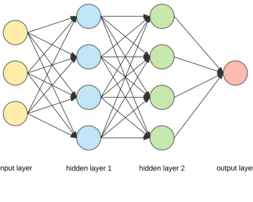
ANNs consist of artificial neurons - ‘cells’ that each accept weighted data points and output values based on the function encoded in each cell. One of the first artificial neurons
Figure 2: ANN Architecture
is the perceptron, a cell that takes several binary inputs to produce a single binary output. A simple example to demonstrate its use is in deciding whether to go to the beach. The output decision y can have a value of either 1 (go to the beach) or 0 (stay at home). To make this decision, the perceptron accepts inputs x1 (1 if the weather is sunny, 0 if it is
raining) and x2 (1 if you are alone, 0 if your friend accompanies you), and encodes their
relative importance in weights w1 and w2. The perceptron has a pre-defined function that
outputs a decision based on the inputs and weights. Suppose the weather is sunny but you have no company, and the decision function is given by
y=w1x1−w2x2
The ANN knows you love a sunny day more than anything; it has learntw1=0.9 andw2=0.3,
2.4.1 Training
An ANN typically has multiple layers of neurons (Fig. 2). The leftmost layer accepts input data; the rightmost layer outputs the decision. Between the two, there are a number of hidden layers where most of the data crunching takes place. Each neuron has a weight associated with it; they are initialized to a random value. Training an ANN involves feeding it input data, allowing the hidden layers to process the inputs to output a decision, and comparing it with the true (expected) decision. The difference in outcomes - “loss”- is then reduced by modifying the weights in each of the neuron layers until the network has attained a desired level of accuracy.
2.5 Deep Neural Networks
The advent of Big Data and faster computation has led to a newer paradigm in neural networks called Deep Learning (DL). Deep Neural Networks (DNN) work in a different fashion from ANNs. ANNs primarily learn a function that predicts the target from the input data with minimal error. DNNs first engineer new simpler features that are representative of the input, and then use these features to predict the target. This is achieved by tuning each neuron to have a very simple non-linear function. The DNN learns complex concepts by abstracting these simple representations. For example, it represents the concept of an image by combining simpler concepts like contours and shading, which are in turn composed of extremely simple representations like edges.
DNNs often have numerous hidden layers, which means more sequential operations on the data. This allows them to execute tasks which are too complex for traditional ML algorithms, such as detecting people and animals in images. Google Lens turns any smartphone camera into an oracle; pointing the camera to an object displays information about it (along with advertisements of where it can be purchased). Intelligent assistants like Alexa and Siri make use of DL to comprehend speech and respond appropriately. The sequential operations helps the model to retain “states” of information (similar to how humans process information
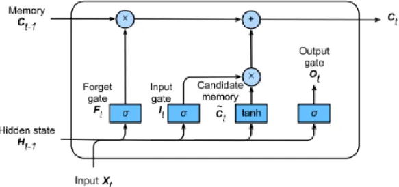
Figure 3: LSTM Cell
streams) and allows it to infer subtle differences and create representations of them.
Recurrent Neural Networks (RNN) are distinct from traditional feed-forward networks. In a feed-forward network, hidden layers send their outputs only in one direction. RNNs instead allow feedback within the hidden layers; the output of a neuron is not only sent to subsequent hidden layers, but it also forms part of the input to itself after a preset delay. There are two kinds of RNNs that are of interest in temporal EHR analysis - Long Short-Term Memory (LSTM) and Gated Recurrent Units (GRU).
2.5.1 LSTM
LSTM (Fig. 3) is a special type of RNN whose hidden state architecture attempts to emulate human information and memory processing (Gers, Schmidhuber, & Cummins, 1999). LSTM units have cell-states that maintain information over the entire sequence (“long-term memory”), and forget-gates that update the cell-state with every new piece of information the network processes. With sufficient training, the network learns which pieces of information are most important to the output, and “forgets” the others.
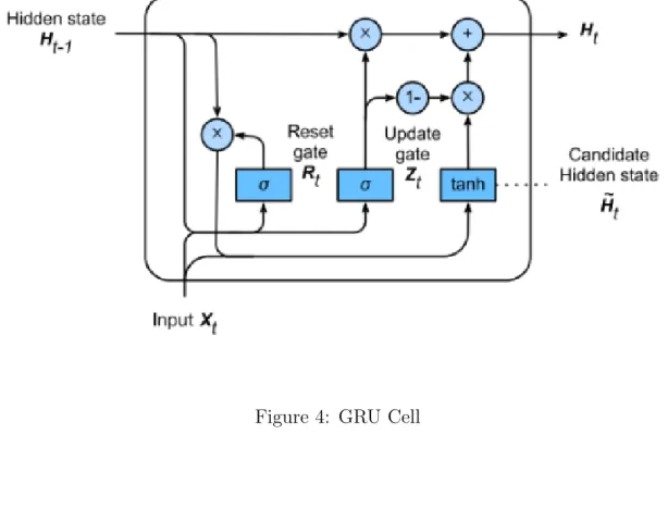
Figure 4: GRU Cell
2.5.2 GRU
GRU (Fig. 4) is similar to LSTM in functionality; it has 2 gates - the “reset” gate which determines how much of the past should be considered, and the “update” gate which determines the attention tradeoff between the current candidate-state and the previous state (Cho, van Merrienboer, Bahdanau, & Bengio, 2014). GRU is computationally more efficient than LSTM, and researchers usually evaluate both units’ performances on sequential mod-elling tasks. This work uses a specialized extension of the GRU called the GRU-Decay (Che, Purushotham, Cho, Sontag, & Liu, 2018).
2.6 Machine Learning in IBD Research
Researchers have used machine learning (ML) to further our understanding of IBD and to guide clinical care. (Wei et al., 2013) predict the genetic risk of CD and UC in a genome-wide
association study using traditional ML models. (Yazdani et al., 2016) project to identify dif-ferences in gut microbiomes of healthy and disease states heavily relied on the Random Forest algorithm. (Mahapatra et al., 2013) segment CD-affected tissues in MRI scans using graph cuts and Random Forest classifiers. (Mossotto et al., 2017) used a combination of supervised and unsupervised learning on endoscopic and histological data; they used unsupervised meth-ods to reduce dimensionality and obtain clusters identifying phenotypes (CD/UC) of IBD in the data, and trained a SVM (support vector machine) classifier to predict the phenotype. (Waljee et al., 2017) trained Random Forest models to forecast IBD-related hospitalizations and steroid use based on aggregates of previous histories.
3.0 Prior Work and Motivation
As part of a preliminary study, I trained various ML models to classify a patient as High-Cost (<$100,000/year) or not, based on the same IBD patient registry dataset (Anderson et al., 2016) used here. After cleaning and preprocessing, I created three representations of the registry dataset. The first dataset maintained the data in their originally recorded format (continuous values). In the second dataset, all numerical features were discretized into categorical labels according to clinical guidelines. In the third dataset, created primarily for training an ANN, each feature was represented as a set of binary dummy variables. Finally, all the observations per patient were aggregated into a single entry. A suite of algorithms - Gradient Boosted Trees, SVM, Tree-Augmented Networks, and a Feed Forward Neural Network - were trained on these aggregated datasets to classify the patient into a utilization phenotype. I obtained an accuracy of 0.89 and an AUROC of 0.748, with features relating to lab results and clinician encounters being most indicative of future charges. To the best of my knowledge, there is no system that models the sequential changes in an IBD patient’s state to predict future IBD-related outcomes. One critical limitation of modelling aggregate clinical data is that they do not take into account the temporal nature of patient treatment trajectories. However, the classification results were strong enough to suggest support for ML approaches to analyze IBD patients in this registry.
To better capture the intertemporal dynamics, the problem requires to be modelled as a multivariate time series. The motivation to use RNNs comes from recent research applying deep recurrent networks to sequential data in the clinical domain. These algorithms are well-suited for large datasets with many features, and the typical size of clinical datasets in the literature are in the order of several hundred thousand to over a few million observations (Johnson et al., 2016) (Ho, Ledbetter, Aczon, & Wetzel, 2017). The dataset used in this study is much smaller in comparison (218,000 observations), and this poses a different set of challenges for effectively modelling the latent distribution in the samples without overfitting to modal patterns. This work incorporates multitask learning that has its roots in clinical prediction (Caruana, Baluja, & Mitchell, 1995).
4.0 Data Description
This work uses a research registry of IBD patients collected at the University of Pitts-burgh Medical Center (UPMC) tertiary care center for digestive disorders. The registry contains datasets of timestamped clinical events such as pathological lab results, active drug prescriptions, diagnostic and surgical procedures, encounters with care providers, Quality-of-Life survey responses, and billing data. These events were merged into longitudinal sequences with 53 dynamic variables for each patient. The sequences are resampled to a monthly rate and the total measurements are recorded in each monthly window. To prevent confounding the model, patients being treated for cancer and/or who had a transplant are excluded. This results in a final population of 2390 patients who have treatment courses ranging from 32 months to 11 years. The data has an average sparsity of around 78%.
4.1 Features
This section presents the clinical features used as predictors to train the model.
4.1.1 Drug Prescriptions
The following categories of prescription drugs are commonly used in IBD treatment: • 5-aminosalicylic acid (5-ASA)
• Systemic Steroids • Immunomodulators • TNF Inhibitors
• Antil-Interleukin-12 antibodies • Anti-Integrin antibodies
• Vitamin D supplements, and • Psychotherapeutic drugs
Each class of drugs pertains to a specific need in the patient. Some drugs are prescribed only in extenuating circumstances. Therefore, this data holds important information about the physician’s estimate of the patient’s current state. The choice to include Psychiatric drugs was made because IBD is known to affect patients’ well-being and quality of life, and a number of studies have attempted (Cawthorpe, 2015) to estimate the relationship between mental health and IBD.
Information about active prescriptions is encoded as a binary variable for each patient-month.
4.1.2 Clinical Lab Results
A physician might prescribe specific lab tests if they suspect those values to be abnormal. Typical lab tests conducted for an IBD patient are:
• 5-Eosinophils (EOS) (Click, Anderson, et al., 2017) • Monocytes (Cherfane et al., 2016)
• Albumin (Koutroubakis, Regueiro, et al., 2016)
• Hemoglobin (Koutroubakis, Ramos-Rivers, et al., 2016) • Erythrocyte Sedimentation Rate (ESR)
• C-Reactive Protein (CRP), and • Vitamin D (Kabbani et al., 2016)
Different lab testing sites use non-standard units. To counter this hetereogeneity, each lab is one-hot encoded for ‘Low’, ‘Normal’ or ‘High’ based on clinically-defined ranges, and the results are summed up for each patient-month.
4.1.3 Diagnostic Procedures
The following gastrointestinal diagnostic tests were included in the dataset: • Colonsocopies
• Endoscopies • Sigmoidoscopies
• Ileoscopies • Anoscopies
• Abdomen/Pelvis CT Scans
The total number of each of these diagnostics in a patient-month is recorded.
4.1.4 Surgeries
The number and frequency of gastrointestinal (GI) surgical procedures is a strong clinical predictor of disease severity (Limsrivilai et al., 2017). Prominent surgeries are colectomies, resections, fistulas and abscesses. All GI surgeries are totaled in each patient-month.
4.1.5 Clinician Encounters
The number of encounters a patient has with their healthcare provider is important information, especially if there is a sudden rise or dip in the frequency (Ramos–Rivers et al., 2014). Encounters are grouped by the channels used - telephone, email or office visits. Encounters at non-GI departments are retained in the dataset, but their counts are stored in a separate variable.
4.1.6 Disease Descriptors
Although Crohn’s Disease and Ulcerative Colitis are collectively termed as IBD, both conditions have differences in symptoms and treatment pathways. Instead of training a separate model, I include a binary flag indicating the disease type. The Harvey Bradshaw (HB) Questionnaire is a survey measuring IBD patients’ quality of life and well-being. More than 2000 patients had at least one response ever. Clinical research suggest the HB Index is a good approximator for disease severity. (Vermeire et al., 2010). Age of Diagnosis is included as some studies suggest a difference in disease phenotype and natural history according to the age of onset (Quezada, Steinberger, & Cross, 2012).
4.1.7 Charges
Clinical researchers helped to identify billed procedures that were related to IBD. I retained the unrelated procedures and their charges in a separate variable as a proxy for the patient’s comorbidities. All charges were inflation-adjusted for 2018 (year of the last observation).
4.2 Model Inputs
A patient’s input multivariate time series of length T having D variables is denoted by
Xp = [x
(1)
p , ..., x(pt)] ∈ RT×D where x(t) ∈ RD refers to the observation at time-stamp t. X is normalized to a standard scale of [-0.5, 0.5] to enable faster convergence in training. To regularize the time series, X is resampled to a monthly rate. Doing so however heavily increases sparsity, resulting in 78% of the values ”missing”.
4.2.1 Missingness Metadata
In addition to Xp, the model is fed two other vectors - the observed mask Mp =
[m(1)p , ..., m(pt)] ∈ {0,1}T×D denoting which variables are observed at time step t, and the
last seen interval ∆p = [δ
(1)
p , ..., δp(t)] ∈ RT×D denoting how long ago from time step t were the variables last observed.
4.2.2 Patient Time Series
Given a patient’s historyHp overM months, a sliding window is used to obtain
overlap-ping training examples with a look-back period b and look-forward period f, such that the
i-th example pair (X(i), Y(i)) is given by (H
p,i:b+i,, Hp,b+i:f+i,). The target labels extracted
fromY(i) (for the period f) are: • annualized total charges • lab results
• diagnostics tests conducted • total surgeries conducted
5.0 Methods
This work investigates if a deep network can learn to adequately represent a temporal se-quence as a single vector. Casting this problem as a multi-class multi-label forecasting task — given a patient’s time series data D = [X, M,∆], predict the labels Lcharge, Llab, Ldiag, Lsurg
— it is possible to test how much information about the future does this representation hold. The proposed model consists of two major blocks - the RNN encoder, which derives an abstract representation of the time series, and the classifiers which predict a label.
5.1 Cross Validation for Time Series
Cross-validation (CV) is a popular and important technique for identifying optimal hy-perparameters and providing robust measurements of model performance. Two popular cross-validation methods arek-fold andholdout cross-validation. For this study that involves a small dataset of clinical time series, various data splitting schemes come with different caveats (Bergmeir & Ben´ıtez, 2012) (Sherman, Gurm, Balis, Owens, & Wiens, 2017). The following sections elaborate on the splitting methodologies and the constraints associated with them.
5.1.1 Naive K-fold Split
In K-fold CV, the dataset is randomly split into K different test sets, and for each set the model is trained on the remaining data. The model is then evaluated by sampling performance scores from allK sets. Such a split ensures that the model is trained and tested on samples that are most representative of the clinical time series.
A significant drawback of this is a risk of information leak between the train and test sets. The random split does not take the chronology of events into consideration, and the training set may contain later observations than the ones in the test set. As verified in this
work, this data leakage trains models that have excellent cross-validation and test scores, but performs poorly on a holdout set of unseen patients.
5.1.2 Chronological Holdout
To overcome these integrity violations, the latter parts of each patient’s time series is held out, and the model is trained only on the former observations. This upholds validation integrity, but at the cost of informativeness. In the IBD time series, clinical events do not follow a general monotonic trend that can be approximated by a model. Events of interest like spikes in abnormal CRP levels or an intensive surgery can occur anywhere in the time series. Given a sufficiently large sample, the model may better approximate the population function from a chronologically-split training set, but it is more difficult to do so from a small esoteric sample.
Moreover, for large look-back b and look-forward f periods, this technique reduces the number of usable observations. Consider a patient whose total duration spans 60 months. Assuming a training set size of 80%, the test size of this patient then contains 12 months. It is not possible to generate test examples for any b+f >12. To use this cross-validation method, the b and f must be small enough to accommodate a representative test set, while still being clinically useful. In the experiments, I use a chronologically held-out set ofb = 24,
f = 8, and a training size of 60%
5.1.3 Chronological Split with Overlap
This scheme refers to a trade-off between the Naive Split that favours representativeness over small data but allows information to leak, and the Chronological Holdout that upholds validation integrity but cannot be used on small datasets. Here the chronological train-test split is not conducted on the patients’ time series, but on the sliding window sequences generated from the time series. There is a minor information leak here: some observations will be a member of both the latter sequences in the training set, and the initial sequences of the validation set. However this may be an acceptable compromise, as the training set is not privy to the target labels in the validation set. Moreover the chronological overlap of
the training and test set is much lesser (because of the intermediate validation set), allowing an honest evaluation of the model in real-world scenarios. In the experiments, I use this splitting scheme for b = 24 and f = 8, with a training size of 80% instead of 60%.
5.2 Model
5.2.1 Encoder
The encoder block of the model consists of L stacked GRU-D layers having 6D hidden memory units each, whereD is the number of input dimensions. In the following equations,
h(lt) represents the hidden state at layerl, andh(l−t)1 is the output of the previous layer at the same time step (or x(t) if l = 0). h(t−1)
l is the output of the same layer from the previous
time step (or a zero-vector when t= 1).
γl(t)= exp{ −max(0,Wlδ(t)+bγ)} (5.1) x(decayt) =m(t)x(t)+ (1−m(t))(γx(t)x(t0)+ (1−γx(t))x˜) (5.2) ˆ x(lt) ={ x (t) decay, ifl = 1 h(l−t)1, ifl >1 (5.3) ˆ hl(t−1) =γh(t)h(lt−1) (5.4) GRU-D decays the inputs to emulate homeostasis when it encounters missing values. The cell learns vectors of decay rates γx and γh at each time step (Equation 5.1). At the first layer, missing values in the input x(t) are replaced by a convex combination of the last observed value x(t0)(t0 < t) and theempirical mean x˜for each variable. Inputs to subsequent layers are not modified (Equations 5.2 - 5.3). The hidden state from the previous time step h(t−1) is also decayed (the authors of the GRU-D paper suggest this captures richer information of missingness directly into the encoded representation).
The decayed input and hidden state are then used to compute the new hidden state h(t)
according to the standard GRU gates:
r(t) =σ(Wrxˆ(t)+Urˆh(t−1)+Vrm(t)+br) (5.5)
z(t) =σ(Wzxˆ(t)+Uzhˆ(t−1)+Vzm(t)+bz) (5.6)
˜
h(t) = tanh(Wxˆ(t)+U(r(t)ˆh(t−1)) +V m(t)+b) (5.7)
h(t)= (1−z(t))hˆ(t−1)+z(t)˜h(t) (5.8) The hidden state of the final layer h(LT) is the abstract representation that is used to classify the input sequence.
5.2.2 Classifier
The model consists of 4 classifiers to predict the charges, diagnostics, lab results, and surgeries in the look-forward period. Each classifier is made up of 3 fully-connected (FC) lay-ers with a Leaky ReLU activation between them. To reduce the risk of vanishing/exploding gradients and facilitate faster convergence, the network uses Xavier weight initialization.
5.2.2.1 Activation Functions Activation functions are typically non-linear and enable the network to learn non-linear approximations of the data. Each FC layer is a linear trans-form of its inputs; the result of stacking multiple linear layers is therefore simply another single linear transform with different parameters. Non-linear activations interspersed be-tween linear FC layers enable the model to generalize over comples phenomena.
The Rectified Linear Unit or ReLU y=max(0, a) is a non-linear activation function that is applied to a neuron output a = WTx+b. ReLU is popular in many deep networks for
its simplicity and effectiveness. The ReLU’s slope is always 0 for non-positive inputs, and 1 otherwise. While this appears to be a limited type of non-linearity, the combined activations
across many neurons (and their various biases) enables the network to model highly complex non-linearities in a computationally efficient manner.
ReLU is usually more robust to vanishing gradients than tanh and sigmoid activations. However, in case all the neuron outputs are negative, the ReLU gradients will be zero and training stagnates - giving rise to the ”dying ReLU” problem. Leaky ReLU solves for this by allowing negative inputs to have a very small non-zero output, thus ensuring that the neuron activation is always non-zero for non-zero inputs.
5.2.3 Regularization
A model with a large number of free parameters can fit to an exceedingly wide range of phenomena. The architecture described above has well over a million! In the absence of larger datasets, a large and eager model is apt to mistake noise or peculiarities as valid signals.
Typical regularization methods in deep learning are weight decay and dropout. Weight decay appends a term (usually the L1 or L2 norm) to the network’s loss function; this reduces neuron weights in proportion to the network’s complexity and a training hyperpa-rameter. Dropout is a more radical approach specific to neural networks, where the network randomly and temporarily shuts down some of the neurons during training. Compensating for their absence, the remaining neurons are ”forced to learn robust features that are useful in conjuction with a random subset of neurons” (Krizhevsky, Sutskever, & Hinton, 2017).
There is no clear science to non-empirically determine the best regularization approach. While it is possible to include both weight decay and dropout, the models in this work use only dropout.
5.2.4 Multitask Learning
Each of the 4 classification tasks has an associated prediction loss that is backpropagated through the model. The output of the classifiers is alogit, or the log of the probabilities for each of the target classes.
5.2.4.1 Charges Predicting the likely inpatient charges s to be incurred by a patient is this model’s primary task. To simplify the task, it is treated as a classification problem by discretizing the annualized charges as
ychg = Low, if s f ×12<$10,000 Mid, if $10,000 ≤ s f ×12<$80,000 High, if s f ×12≥$80,000
Figure 5: Histogram of annual charges
The boundaries for each of the classes was determined after consulting with clinicians and observing the data (Figure 5). TheC = 3 target classes are mutually exclusive with only a single correct class c per example. The classifier’s logits are passed to a softmax function to obtain the predicted probabilitiesyˆfor each class. The loss for the task is thecategorical cross-entropy loss averaged over N examples.
Lchg =− 1 N X log e ˆ yc PC eyj !
5.2.4.2 Diagnostics, Labs, Surgeries Along with learning to predict charges, the model also forecasts on these auxiliary tasks in a bid to learn well-rounded representa-tions of the clinical time series. The training vector yaux ∈ {0,1}15 indicates if either of the 8 diagnostics, 6 labs or a surgery was conducted in the look-forward period. Since they are not mutually exclusive, the logits for each of these are passed to a sigmoid function to obtain their independent probabilities. The loss for is the average binary log loss over all N examples.
Laux =−
1
N
X
[yaux·log(yˆaux) + (1−yaux)·log(1−yˆaux)]
5.2.4.3 Replicated Targets This technique involves having the model make a predic-tion about the charges at every intermediate step in the time series. Lipton et. al suggest capturing local error signals to overcome the problem of backpropagating the error across time. They also use linear scaling to increase the weights of errors made towards the end of the time series. However it is not immediately clear if recent events in the IBD time series are more predictive than earlier events. Hence errors at all steps are weighted equally, and the loss is the average log loss over all T time steps.
Ltr =− 1 N 1 T X N X T log e ˆ yc PC j eyj !
Losses Lchg, Laux, and Ltr are combined by taking their weighted average:
L = αchg·Lchg+αaux·Laux+αtr·Ltr
αchg+αaux+αtr
where α∈ [0,1] is a hyperparameter that determines the relative importance of each task’s error.
5.3 Experiments
I attempt to investigate the ability of deep networks to model clinical time series data with different architectures and dataset splits. The following sections elaborate on the variations tested, the evaluation methodology and results.
5.3.1 Time Horizons
The set of examples for a patient p with a total treatment duration N contains the overlapping sequences with a look-back period of b months and look-forward period of f
months is given by:
Xp ={(Hp(0:b), y (b:f) chg|p),(H (1:b+1) p , y (b+1:f+1) chg|p ), ..., (H (N−b−f:N−f+1) p , y (N−f+1:N) chg|p )}
The values of b and f determine the number of overlapping examples obtainable from the dataset. Smaller values result in a larger number of training samples — beneficial for training models with adequate validation — but are unable to capture the long-term chronicity of IBD. A reasonable midway was considered to be b = 24 and f = 8, which is used in the experiments.
5.3.2 Multitask Loss
For an investigation into the multitask learning effects, the following variations are re-ported:
1. No multitask learning (αaux = 0 andαtr = 0)
2. Auxiliary training without Target Replication (αaux = 0.5 and αtr = 0)
3. Target Replication without Auxiliary training (αaux = 0 andαtr = 0.5)
4. Complete multitask learning (αaux = 1 andαtr = 1)
Their effects are noted by comparing the training and validation losses during training. It is expected that multitask learning will have an implicit regularizing effect.
5.3.3 Architectures
All the models trained in these experiments use 2 stacked GRU-D layers with 312 memory units each, and 3 fully-connected layers. This model includes dropout with probability
p = 50% after each GRU-D layer and p = 30% after each fully-connected layer. It does not use weight decay. A shallow network containing 1 GRU-D layer & 2 fully-connected layers was unable to learn the data and was outperformed by the deep models as well as the baselines.
5.3.4 Baseline
Baselines are well-understood models that provide a point of reference for performance. To provide a minimum baseline, I report the performance of logistic regression, which is widely used in clinical research. A stronger baseline that is more closely related to the deep network is a multilayer perceptron with 3 layers of 312 hidden units, Leaky ReLU activation and 50% dropout. Hyperparameters are chosen from cross-validation, and the MLP is trained for 100 epochs. Both baseline algorithms accept only fixed-size inputs, therefore each sequential input is averaged into one observation before feeding to the baseline classifier.
5.3.5 Evaluation Metrics
Commonly-used classification metrics like accuracy and Area Under the ROC Curve are inadequate to explain a classifier’s performance on imbalanced datasets. The data used in these experiments is extremely skewed; 87% of the samples have a label of Low. A base rate classifier that makes random predictions according to this distribution would have an accuracy of over 60%. A model that only predicts the majority class will obtain an accuracy of 87% - high, but very misleading.
Since this DSS is intended for clinical use, it is important to consider the reliability of the model’s predictions. A few metrics that measure these are Log Loss (lower is better), Cohen’s Kappa (higher is better), Matthews Correlation Coefficient (higher is better), Brier Loss (lower is better). Kappa is a coefficient of agreement; here it measures how much better are the model’s predictions than a base rate classifier. A pitfall of the Kappa is that it is dependent on how the probability of chance in the base rate is defined. A more informative and less biased metric is the Matthews Correlation Coefficient (MCC) which simply computes the correlation coeffecient between the true and predicted labels (Chicco & Jurman, 2020). Therefore this value is high only when the model achieves good results in all four confusion matrix categories. The possible values range from [−1,1] and should be interpreted similar to the correlation coeffecient.
Area Under the Precision-Recall Curve (AUPRC) as a single-point estimate of ability to predict sequences as HC. An ideal DSS should have high precision and recall but in the real-world there is a tradeoff between the two. I report the observed recall at specific levels of precision of 0.4 (R@P=0.4).
These metrics are useful to compare different models’ performances, but are insufficient to evaluate a model in the real-world. A more fair comparison might involve clinical ex-perts providing their predictions given only the data seen by the model. This is however prohibitively expensive and the manual effort needed is difficult to justify.
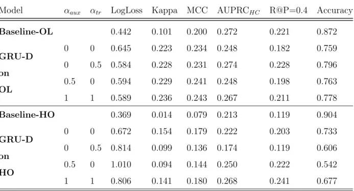
5.4 Results
This section presents the evaluation results of 8 GRU-D models and 2 baseline Multi-layer Perceptrons models. The 4 variations of multitask loss coefficients and both baselines (described in Section 5.3.2) are trained and tested on the Chronological Holdout (HO) and Chronological Overlap (OL) data splits. I don’t report results of the Logistic Regression baseline as it only predicted the majority class for the entire test case.
Both baseline models bias their predictions to Low-Charge; Baseline-OLpredicts 90% of the 2,192 High-Charge sequences as Low-Charge. In comparison, the best performing GRU-D-OL model (αaux = 1, αtr = 1) has a recall of 34% on the High-Charge patients, and
predicts another 32% as Mid-Charge (Appendix A) .
Among the GRU-D models, there is no clearly dominating performance in Table 5.4; from the metrics, it is unclear how multitask learning and target replication are contributing to model performance. However it must be noted that the GRU-D models are trained only on 50 epochs for this experiment; these are probably not enough runs for the complex model to fit all million of its parameters to the data.
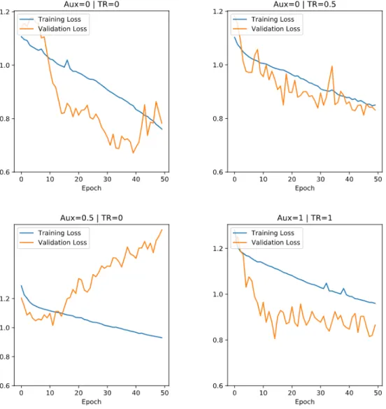
Plotting the training and validation loss lends some insight into the regularization prop-erties of multitask learning (Appendix B). For αtr >0 the validation loss drops in tandem
Model αaux αtr LogLoss Kappa MCC AUPRCHC R@P=0.4 Accuracy Baseline-OL 0.442 0.101 0.200 0.272 0.221 0.872 GRU-D on OL 0 0 0.645 0.223 0.234 0.248 0.182 0.759 0 0.5 0.584 0.228 0.231 0.274 0.228 0.796 0.5 0 0.594 0.229 0.241 0.248 0.198 0.763 1 1 0.589 0.236 0.243 0.267 0.211 0.778 Baseline-HO 0.369 0.014 0.079 0.213 0.119 0.904 GRU-D on HO 0 0 0.672 0.154 0.179 0.222 0.203 0.733 0 0.5 0.814 0.099 0.136 0.174 0.119 0.606 0.5 0 1.010 0.094 0.144 0.250 0.222 0.542 1 1 0.806 0.141 0.180 0.268 0.241 0.677
6.0 Conclusion
In this work, I have explored methods to make the IBD EHR data suitable for training a DNN. The chronic nature of IBD means clinical events can occur irregularly in a patient’s lifecycle. Typical approaches include aggregating past observations or hand-engineering fea-tures describing some temporal characteristics. In consultation with clinical experts and practitioners, I cleaned, processed and feature-engineered unstructured EHR data. I built the data pipeline to transform the raw contents of the EHR database to inputs for a neural network.
One hypothesis that I sought to explore in this work is if the irregularities in medical histories hold useful information. I appended these inputs with metadata about its missing variables, specifically about which ones were missing, and how long they have been missing since. I implemented a specialized GRU-D cell to learn the missingness patterns from the metadata, and built a neural architecture to learn a sequence of clinical events.
I trained the model to primarily predict the healthcare utilization, and on secondary objectives of clinical importance, in an approach called multitask learning. I varied the importances of the secondary objectives relative to the main task, and report their impact on model performance. I reported the classification scorecard of each model, and a the performance of a strong baseline classifier.
In the results I did not find conclusive evidence for multitask learning contributing to well-rounded abstract representations; one reason for this could be that the models were trained only for 50 epochs (models of this scale are usually trained for several hundred epochs) and were not able to learn deeper patterns in the data yet. That said, it is clear that models which learn to perform on multiple tasks simultaneously have a stable training progress; performance on the validation set is similar to that on the training set. This makes intuitive sense because the model tries to approximate an overall distribution instead of latching on to a possibly spurious pattern that only exists in the training dataset. Future experiments should have the model train for more epochs before testing.
a highly imbalanced dataset, and performs better than the baseline on the metrics evaluat-ing classification performance across minor and major classes. However, this performance measure is relative to other classifier models, and may not absolutely capture the systemic biases present in all the classifiers. More work needs to be done to test the clinical efficacy of deep networks to IBD EHR analysis.
6.1 Future Work
More robust experimentation is required to conclusively confirm or dismiss the contribu-tion of secondary tasks and replicacontribu-tion targets to model efficacy. Not only is it important to test the model over a larger number of epochs and varying look-back and look-forward time frames, but it is also necessary to ensure that the data for the secondary tasks are pertinent to the primary objective. In this work, the secondary tasks are to predict if a clinical event occurred in the period in question or not. While this task is simple to engineer in the network architecture, it might be too simplistic for the model to learn anything meaningful about the current input sequence. Future work could consider including more nuanced tasks to allow the model to learn aspects of the patient history clinicians might themselves look for, while attempting a prognostication.
Clinician notes are a rich source of information that lays untapped in the IBD registry. With the current advances in Natural Language Processing and Entity Recognition, these notes could be a treasure for phenotyping a time slice of the patient’s treatment cycle. Extracting meaningful features is an active area of research.
Lastly, future work in this direction will greatly benefit from augmenting the registry dataset, with similar variables from a different population. Since response to IBD treatments is widely variant across individuals, It is difficult to say if the registry dataset has enough information to be representative of all patterns. The registry is maintained for patients in a geographically co-located healthcare network, giving rise to the possibility of systemic biases. Ideally, the augmented data should come from a demographic that is dissimilar to what we currently have in the registry.
Appendix A Confusion Matrices 27708 0 56 2002 0 59 1955 0 237
Confusion Matrix for Baseline-OL
20395 0 1 769 0 3 1389 0 16
Confusion Matrix for Baseline-HO
Figure 6: Baseline Confusion Matrices
23657 2927 1180 1128 620 313 954 588 650
Confusion Matrix for GRUD-OL with
αaux = 1, αtr = 1 15799 2016 2581 401 154 217 580 225 600
Confusion Matrix for GRUD-HO with
αaux = 0, αtr = 0
Appendix B
Loss Trends During Training
Figure 9: Training and Validation Loss Trend (50 epochs) - HO Data Split
References
Abraham, C., & Cho, J. H. (2009). Mechanisms of disease. N Engl J Med,361.
Ali, J. (1994). Neural Networks: A New Tool for the Petroleum Industry? In Euro-pean petroleum computer conference. Society of Petroleum Engineers. Retrieved from
http://www.onepetro.org/doi/10.2118/27561-MS doi: 10.2118/27561-MS
Anderson, A. J. M., Click, B., Ramos-Rivers, C., Babichenko, D., Koutroubakis, I. E., Hartman, D. J., . . . Binion, D. G. (2016, September). Development of an inflammatory bowel disease research registry derived from observational electronic health record data for comprehensive clinical phenotyping. Digestive Diseases and Sciences,61(11), 3236– 3245. Retrieved from https://doi.org/10.1007/s10620-016-4278-z doi: 10.1007/ s10620-016-4278-z
Bates, D. W. (1998, October). Effect of computerized physician order entry and a team in-tervention on prevention of serious medication errors. JAMA,280(15), 1311. Retrieved
fromhttps://doi.org/10.1001/jama.280.15.1311 doi: 10.1001/jama.280.15.1311
Bergmeir, C., & Ben´ıtez, J. M. (2012, May). On the use of cross-validation for time series predictor evaluation. Information Sciences, 191, 192–213. Retrieved from https://
doi.org/10.1016/j.ins.2011.12.028 doi: 10.1016/j.ins.2011.12.028
Bright, T. J., Wong, A., Dhurjati, R., Bristow, E., Bastian, L., Coeytaux, R. R., . . . Lobach, D. (2012, July). Effect of clinical decision-support systems. Annals of Internal Medicine,
157(1), 29. Retrieved from https://doi.org/10.7326/0003-4819-157-1-201207030
-00450 doi: 10.7326/0003-4819-157-1-201207030-00450
Caruana, R., Baluja, S., & Mitchell, T. (1995). Using the future to “sort out” the present: Rankprop and multitask learning for medical risk evaluation. In Proceedings of the 8th International Conference on Neural Information Processing Systems (p. 959–965). Cambridge, MA, USA: MIT Press.
Cawthorpe, D. (2015, February). Temporal comorbidity of mental disorder and ulcerative colitis. The Permanente Journal, 52–57. Retrieved from https://doi.org/10.7812/
tpp/14-120 doi: 10.7812/tpp/14-120
Che, Z., Purushotham, S., Cho, K., Sontag, D., & Liu, Y. (2018, April). Recur-rent neural networks for multivariate time series with missing values. Scientific Re-ports, 8(1). Retrieved from https://doi.org/10.1038/s41598-018-24271-9 doi: 10.1038/s41598-018-24271-9
Cherfane, C., Anderson, A. J., Rivers, C. R., Schwartz, M., Barrie, A., Hashash, J. G., . . . Binion, D. G. (2016, April). 165 Is Monocytosis a Biomarker of Severity in In-flammatory Bowel Disease? Analysis of a 6 Year, Prospective Natural History Reg-istry. Gastroenterology, 150(4), S42. Retrieved from https://doi.org/10.1016/
s0016-5085(16)30266-9 doi: 10.1016/s0016-5085(16)30266-9
Chicco, D., & Jurman, G. (2020, January). The advantages of the Matthews correlation coef-ficient (MCC) over F1 score and accuracy in binary classification evaluation. BMC Ge-nomics, 21(1). Retrieved from https://doi.org/10.1186/s12864-019-6413-7 doi: 10.1186/s12864-019-6413-7
Cho, K., van Merrienboer, B., Bahdanau, D., & Bengio, Y. (2014). On the Proper-ties of Neural Machine Translation: Encoder-Decoder Approaches. arXiv preprint arXiv:1409.1259.
Choi, E., Bahadori, M. T., Schuetz, A., Stewart, W. F., & Sun, J. (2016, 18–19 Aug). Doctor AI: Predicting Clinical Events via Recurrent Neural Networks. In F. Doshi-Velez, J. Fackler, D. Kale, B. Wallace, & J. Wiens (Eds.),Proceedings of the 1st Machine Learning for Healthcare Conference (Vol. 56, pp. 301–318). Children’s Hospital LA, Los Angeles, CA, USA: PMLR. Retrieved from http://proceedings.mlr.press/v56/ Choi16.html
Click, B., Anderson, A. M., Koutroubakis, I. E., Rivers, C. R., Babichenko, D., Machicado, J. D., . . . Binion, D. G. (2017, December). Peripheral eosinophilia in patients with inflammatory bowel disease defines an aggressive disease phenotype. American Journal of Gastroenterology, 112(12), 1849–1858. Retrieved from https://doi.org/10.1038/
ajg.2017.402 doi: 10.1038/ajg.2017.402
Click, B., Binion, D. G., & Anderson, A. M. (2017, March). Predicting costs of care for patients with inflammatory bowel diseases. Clinical Gastroenterology and Hepatology,
15(3), 393–395. Retrieved fromhttps://doi.org/10.1016/j.cgh.2016.11.027 doi: 10.1016/j.cgh.2016.11.027
Cohen, R. D., Larson, L. R., Roth, J. M., Becker, R. V., & Mummert, L. L. (2000, February). The cost of hospitalization in Crohn’s disease. The American Jour-nal of Gastroenterology, 95(2), 524–530. Retrieved from https://doi.org/10.1111/
j.1572-0241.2000.01779.x doi: 10.1111/j.1572-0241.2000.01779.x
Escobar, G. J., Puopolo, K. M., Wi, S., Turk, B. J., Kuzniewicz, M. W., Walsh, E. M., . . . Draper, D. (2013, December). Stratification of risk of early-onset sepsis in newborns ≥34 weeks’ gestation. Pediatrics, 133(1), 30–36. Retrieved from https://doi.org/
10.1542/peds.2013-1689 doi: 10.1542/peds.2013-1689
Esteva, A., Robicquet, A., Ramsundar, B., Kuleshov, V., DePristo, M., Chou, K., . . . Dean, J. (2019, January). A guide to deep learning in healthcare. Nature Medicine, 25(1), 24–29. Retrieved fromhttps://doi.org/10.1038/s41591-018-0316-z doi: 10.1038/ s41591-018-0316-z
Gers, F. A., Schmidhuber, J., & Cummins, F. (1999). Learning to forget: continual prediction with LSTM. In 1999 Ninth International Conference on Artificial Neural Networks ICANN 99. (Conf. Publ. No. 470) (Vol. 2, p. 850-855 vol.2).
Gotz, D., Stavropoulos, H., Sun, J., & Wang, F. (2012). ICDA: a platform for intelligent care delivery analytics. In AMIA Annual Symposium Proceedings (Vol. 2012, p. 264). Gulshan, V., Peng, L., Coram, M., Stumpe, M. C., Wu, D., Narayanaswamy, A., . . . Webster,
D. R. (2016, December). Development and validation of a deep learning algorithm for detection of diabetic retinopathy in retinal fundus photographs. JAMA, 316(22), 2402. Retrieved from https://doi.org/10.1001/jama.2016.17216 doi: 10.1001/ jama.2016.17216
Han, S.-W., Gregory, W., Nylander, D., Tanner, A., Trewby, P., Barton, R., & Welfare, M. (2000, January). The SIBDQ: further validation in ulcerative colitis patients. The American Journal of Gastroenterology, 95(1), 145–151. Retrieved from https://doi
.org/10.1111/j.1572-0241.2000.01676.x doi: 10.1111/j.1572-0241.2000.01676.x
Ho, L. V., Ledbetter, D., Aczon, M., & Wetzel, R. (2017). The dependence of machine learning on electronic medical record quality. In AMIA Annual Symposium Proceedings
(Vol. 2017, p. 883).
Jagannatha, A. N., & Yu, H. (2016). Bidirectional RNN for medical event detection in electronic health records. InProceedings of the 2016 Conference of the North American Chapter of the Association for Computational Linguistics: Human Language Technolo-gies. Association for Computational Linguistics. Retrieved from https://doi.org/
10.18653/v1/n16-1056 doi: 10.18653/v1/n16-1056
Jaspers, M. W., Smeulers, M., Vermeulen, H., & Peute, L. W. (2011). Effects of clinical decision-support systems on practitioner performance and patient outcomes: a synthesis of high-quality systematic review findings. Journal of the American Medical Informatics Association,18(3), 327–334.
Jha, A. K., DesRoches, C. M., Campbell, E. G., Donelan, K., Rao, S. R., Ferris, T. G., . . . Blumenthal, D. (2009, April). Use of Electronic Health Records in U.S. Hospitals. New England Journal of Medicine,360(16), 1628–1638. Retrieved fromhttps://doi.org/
10.1056/nejmsa0900592 doi: 10.1056/nejmsa0900592
Johnson, A. E., Pollard, T. J., Shen, L., wei H. Lehman, L., Feng, M., Ghassemi, M., . . . Mark, R. G. (2016, May). MIMIC-III, a freely accessible critical care database.
Scientific Data,3(1). Retrieved fromhttps://doi.org/10.1038/sdata.2016.35 doi: 10.1038/sdata.2016.35
Jostins, L., , Ripke, S., Weersma, R. K., Duerr, R. H., McGovern, D. P., . . . Cho, J. H. (2012, October). Host–microbe interactions have shaped the genetic architecture of inflammatory bowel disease. Nature, 491(7422), 119–124. Retrieved from https://
doi.org/10.1038/nature11582 doi: 10.1038/nature11582
Kabbani, T. A., Koutroubakis, I. E., Schoen, R. E., Ramos-Rivers, C., Shah, N., Swoger, J., . . . Binion, D. G. (2016, May). Association of vitamin d level with clinical status in in-flammatory bowel disease: A 5-year longitudinal study. American Journal of Gastroen-terology, 111(5), 712–719. Retrieved from https://doi.org/10.1038/ajg.2016.53
doi: 10.1038/ajg.2016.53
Kim, B. S., & Calise, A. J. (1997). Nonlinear flight control using neural networks. Journal of Guidance, Control, and Dynamics, 20(1), 26–33.
Schwartz, M., . . . others (2016). Five-year period prevalence and characteristics of anemia in a large us inflammatory bowel disease cohort. Journal of Clinical Gastroen-terology, 50(8), 638.
Koutroubakis, I. E., Regueiro, M., Schoen, R. E., Ramos-Rivers, C., Hashash, J. G., Schwartz, M., . . . others (2016). Multiyear patterns of serum inflammatory biomarkers and risk of colorectal neoplasia in patients with ulcerative colitis. Inflammatory bowel diseases, 22(1), 100–105.
Krizhevsky, A., Sutskever, I., & Hinton, G. E. (2017, May). Imagenet classification with deep convolutional neural networks. Commun. ACM, 60(6), 84–90. Retrieved from
https://doi.org/10.1145/3065386 doi: 10.1145/3065386
Lasko, T. A., Denny, J. C., & Levy, M. A. (2013). Computational phenotype discovery using unsupervised feature learning over noisy, sparse, and irregular clinical data. PloS one,
8(6).
Limsrivilai, J., Stidham, R. W., Govani, S. M., Waljee, A. K., Huang, W., & Higgins, P. D. (2017). Factors that predict high health care utilization and costs for patients with inflammatory bowel diseases. Clinical Gastroenterology and Hepatology, 15(3), 385– 392.
Lin, J., Keogh, E., Wei, L., & Lonardi, S. (2007). Experiencing SAX: a novel symbolic representation of time series. Data Mining and Knowledge Discovery, 15(2), 107–144. Lipton, Z. C., Kale, D. C., Elkan, C., & Wetzel, R. (2015). Learning to diagnose with LSTM
recurrent neural networks. arXiv preprint arXiv:1511.03677.
Liu, Y., Ge, T., Mathews, K. S., Ji, H., & McGuinness, D. L. (2018). Exploiting task-oriented resources to learn word embeddings for clinical abbreviation expansion. arXiv preprint arXiv:1804.04225.
Mahapatra, D., Schuffler, P. J., Tielbeek, J. A. W., Makanyanga, J. C., Stoker, J., Taylor, S. A., . . . Buhmann, J. M. (2013, December). Automatic detection and segmentation of crohns disease tissues from abdominal MRI. IEEE Transactions on Medical Imaging,
32(12), 2332–2347. Retrieved from https://doi.org/10.1109/tmi.2013.2282124
doi: 10.1109/tmi.2013.2282124
unsuper-vised representation to predict the future of patients from the electronic health records.
Scientific Reports, 6(1). Retrieved from https://doi.org/10.1038/srep26094 doi: 10.1038/srep26094
Miriovsky, B. J., Shulman, L. N., & Abernethy, A. P. (2012). Importance of health in-formation technology, electronic health records, and continuously aggregating data to comparative effectiveness research and learning health care. Journal of Clinical Oncol-ogy,30(34), 4243–4248.
Mossotto, E., Ashton, J. J., Coelho, T., Beattie, R. M., MacArthur, B. D., & Ennis, S. (2017, May). Classification of paediatric inflammatory bowel disease using machine learning. Scientific Reports, 7(1). Retrieved from https://doi.org/10.1038/s41598
-017-02606-2 doi: 10.1038/s41598-017-02606-2
Osheroff, J. A., Teich, J. M., Middleton, B., Steen, E. B., Wright, A., & Detmer, D. E. (2007, March). A roadmap for national action on clinical decision support. Journal of the American Medical Informatics Association, 14(2), 141–145. Retrieved from https://
doi.org/10.1197/jamia.m2334 doi: 10.1197/jamia.m2334
Pomerleau, D. A. (1989). ALVINN: An Autonomous Land Vehicle in a Neural Network. In Advances in Neural Information Processing Systems 1 (p. 305–313). San Francisco, CA, USA: Morgan Kaufmann Publishers Inc.
Pople, H. E., Myers, J. D., & Miller, R. A. (1975). DIALOG: A Model of Diagnostic Logic for Internal Medicine. In Proceedings of the 4th International Joint Conference on Artificial Intelligence - Volume 1 (p. 848–855). San Francisco, CA, USA: Morgan Kaufmann Publishers Inc.
Quezada, S. M., Steinberger, E. K., & Cross, R. K. (2012, August). Association of age at diagnosis and Crohn’s disease phenotype. Age and Ageing, 42(1), 102–106. Retrieved
from https://doi.org/10.1093/ageing/afs107 doi: 10.1093/ageing/afs107
Ramos–Rivers, C., Regueiro, M., Vargas, E. J., Szigethy, E., Schoen, R. E., Dunn, M., . . . Binion, D. G. (2014, June). Association between telephone activity and features of patients with inflammatory bowel disease. Clinical Gastroenterology and Hepatology,
12(6), 986–994.e1. Retrieved from https://doi.org/10.1016/j.cgh.2013.11.015
Rumshisky, A., Ghassemi, M., Naumann, T., Szolovits, P., Castro, V. M., McCoy, T. H., & Perlis, R. H. (2016, October). Predicting early psychiatric readmission with natural language processing of narrative discharge summaries. Translational Psychiatry,6(10), e921–e921. Retrieved from https://doi.org/10.1038/tp.2015.182 doi: 10.1038/ tp.2015.182
Sherman, E., Gurm, H., Balis, U., Owens, S., & Wiens, J. (2017). Leveraging clinical time-series data for prediction: a cautionary tale. In AMIA Annual Symposium Proceedings
(Vol. 2017, p. 1571).
Shickel, B., Tighe, P. J., Bihorac, A., & Rashidi, P. (2018, September). Deep EHR: A survey of recent advances in deep learning techniques for electronic health record (EHR) analysis. IEEE Journal of Biomedical and Health Informatics, 22(5), 1589– 1604. Retrieved from https://doi.org/10.1109/jbhi.2017.2767063 doi: 10.1109/ jbhi.2017.2767063
Silverstein, M. D., Loftus, E. V., Sandborn, W. J., Tremaine, W. J., Feagan, B. G., Nietert, P. J., . . . Zinsmeister, A. R. (1999, July). Clinical course and costs of care for Crohn’s disease: Markov model analysis of a population-based cohort. Gastroenterology,117(1), 49–57. Retrieved from https://doi.org/10.1016/s0016-5085(99)70549-4 doi: 10 .1016/s0016-5085(99)70549-4
Vermeire, S., Schreiber, S., Sandborn, W. J., Dubois, C., & Rutgeerts, P. (2010, April). Correlation Between the Crohn’s Disease Activity and Harvey–Bradshaw Indices in Assessing Crohn’s Disease Severity. Clinical Gastroenterology and Hepatology, 8(4), 357–363. Retrieved from https://doi.org/10.1016/j.cgh.2010.01.001 doi: 10 .1016/j.cgh.2010.01.001
Waljee, A. K., Lipson, R., Wiitala, W. L., Zhang, Y., Liu, B., Zhu, J., . . . Higgins, P. D. R. (2017, December). Predicting hospitalization and outpatient corticosteroid use in in-flammatory bowel disease patients using machine learning. Inflammatory Bowel Dis-eases, 24(1), 45–53. Retrieved from https://doi.org/10.1093/ibd/izx007 doi: 10.1093/ibd/izx007
Wei, Z., Wang, W., Bradfield, J., Li, J., Cardinale, C., Frackelton, E., . . . others (2013). Large sample size, wide variant spectrum, and advanced machine-learning technique
boost risk prediction for inflammatory bowel disease. The American Journal of Human Genetics, 92(6), 1008–1012.
Wharam, J., & Weiner, J. (2012, March). The promise and peril of healthcare forecasting.
American Journal of Managed Care, 18(3), e82–e85.
Yazdani, M., Taylor, B. C., Debelius, J. W., Li, W., Knight, R., & Smarr, L. (2016, December). Using machine learning to identify major shifts in human gut microbiome protein family abundance in disease. In 2016 IEEE International Conference on Big Data (Big Data). IEEE. Retrieved from https://doi.org/10.1109/bigdata.2016