Social desirability bias (SDB) is defined as a tendency in people to present themselves in a more socially acceptable light, when faced with sensitive questions. People with a higher degree of SDB tend to give answers that will make them look good rather than those that are accurate. Randomized Response Technique (RRT) is one of several techniques used by researchers to circumvent social desirability bias in personal interview surveys. Starting from the pioneering work of Warner (1965), many versions of RRT have been developed that can deal with both categorical and quantitative responses. In this thesis we will focus only on those RRT models that are useful for quantitative responses. We will discuss a variety of quantitative RRT models including full, partial and optional RRT models. However, our primary focus in this thesis will be on optional RRT models. Specifically we will compare one-stage optional RRT models with two-stage optional RRT models.
For optional RRT models, both additive and multiplicative RRT models have been used in the literature. However, survey respondents with minimal or no math-ematical background may find additive models easier to handle. In this thesis we will discuss some other advantages of using additive optional RRT models as op-posed to multiplicative optional RRT models. We will develop unbiased estimators for both the mean and the sensitivity level of a quantitative response sensitive ques-tion. We will also try to validate the proposed estimators by way of a simulation study. Throughout this thesis, we will use only the simple random sampling with replacement (SRSWR) design. However, the results can also be extended to other sampling designs.
by Supriti Sehra
A Thesis Submitted to
the Faculty of The Graduate School at The University of North Carolina at Greensboro
in Partial Fulfillment
of the Requirements for the Degree Master of Arts
Greensboro 2008
Approved by
My husband and our families For all their support and encouragement.
This thesis has been approved by the following committee of the Faculty of The Graduate School at The University of North Carolina at Greensboro.
Committee Chair Committee Members
Date of Acceptance by Committee Date of Final Oral Examination
I would like to thank my advisor and committee chair Professor Sat Gupta for all his guidance, support and patience throughout the preparation of this thesis. I would also like to thank thesis committee members Professor Maya Chhetri and Professor Scott Richter for their time and effort in reviewing this work.
Page CHAPTER
I. INTRODUCTION. . . .1
1.1 Background . . . 1
1.2 Circumventing Social Desirability Response Bias . . . 2
1.3 Randomized Response Technique . . . 6
1.4 Goals . . . 9
II. ONE AND TWO-STAGE RANDOMIZED RESPONSE MODELS . . . . 11
2.1 Binary Randomized Response Models . . . 11
2.2 Quantitative Additive Randomized Response Models . . . 16
2.3 Quantitative Multiplicative Randomized Response Models . . . 20
III. OPTIONAL RANDOMIZED RESPONSE MODELS . . . 23
3.1 One-stage Optional Randomized Response Models . . . 23
3.2 Two-stage Optional Randomized Response Models . . . 30
IV. PROPOSED TWO-STAGE OPTIONAL RRT MODELS . . . 35
4.1 Proposed Model 1: Two-stage Multiplicative Optional RRT Model using Two Independent Samples . . . 35
4.2 Proposed Model 2: Two-stage Additive Optional RRT Model using Two Independent Samples . . . 38
V. SIMULATION STUDY AND CONCLUSIONS . . . 47
5.1 Quantitative Additive Optional RRT Models with Optimal Sample Selection . . . 48
5.2 Simulation Results based on Equal Sample Sizes . . . 53
5.3 Concluding Remarks . . . 64
5.4 SAS Code . . . 65
BIBLIOGRAPHY . . . 70
CHAPTER I INTRODUCTION 1.1 Background
One of the classic problems encountered in behavioral and social sciences is estimat-ing the prevalence of a sensitive or delicate behavior. For example, researchers may want tofind out the proportion of people that have cheated on a test in high school, or may want to estimate the number of alcoholic drinks people consume per week. A method that is widely used in the estimation of this type of sensitive behavior often involves conducting some form of a survey. But before the investigators can assert the validity of responses in their survey, they need to overcome a major obstacle: a condition known as “Social Desirability Response Bias.”
In brief, Social Desirability Bias (SDB) can be defined as the bias created due to a person’s desire to be viewed favorably by others. Specifically, individuals have a natural inclination to present themselves in a more positive orsocially acceptable manner to their interviewers, due to their perceived fear of negative consequences. These negative consequences may be concrete punitive actions or something intan-gible like embarrassment, depending on the type of sensitive question being asked. For example, if a sensitive question involves admitting to an illegal behavior, respon-dents may genuinely be afraid of repercussions from the law. By the same token, if the sensitive question entails answering personal health questions, respondents may be embarrassed to reveal their true behavior in fear of negative judgments by the interviewer. Regardless, researchers end up dealing with fabricated or distorted
responses, thus leading to inaccurate or invalid estimates of the sensitive behaviors they are studying. SDB usually presents itself in relation to external environmental situations or internal individual characteristics. External situations may include the effect of who is administering the survey or an item characteristic in terms of “perceived desirability of behavior.” For example, a person may not want to admit to having called in sick to work without being sick. Internal individual attribute relates to differences between individual personality traits in terms of “impression management” or “self-deception” (Randall and Fernandes, 1991). For example, a person may be reluctant to admit that he has a drinking problem, perhaps even to himself, even though clinically he would be diagnosed as an alcoholic.
1.2 Circumventing Social Desirability Response Bias
There have been several techniques explored in the past to cope with SDB. We will briefly outline some of these techniques which include guaranteeing confidentiality, employing the SDB scale, and using the Bogus Pipe Line (BPL) method. Finally, we will describe in detail our chosen method of dealing with SDB: the Randomized Response Technique (RRT).
One of the best ways to elicit truthful responses, and thus minimize SDB, is to guarantee confidentiality. This may not be as simple as the researchers ver-bally assuring the respondents that “your data will only be analyzed in aggregate form, and you cannot be individually identified.” To ensure that respondents will provide the most truthful responses possible, they have to believe that “complete anonymity” from everyone involved in the process actually exists. This is best achieved via a completely anonymous survey, like a mail-in questionnaire with no identifying data, where there is no respondent-to-researcher contact whatsoever. Unfortunately, mail-in surveys have abysmal response rates, thus leading to a
dif-ferent set of problems. Not only will the low response rate affect the precision of results, but the non-responders may fit into their own distinct categories, creating a non-response bias in its own right. On the flipside, in-person surveys have the highest response rates, undoubtedly because it is much more difficult for the respon-dents to refuse participation in a face-to-face situation with the interviewers. But this same face-to-face interaction also makes it more awkward for the respondents to be completely candid with their responses to sensitive questions. In-person studies having the most direct respondent-to-researcher contact, not surprisingly, tend to markedly accentuate SDB and produce the least reliable results.
The method just outlined tries to decrease SDB, where as other methods aim to measure and account for its severity, and then try to make adjustments accordingly during analysis. One such method uses a “SDB scale.” Crowne and Marlowe (1960), developed the Crowne-Marlowe Social Desirability Bias (MCSDB) scale which measures individual SDB levels. A survey which lists 33 personal at-titude type statements is administered to the subjects. The subjects are asked if each statement is true or false for them personally. Each statement has a so-cially accepted or morally “correct” answer, and depending on how the statement is worded, that could be “true” or “false (see example below). A socially correct answer is scored as one point, while an incorrect answer is scored as zero points. Thus the higher the SDB score for the whole survey, the greater the tendency of the individual to give socially desirable responses (or inflate SDB.) Although useful, the MCSDB scale measurement can add significantly to the respondent burden which can lead to lower response rates. To this end, Reynolds (1982) developed compara-ble 11, 12, and 13 item condensed versions of the test. The 13 item version yielded the best results in approximating the original MCSDB scale, and is shown in Table 1.1 below. The socially appropriate or correct answer is listed in parentheses next
to each item. These SDB scores can be used in conjunction with the other ques-tions under investigation to see if there is a significant impact on how individuals answer other questions. If so, the SDB scores can be used as a covariate during the analysis phase of the study, to adjust the means for the sensitive question(s) under investigation.
Table 1.1: Reynolds 13-Point SDB Questionnaire with socially desirable responses shown in parentheses
1 It is sometimes hard for me to go on with my work if I am not encouraged. (F)
2 I sometimes feel resentful when I don’t get my way. (F)
3 On a few occasions, I have given up doing something because I thought too little of my ability. (F)
4 There have been times when I felt like rebelling against people in authority even though I knew they were right. (F)
5 No matter who I’m talking to, I’m always a good listener. (T) 6 There have been occasions when I took advantage of someone.
(F)
7 I’m always willing to admit it when I make a mistake. (T) 8 I sometimes try to get even, rather than forgive and forget. (F) 9 I am always courteous, even to people who are disagreeable. (T) 10 I have never been irked when people expressed ideas very diff
er-ent from my own. (T)
11 There have been times when I was quite jealous of the good fortune of others. (F)
12 I am sometimes irritated by people who ask favors of me. (F) 13 I have never deliberately said something that hurt someone’s
feelings. (T)
Another novel strategy for circumventing SDB is using an experimental method known as the Bogus Pipe Line (BPL) method. Developed by Jones and Sigall (1977), it may be best described as a “fake lie detector test”. Respondents are hooked up to electrodes that supposedly send signals to a device which can detect if the respondent is being truthful or not. During the initial phase of the experiment, respondents are asked to answer some questions, the answers for which
are already known to the investigators. They are encouraged to give some truthful responses, and some that are fabricated, so that the investigators can “prove” to the respondents that the device to which they are attached actually works. Every time an untruthful response is provided, the interviewer presses a hidden buzzer indicating that an untruthful response has been detected. This technique can be quite successful in reducing SDB, since many if not most of the respondents do end up believing that the device is legitimate (Roese, and Jamieson, 1993). However, as with the SDB scale method described earlier, and even more so with this method, a major drawback is that it is extremely resource intensive, not only for the respon-dents, but also for the investigators. A great deal of time and money need to be invested in setting up and running the rather complex experimental conditions and physical machinery. Also, the method is obviously not portable. This method may be best used when the benefits of usage outweigh the large costs involved. Another pertinent philosophical criticism posed against this technique is that the researcher may not be acting in a truly ethical manner in conducting the study, as the re-searcher is essentially deceiving the subject as to the capabilities of the machine used.
One important note about the nature of SDB must be stressed. All the methods that we list in this thesis cannot completely circumvent SDB, they just try to mitigate it. As described earlier, people also have an internal “self-deception” mechanism continually at work, which tries improve their self-esteem. This results in people subconsciously putting themselves in a more positive light without being aware of it.
1.3 Randomized Response Technique
Now we will describe another method for coping with SDB, which will be the main focus of discussion in this thesis. This resourceful method was devised by Warner (1965) to decrease SDB and is called the Randomized Response Technique (RRT). Broadly speaking, while employing this technique, the respondent is asked to ran-domize or “scramble” the response to a sensitive or threatening question. This “scrambling” is based on some preset randomization device. The key point to take notice of here is that the subject’s reported response is based on chance. That is to say, it is based on the outcome of the randomization device, and as a result, the respondent’s “public” answer is “cloaked”. The respondent is convinced that the unscrambling can be done only at the group level and not at the individual level. This allows the respondent to have the anonymity needed to be able to answer freely in a face-to-face situation, thereby helping decrease SDB.
A quick example of a typical RRT set-up will help clarify the technique better. Let’s say we are interested in estimating the “average number of alcoholic drinks consumed daily” in a population. In a regular in-person survey, the interviewer would directly ask the respondent: “how many alcoholic drinks do you consume on a typical day?” This question would make some respondents feel quite uncomfortable, especially in a face-to-face situation with the interviewer, and therefore pressure them into understating or distorting their “true responses.” But in the RRT realm, for the same question, the scenario would be somewhat different. Let’s say we have chosen our randomization device to be a standard deck of cards, with the face cards discarded. The respondent would be given the deck of cards, asked to pick a card, then without letting the interviewer see that card, simply report the sum of the “number listed on the card” and the “true response” back to the interviewer.
give more truthful responses without embarrassment (albeit scrambled responses), is that they can easily see that the interviewers do not know which card they personally picked, and thus cannot know their true responses on an individual level. But an even more interesting aspect about using this method is that, even without knowing the true individual level responses, researchers can calculate group level estimates for the sensitive behavior being studied. This is done using the known distribution properties of the randomization device being employed and other mathematical techniques.
Most RRT models are some variant of the example described above. But all have two things in common: one is the “randomization” feature and the other is the “anonymity” feature — especially in front of the interviewer. This is where the choice of randomization devices becomes important. Randomization devices theoretically can take various forms, for example, a coin, a pair of dice, a deck of cards, a random number generator, or even a roulette wheel. But practically speaking, a randomiza-tion device that is portable, easy to understand and handle for respondents in any RRT experimental environment, would be preferable. More importantly, a random-ization device that easily allows the respondent to hide the outcome of the device from the interviewer would be ideal. A standard or appropriately modified deck of cards fits all the above criteria. Thus in most of the models described in this thesis we will use a deck of cards as our preferred randomization device.
Many types of RRT models have been developed in the past, and they can be categorized as two major types: binary and quantitative. Binary response models are used to estimate theproportion of some behavior or occurrence in a population, and elicit a binary response during the RRT process. For example, to estimate the “proportion of people who drank coffee today” we could list statements: “I drank coffee today” and “I did not drink coffee today” on the cards in a deck.
The respondent would randomly pick a card, and simply respond “true” or “false” to the statement listed on the card. Thus the respondent is not stating explicitly whether or not he drank coffee, he is simply responding to the statement shown on the randomly drawn card. Quantitative response models are used to estimate the mean value of some behavior in a population. They can be further sub-classified as either additive models or multiplicative models. For example, to estimate “average number of cups of coffee consumed daily” we could use a standard deck of cards. The respondent would pick a card, and for the additive model, would respond with the sum of the card value and his true response; while for the multiplicative model, he would respond with the product of the card value and his true response.
RRT models can also be categorized by how the respondents are instructed to randomize. If all respondents are asked to randomize their response, the model is characterized as a “full randomization model.” If some of respondents are instructed to randomize their response, the model is characterized as a “partial randomization model” or a “two-stage model.” And finally, if respondents are given an option to randomize their response, it is characterized as an “optional randomization model.” In connection with the “optional randomization model,” another key concept of “question sensitivity level” needs introduction. “Sensitivity” is defined as the proportion of respondents who think the question is sensitive and hence choose to randomize their responses. Earlier we had specified that in quantitative RRT models, we estimate the mean value for a sensitive behavior. But in an optional randomization model, we end up estimating two parameters: the mean value of the sensitive behavior and the “sensitivity” level of that behavior. RRT models can also be classified as one-stage and two-stage (as indicated above, with the “partial randomization model”. One-stage specifies respondents to follow either the full randomization or optional randomization route in one phase. On the other hand,
“partial randomization models” are like two-stage models, because a proportion of respondents (based on some randomization device) is asked to answer truthfully, while the rest are asked to randomize (again based on some randomization device.) 1.4 Goals
In general, each model described above in progression is better than the one previ-ous to it, in terms of a balance between the model’s relative efficiency (decreased variance) and model’s ease of use in conjunction with the respondent’s perceived anonymity level. Previously, a one-stage optional additive model using two inde-pendent samples (Gupta et al., 2006) and a two-stage optional multiplicative model using one sample (Gupta and Shabbir, 2007) have been specified. Both have their own distinct advantages and disadvantages. We aim to use these two models as a basis, and propose a “two-stage additive optional model using two independent samples” which would optimize the benefits of each, and produce a model with greater efficiency.
In Chapter 2, we will start with the theoretical framework of RRT and de-scribe the methodology involved in various previous models that are relevant for the development of our current models. Namely, we will begin by outlining the basic binary and quantitative response models. In Chapter 3, we will introduce the optional RRT model. We will also compare and contrast the differences among full, partial, and optional quantitative randomization models. Moreover, we will discuss the shortcomings and benefits of additive versus multiplicative models in conjunction with one-stage and two-stage studies. In Chapter 4, we will specify in detail our proposed “two-stage optional additive RRT model using two indepen-dent samples.” In Chapter 5, we will provide simulation results for this model in comparison to other models and also provide some concluding remarks.
We would like to note that there are many other types of RRT models that exist in the literature. However, our focus in this thesis will be on variations of Warner’s (1965) binary response RRT model and the Eichhorn and Hayre (1983) quantitative response model.
CHAPTER II
ONE AND TWO-STAGE RANDOMIZED RESPONSE MODELS
In this chapter we will introduce both binary response and quantitative re-sponse RRT models. First we will outline some binary rere-sponse models, since they form the historical backbone of RRT research. But after that we will concentrate mainly on the quantitative models, since they form the basis of the proposed models in this thesis.
As briefly introduced earlier, binary response models are used in estimating the proportion of some behavior or occurrence in the population. As the name im-plies, there are two mutually exclusive responses possible (‘yes/no”, “agree/disagree”, “true/false” etc.) On the other hand, quantitative response models involve numeric responses. Thus, if we want to estimate the mean of a random variable that de-scribes some behavior or occurrence, we would use a quantitative response model. In the following sections, we will describe in detail the early models developed for these two situations. In conjunction, we will also define and explain the differences between full and partial randomization models, which will come into play when later defining our proposed models.
2.1 Binary Randomized Response Models
2.1.1 Full Binary RRT Model
Most of the RRT models are based on the pioneering work done by Stanley Warner in 1965. Warner’s model is used to estimate the proportion of subjects with a
sensitive behavior or characteristic. In order to estimate this proportion, a ran-domization device such as a deck of flash cards is employed, whereby all subjects are asked to randomize their responses based on the deck of cards. The sampling scheme considered here and throughout this thesis is simple random sampling with replacement. Since all subjects are asked to scramble their responses, the model is called a “full randomization” model. Two types of statements are written on the cards: a certain proportion of cards state “I have characteristic A;” the remaining proportion of the cards state “I do not have characteristic A.” If the subject agrees with the statement on the card that he happens to pick, the response would be “yes.” Conversely, if the subject disagrees with the statement, the response would be “no.” It is important to note, that the interviewer has not seen the card that the respondent has picked, and thus does not know which question is being answered. The interviewer simply records the “yes” or “no” responses.
So mathematically, lettingπ be the true proportion of the subjects with the sensitive characteristic, andpbe the proportion of cards with “I have characteristic A” written on them, the probability of a “yes” response, py, would be
py =pπ+ (1−p) (1−π). (2.1)
Solving for π , we get
π = py −(1−p)
2p−1 , p6=.5 (2.2)
Using the sample data leads to Warner’s unbiased estimator for π given by
b
πw =
b
py −(1−p)
2p−1 . (2.3)
Note the proportion of “yes” responses is estimated by
b
py = n1
where nis the sample size and n1 is the number of “yes” responses. From the fact that
V ar(pby) =
py(1−py)
n , (2.5)
it can be verified that the variance for the estimatorπbw is: V ar(πbw) =
π(1−π)
n +
p(1−p)
n(2p−1)2. (2.6)
The second term in the above equation ³np(2(1p−p) −1)2
´
is the penalty for using the RRT model. Note that this penalty is minimized when p≈0 or p≈1.
For example, if we were interested in estimating the proportion of people who have ever tried cocaine, the following display shows the four possible outcomes for this RRT process. The respondent’s reported response, which is listed in the cells, is based on two factors: his “true cocaine user status” and the “card the respondent he happens to pick”. The “true cocaine user status” is specified in the left margin column, while the “card picked” is specified in the header row. The proportions for each of the two types of cards and the proportions for each of the two types of user status are shown in parentheses
True Status Card Picked
I have tried cocaine(p) I have never tried cocaine(1−p)
User(π) yes no
Non-User(1−π) no yes
Each individual participant would simply answer “yes” or “no” truthfully, based on the card he happens to pick. So if a person who has tried cocaine before picks the “I have tried cocaine” card, he would agree with that statement, so he would simply answer “yes.” On the other hand, if a person who has tried cocaine
picks the “I have never tried cocaine” card, he would disagree with that statement, so he would answer “no.” Using the display, it’s easy to verify the specification for proportion of “yes” responses listed in equation (2.1) above. Note that the proportions p and 1−p are known, as are the number of “yes” responses n1 and the sample size n, hence we can calculate the values ofπbw and V ar(πbw).
2.1.2 Partial Binary RRT Model
Building on Warner’s original model, Mangat and Singh (1990) proposed a slightly different model to increase the efficiency of Warner’s estimator. Rather than having all subjects scramble their response, they proposed a two-stage model. In stage 1, some proportion of the subjects would respond truthfully, while the rest would go to stage 2, whereby they scramble their response (i.e., stage 2 subjects would follow Warner’s model.) Which subjects go to stage 2 is based on a “stage 1 randomization device”. For instance, the “stage 1 randomization device” could be a deck of cards, with a known proportion (T) of cards asking the subject to answer the “I have characteristic A” question truthfully; the remaining proportion (1−T) of cards ask the subject to use the “stage 2 randomization device” to answer the question. All subjects relegated to stage 2 scramble their responses, exactly as they would have with Warner’s full randomization model. Again, the interviewer does not know which question you answered or if you answered in stage 1 or stage 2; he merely records the “yes” or “no” responses.
Updating Warner’s model above, letπbe the true proportion of subjects with the sensitive characteristic, T be the proportion of subjects answering truthfully in stage 1, and p be the proportion of cards in stage 2 with “I have characteristic A” written on them, then the probability of a “yes” response, py, becomes
Using the sample data leads to the Mangat and Singh unbiased estimator for the proportion of sensitive characteristic, given by
b
πms =
b
py−(1−T) (1−p)
(2p−1) + 2T(1−p), (2.8) where pby = nn1, nis the sample size, and n1 is the number of “yes” responses.
The variance for this estimator is given by V ar(πbms) =
π(1−π)
n +
(1−T) (1−p) [1−(1−T) (1−p)]
n[(2p−1) + 2T (1−p)]2 . (2.9) The second term in the equation is the penalty for using this model. Note that when T = 0 this model reduces to Warner’s full RRT model specified above.
So if we use the same example of estimating the proportion of people who have ever tried cocaine, the following display shows all the possible reported re-sponses using the partial RRT model:
True Status Stage 1 Card(T) Stage 2 Card(1−T) Reported Response
User (π) Tell the truth
go to S2 go to S2
N/A
I’ve tried cocaine I’ve never tried cocaine
YES YES NO
Non-User
(1−π)
Tell the truth go to S2 go to S2
N/A
I’ve tried cocaine I’ve never tried cocaine
NO NO YES
Note that the Mangat and Singh partial RRT estimatorπbms is more efficient
than Warner’s full RRT estimator πbw for fixed sample size if T > 1−2p
1−p , which is always true when p > .5.
2.2 Quantitative Additive Randomized Response Models
While the previously described binary response RRT models form a good basis for explaining the intricacies of how RRT models function, we will devote the rest of the thesis to quantitative response RRT models. For quantitative response RRT models we want to estimate the mean prevalence of some sensitive behavior. We will outline the additive models first, since they are easier to comprehend for the respondents and also, mathematically easier to analyze. For the additive quantitative model, subjects would be asked to scramble their responses using a randomization device like a deck of cards. Now, each of the cards in the deck would have a number listed on it, where the numbers in the deck follow a known probability distribution. The subject would be asked to add his “true response” to the “number listed on card” he picked, and then report only the sumto the interviewer. The interviewer cannot see the card picked and would simply record a number.
2.2.1 Full Additive RRT Model
The quantitative additive version of Warner’s binary full randomization model is specified below (Warner, 1971). Again, since it’s a full randomization model, all subjects are instructed to randomize their responses based on a outcome of the randomization device with known mean and variance.
Mathematically, for the additive model, if we letY be the reported response, X be the true sensitive variable of interest with unknown mean μx and unknown
varianceσ2
x, and S be the scrambling variable (independent ofX) with known true
mean μs (E(S) =μs) and knownvariance σs2, then
The expected response is given by
E(Y) = E(X) +E(S)
= μx+μs. (2.11)
Estimating E(Y) by the sample mean Y of the reported responses, we get the unbiased estimator for the mean of the sensitive variable, given by
b
μx =Y −μs. (2.12)
The variance for this estimator is given by V ar(μbx) = V ar ³ Y´= σ 2 y n = σ 2 x n + σs2 n. (2.13) In equation (2.13), σs2
n represents the penalty for using a RRT model.
For example, if researching the average weekly alcohol consumption rate, we may ask the subjects “how many alcoholic drinks do you typically consume per week?” We would ask them to add their true response to the numeric card they pick from the deck. The cards in the deck we created list the numbers 5,6,7,8, and 9 with corresponding frequencies of 6,10,16,10,and 6, respectively. Thus, the frequency distribution of the card values have a mean μs = 7 and variance of 1.42.
If we get the following experimental result corresponding to a sample of size 5,
TRUE # of drinks Card Picked Reported Response
5 9 14 0 7 7 7 5 12 6 6 12 3 6 9 Y= 10.8 b μx=Y−μs= 10.8−7 = 3.8
then our estimate forμx would be 3.8.
2.2.2 Partial Additive RRT Model
Building upon the quantitative full additive RRT model, Gupta and Thornton (2004) have described a partial (two-stage) quantitative randomization model. Sim-ilar to the binary version of the partial randomization model, some known propor-tion (T) of cards in the deck ask subjects to respond truthfully (stage 1), while the remaining proportion (1−T) of cards ask the respondents to report the sum of the number listed on the card and their true response (stage 2).
LetT be the proportion of cards asking respondents to answer truthfully, Y be the reported response, be the sensitive variable of interest with unknown mean
μx and unknownvariance σ2x, andS be the scrambling variable (independent ofX)
with knowntrue mean μs (E(S) =μs) and variance σs2, then Y =
(
X with probability T
X+S with probability (1−T). (2.14) Expected response is given by
E(Y) = (T)E(X) + (1−T)E(X+S) = (T)μx+ (1−T)(μx+μs)
= μx+ (1−T)μs. (2.15)
Substituting the sample mean Y of the reported responses for E(Y), we get the unbiased estimator for the mean of the sensitive variable given by
b
μx =Y −(1−T)μs. (2.16)
The variance for this estimator is given by V ar(μbx) = σ2 x n + (1−T)(σ2 s +Tμ2s) n
= 1 n[σ
2
x+ (1−T)(σ2s+Tμ2s)]. (2.17)
Using our previous example of “how many alcoholic drinks do you typically consume per week?”, we now change it to a two-stage model, where 20% (T = .2) are asked to answer truthfully (stage 1). The rest, 80% (1 −T = .8) are asked to randomize their response (stage 2). The cards in the second part of the deck list the numbers 5,6,7,8,and 9 with corresponding frequencies of 6,10,16,10, and 6, respectively Thus, the frequency distribution of the card values have a mean
μs= 7 and variance of 1.42. If we get following experimental result corresponding
to a sample of size 5, then our estimate for μx would be 4.
T =.2 (1−T) =.8
True # of drinks Stage 1 Stage 2 Reported Response
5 go to S2 9 14
0 go to S2 7 7
7 go to S2 5 12
6 Tell Truth N/A 6
3 go to S2 6 9
Y= 9.6
b
μx=Y−(1−T)μs= 9.6−(.8)7 = 4
Gupta and Thornton (2002) noted that for a quantitative response, the vari-ance using the partial randomization model is less than the varivari-ance of the full randomization model if T > μ 2 s−σs2 μ2 s = 1−CVs2,
2.3 Quantitative Multiplicative Randomized Response Models
Similar to the additive quantitative RRT models, multiplicative models also esti-mate the mean prevalence of a sensitive behavior. Again, a deck of cards with known probability distribution is employed, but now when the subjects scramble their responses, they are asked to report theproductof the “true response” and the “number listed on the card” picked. Of course, the interviewer simply records a number and cannot see the card picked.
2.3.1 Full Multiplicative RRT Model
The full randomization model was developed by Eichhorn and Hayre (1983). It is analogous to the full randomization additive model.
For the multiplicative model, letY be the reported response, X be the true sensitive variable of interest withunknownmeanμx andunknownvarianceσx2, andS
be the scrambling variable (independent ofX) withknowntrue meanE(S) =μs =θ
and knownvariance σ2
s, the respondent is asked to report Y = XS
θ . (2.18)
Expected response is given by
E(Y) = E(X)E(S)
θ =μx. (2.19)
Estimating μx using the sample mean of the reported responses Y, we get the
unbiased estimator for the mean of the sensitive variable, given by
b
μx =Y . (2.20)
The variance of this estimator is given by V ar(μbx) = 1 n " σ2x+ σ2s θ2 ³ σx2+μ2x ´# . (2.21)
2.3.2 Partial Multiplicative RRT Model
Similar to the additive partial randomization model, some known proportion (T) of cards in the deck ask subjects to respond truthfully (stage 1), while the remaining proportion (1−T) of cards ask the respondents to report the product of the number listed on the card and their true response (stage 2) divided by θ.
Mathematically, for the multiplicative model, letY be the reported response, X be the sensitive variable of interest withunknownmeanμx andunknownvariance
σ2
x, and S be the scrambling variable (independent of X) with known true mean E(S) =μs=θ and varianceσs2, then
Y = ( X with probability T XS θ with probability (1−T). (2.22) Expected response is given by
E(Y) = (T)E(X) + (1−T)E(X)E(S)
θ
= (T)μx+ (1−T)μx
= μx. (2.23)
Estimating μx using the sample mean of the reported responses Y, we get the
unbiased estimator for the mean of the sensitive variable, given by
b
μx =Y . (2.24)
To calculate the variance for this estimatorμbx, we mustfirst calculateV ar(Y) since V ar(μbx) =V ar ³ Y´=V ar µY n ¶ . (2.25) Noting that E(X2) =σ2x+μ 2 x (2.26)
and E(S2) =σ2s+θ2, (2.27) we get V ar(Y) = E(Y2)−[E(Y)]2 = " (T)E(X2) + (1−T)E(X 2)E(S2) θ2 # −μ2x = (T)(σx2+μ 2 x) + (1−T) (σ2 x+μ2x)(σs2+θ2) θ2 −μ 2 x = σx2+ (1−T) σ2 s θ2 ³ σ2x+μ 2 x ´ . (2.28)
Finally, via equation (2.25) we can calculate V ar(μbx):
V ar(μbx) = 1 n " σx2+ (1−T)σ 2 s θ2 ³ σx2+μ2x´ # . (2.29)
If we compare the variance of the partial multiplicative and full multiplicative RRT models, the partial RRT model variance given by equation (2.29) will be lower than full RRT model variance given by equation (2.21),
if 1 n " σx2+ (1−T)σ 2 s θ2 ³ σx2+μ2x´ # < 1 n " σx2+σ 2 s θ2 ³ σ2x+μ2x´ # or if 1−T < 1.
CHAPTER III
OPTIONAL RANDOMIZED RESPONSE MODELS
The key difference between the RRT models outlined thus far and the Op-tional RRT models we will discuss next is that now, the respondent gets to decide if he wants to give the true response or a scrambled response. The respondent is asked to answer truthfully if he considers the question non-sensitive, otherwise the respondent is instructed to provide a scrambled response. In earlier models, the subject was not given a choice on how to respond — either he was asked to give a true response or he was asked to give a scrambled response (although that was still dependent on chance). This choice gives the respondents an even higher sense of security with respect to the anonymity issue, thus encouraging more truthful responses.
3.1 One-stage Optional Randomized Response Models
One-stage optional RRT models are characterized by the fact that all subjects are allowed to choose whether they want to scramble their response or answer truthfully. 3.1.1 One-stage Multiplicative Optional RRT Model using One Sample
Gupta et al. (2002) developed a model in which the respondents are given the following two options:
a) Report a truthful response if you do not consider the question to be sensitive
b) Report a multiplicatively scrambled response if you consider the question to be sensitive
Based on this model, they called the proportion of subjects that scramble the response the“sensitivity level”of the behavioral question being studied. Note, now we have two parameters that need estimation — the usual sensitive question mean (μx) and the newly added sensitivity level (W).
Thus, let W (0 ≤ W ≤ 1) be the sensitivity level (i.e., the proportion of respondents in the population who consider the question to be sensitive) andY be a random variable where
Y =
(
1 if response is scrambled 0 if response not scrambled. Note thatY ∼Bernoulli(W) and
E(Y) =W. (3.1)
Now the mathematical optional RRT model can be fully specified. Let X be the true response variable, and S be the scrambling variable (independent of X ) with known true mean E(S) =μs= 1, then the reported response Z is given by
Z =SYX. (3.2) Thus E(Z) = E(SYX) = EhSYX|Y = 1iP(Y = 1) +EhSYX|Y = 0iP(Y = 0) = E(S)E(X)P(Y = 1) +E[X]P(Y = 0) = μxW +μx(1−W), since E[S] = 1 = μx. (3.3)
Estimating E(Z) using the sample mean of the reported responses n1 Pni=1Zi = Z,
we get the unbiased estimator for the mean of the sensitive variable given by
b
μx =Z. (3.4)
The variance for this estimator is given by V ar(μbx) =V ar ³ Z´= 1 n h σ2x+Wσs2 ³ σ2x+μ2x ´i . (3.5)
Note that V ar(μbx) increases as W increases from 0 to 1. This makes sense since W represents the sensitivity of the question, and the greater the proportion of respondents that scramble their response, the smaller the number that answer the sensitive question truthfully, thus decreasing the estimation efficiency. Finally, in comparison to Eichhorn and Hayre’s (1983) full multiplicative RRT model, where the variance equation (2.21) is given by
V ar(μb) = 1 n " σ2x+ σs2 θ2 ³ σx2+μ2x ´# ,
the relative efficiency of the optional RRT model (if θ= 1) is given by: RE = σ 2 x+σs2(σ2x+μ2x) σ2 x+Wσ2s(σx2+μ2x) . (3.6)
Note thatRE ≥1 since 0≤W ≤1.
The second parameter (W) can be estimated as follows. Starting with the optional RRT modelZ =SYX, we get
ln(Z) = Y ln(S) + ln(X)
E{ln(Z)} = E(Y)E{ln(S)}+E{ln(X)} E{ln(Z)} ≈ W ·E{ln(S)}+ ln{E(X)}
W ≈ E{ln(Z)}−ln{μx}
This leads to the following estimator c W = 1 n Pn i=1ln(Zi)−ln n1 n Pn i=1Zi o δ . (3.8)
where δ = E{ln(S)} is the known expected value of the log of the scrambling variable. Note that the above estimate is based on the first order Taylor’s approxi-mation ofE[ln(X)] in the sense that E[ln(X)]is approximated by ln[E(X)]. Gupta and Shabbir (2007) use a second order approximation in the two-stage optional RRT model (discussed later.)
3.1.2 One-stage Multiplicative Optional RRT Model using Two Independent Sam-ples
One possible drawback of the Gupta et al. (2002) model is that it cannot work with qualitative response variables. Thus Gupta and Shabbir (2004) developed a model to overcome this issue. Using a design similar to the Greenberg et al. (1969) unrelated question model they have used two independent samples.
LetX be the sensitive variable with meanμx and varianceσx2, andW be the
sensitivity level. Furthermore, we use two independent random samples of sizes ni (i = 1,2), where sample members in the ith sample use randomization device Ri. The two randomization devices follow different probability distributions with
different means θi and different variancesσSi2 . As with the one sample model, the
respondent is given a choice to scramble or not. Namely, the respondent is asked to provide the truthful response if the question posed is not considered sensitive, otherwise the respondent is asked tomultiply the true response with the output from the randomization device and report the final scrambled response. The reported
response Zi (i= 1,2) for theith sample, would be Zi =
(
X with probability (1−W) SiX with probability W
whereX is the true response, Si (i= 1,2) is the scrambling variable corresponding
to scrambling device Ri. We assume X, S1, andS2 to be mutually independent. Noting that E(Si) =θi, we get
E(Zi) = E(X)(1−W) +E(SiX)W
= μx[1 +W(θi−1)], i= 1,2.
Then solving these two equations simultaneously leads to the following estimators:
b μx = Z1(θ2−1)−Z2(θ1−1) θ2−θ1 , θ1 6=θ2 (3.9) and c W = Z2−Z1 Z1(θ2−1)−Z2(1−θ1) , (3.10)
where E(Zi) is estimated by the usual sample mean of the reported responses of
the ith sample (Zi).
Gupta and Shabbir (2004) derived the variances for the above estimators. The variance of μbx is V ar(μbx) = 1 (θ2−θ1)2 " (θ2−1)2 Ã σ2 Z1 n1 ! + (θ1−1)2 Ã σ2 Z2 n2 !# , (3.11) where σZi2 = (σx2+μx2)[1−W +W(θi2+σSi2 )]−μ2x[θiW + (1−W)]2, (3.12)
and the variance for estimator Wc is given by V ar(Wc)≈ 1 (θ2−θ1)2μ2x " [1 +W(θ2−1)]2 Ã σ2 Z1 n1 ! +[1 +W(θ1−1)]2 Ã σ2 Z2 n2 !# . (3.13)
3.1.3 One-stage Additive Optional RRT Model using Two Independent Samples To help resolve the problem of approximation used in calculating theV ar(Wc) above, Gupta et al. (2006) developed another optional RRT model using two independent samples, but this time using an additive scrambling model rather than a multiplica-tive one.
As with the previous model, let X be the sensitive variable with mean μx
and varianceσ2
x and W be the sensitivity level. We select two independent random
samples, of sizes ni (i = 1,2), where the ith sample uses randomization device Ri, with mean θi and variance σSi2 . Again, the respondent is given a choice of
scrambling the response if the question is considered sensitive. This time, rather than the product, the respondent who scrambles the response is asked to add the true response with the output from the randomization device and report the final scrambled response.
The reported responseZi (i= 1,2) for the ith sample, would be
Zi =
(
X with probability (1−W) X+Si with probabilityW
whereX is the true response,Si (i= 1,2) is the variable value picked using
scram-bling deviceRi and W is the sensitivity. We assumeX, S1, andS2 to be mutually independent.
Note that
E(Zi) =μx+θi(W) i= 1,2.
Solving these two equations simultaneously leads to the estimators
b
μx =
Z1θ2−Z2θ1
θ2−θ1
and
c
W = Z2−Z1
θ2−θ1
. (3.15)
It can be verified that μbx and Wc are unbiased estimators of the true population
mean μx and the true population sensitivityW, respectively.
Variances of these estimators are given by V ar(μbx) = 1 (θ2−θ1)2 " θ22 Ã σ2 Z1 n1 ! +θ21 Ã σ2 Z2 n2 !# (3.16) and V ar(Wc) = 1 (θ2−θ1)2 " σ2 Z1 n1 +σ 2 Z2 n2 # . (3.17)
As compared to the multiplicative model, notice that the V ar³Wc´ is not based on an approximation, since Wc in equation (3.15) is no longer a ratio of two random variables, as was the case in equation (3.10).
Optimum sample sizes were also calculated that wouldminimize the sum of the estimator variances hV ar(μbx) +V ar(Wc)
i
. These optimal values are given by
n1 = nσZ1 q θ2 2+ 1 σZ1 q θ2 2 + 1 +σZ2 q θ2 1+ 1 (3.18) and n2 = nσZ2 q θ2 1 + 1 σZ1 q θ2 2 + 1 +σZ2 q θ2 1 + 1 . (3.19)
In addition to being able to provide an exact expression for V ar(Wc), this model affords the respondents a much more user friendly calculation (Singhal, 2004).
3.2 Two-stage Optional Randomized Response Models
As described earlier, a partial RRT model, where a known proportion of the re-spondents are asked to answer truthfully, generally leads to a better estimate for the mean of the sensitive question. We also learned that optional models help in respondent confidence of anonymity of the survey since they leave the scrambling at the discretion of the respondent. Using these two facts lead to the development of a “two-stage optional model.” A two-stage optional RRT model is a combination of partial RRT model and optional RRT model. In “stage 1” a certain proportion of people are asked to respond truthfully; the rest go to “stage 2” where they follow the one-stage optional RRT model outlined above (i.e., they may scramble if they find the question to be sensitive enough.)
3.2.1 Attempted Two-stage Multiplicative Optional RRT Model using One Sample To this end Ryu et al. (2006) outlined a model with the aim of producing a two-stage optional multiplicative RRT model. They have stipulated that in Stage 1, a randomly selected proportion of respondents (T) reply truthfully. The remaining respondents go to stage 2. In stage 2, a proportion P of these respondents again reply truthfully, the remaining respondents report the multiplicatively scrambled response: SX. In this model P is assumed to be known, thus only μx is being
estimated. Nevertheless, Ryu et al. (2006) assume that their proportion, (1−P), is the same as theW referenced in the Gupta et al. (2002) one-stage multiplicative RRT model.
Specifically, let Z be the reported response, X be the sensitive variable of interest withunknownmeanμx and unknownvarianceσx2, andS be the scrambling
response Z is given by
E(Z) =E(X), and an unbiased estimator ofμx is given by
b μx = 1 n n X i=1 Zi.
The variance of this estimator is given by V ar(μbx) =
1 n
h
σx2+ (1−T) (1−P)σs2³σ2x+μ2x´i.
Recalling that (1−P) in their model is the same as W in the Gupta et al. (2002) model, they claim superiority of their estimator, since their V ar(μbx) is clearly less
than or equal to the variance in the one-stage model given by V ar(μbx) = 1 n h σx2+Wσ 2 s ³ σ2x+μ 2 x ´i .
The problem is that this model assumes that W (or (1−P) in this model) is a known quantity. This would not be a true two-stage optional RRT model, since only one unknownμx is being estimated (sensitivity levelW or (1−P) is not being
estimated), and the whole point of an optional model is that the respondent makes a decision as to the sensitivity of the question posed. If he deems the question to be non-sensitive, he will answer truthfully in stage 2; if he deems the question to be sensitive, he will scramble the response. Predetermining who will tell the truth in stage 2 does not give this choice to the respondent.
3.2.2 True Two-stage Multiplicative Optional RRT Model using one sample In response to the Ryu et al. (2006) model, Gupta and Shabbir (2007) developed a true “two-stage multiplicative optional RRT model with one sample” in which
two parameters are being estimated: the mean of the sensitive question μx and the
sensitivity levelW (i.e., the proportion of respondents who choose to scramble their reported response when given a choice.) For this model, some known proportion (T) of cards in the deck ask subjects to respond truthfully (stage 1), while the remaining cards ask respondents to follow the optional multiplicative RRT model. That is, the respondent is asked to provide the truthful response if he considers the question posed as non-sensitive. If he considers the question to be sensitive, he is asked to report the product of the number listed on the card and his true response. Mathematically, for the two-stage multiplicative optional RRT model, we let Z be the reported response, X be the sensitive variable of interest with unknown mean μx and unknownvariance σ2x, andS be the scrambling variable (independent
of X) with known true mean E(S) = μs = 1 and variance σ2s, then the reported
response Z would be
Z =
(
X with probabilityT + (1−T) (1−W)
SX with probability (1−T)W. (3.20) If V ∼ Bernoulli(T), and U ∼ Bernoulli(W), then reported response can be written as
Z =nXVo nXSUo1−V . (3.21) Taking expected values on both sides
E(Z) = E(X).P(V = 1) +E(X.SU).P(V = 0)
= E(X).P(V = 1) +E(X).{E(S)P(U = 1) +P(U = 0)}P(V = 0) = E(X)P(V = 1) +E(X)P(V = 0) since E(S) = 1
Hence the mean of the sensitive variable can be estimated by b μx = Pn i=1Zi n . (3.22)
The variance of the estimator μbx is given by V ar(μbx) =V ar(Z) =
1 n
h
σx2+ (1−T) (W)σs2³σx2+μ2x´i. (3.23) The sensitivity level is estimated in a similar manner as in the Gupta et al. (2002) one-stage multiplicative model using a single sample, except that a second order Taylor’s approximation is used here rather thanfirst order. Taking the natural log of both sides in equation (3.21), we get
ln (Z) = V.ln(X) + (1−V){ln(X) +Uln(S)}.
= ln(X) + (1−V).U.ln(S). (3.24) Taking the expected values of both sides, we get
E[ln(Z)] = E[ln(X)] +E(1−V).E(U).E[ln(S)]
= E[ln(X)] + (1−T)(W)δ, (3.25) where δ=E[ln(S)].
Solving forW we get
W = E[ln(Z)]−E[ln(X)]
(1−T)δ . (3.26)
Now the first term in the numerator,E[ln(Z)], can be estimated by 1 n n X i=1 ln(Zi)
and for the second term, E[ln(X)], we need to use the second order Taylor’s ap-proximation, whereby ln(X)≈ln(μx) + (X−μx) 1 μx − (X−μx)2 2μ2 x . (3.27)
Then taking the expected values on both sides we get E[ln(X)]≈ln(μx)− 1 2 V ar(X) μ2 x . (3.28)
Forμx we can use the estimatorμbx =
Pn i=1Zi
n . Also V ar(X), can be approximated
byV ar(Z) since
E(Z) =E(X), (3.29)
and using equation (3.20), it can be verified that
E(Z2) = E(X2)[1−(1−T)W{1−E(S2)}]
≈ E(X2). (3.30)
Note that (1−T)W is expected to be small, being product of two fractions, especially for large values of T. Now equation (3.28) becomes
E[ln(X)]≈ln (μx)− 1 2 V ar(Z) μ2 x . (3.31)
Finally substituting equation (3.31) into equation (3.26) leads to an estimator ofW given by c WG2 ≈ 1 n Pn i=1ln(Zi)−ln ³1 n Pn i=1Zi ´ +2(Vb(ZZ))2 (1−T)δ . (3.32)
Because of the term (1−T) in the denominator, the estimate for sensitivity level (W) in the two-stage version may be larger than the one-stage version, but there will be a gain in estimating the mean of the sensitive question (μx) since some
CHAPTER IV
PROPOSED TWO-STAGE OPTIONAL RRT MODELS
As indicated in Chapter 3, the two-stage optional RRT models proposed so far are not completely functional. The Ryu et al. (2006) model is not a true two-stage optional RRT model. The Gupta and Shabbir (2007) two-two-stage multiplicative optional RRT model using a single sample has an approximation drawback in es-timating the sensitivity level W. In the current chapter, we try to address these issues.
4.1 Proposed Model 1: Two-stage Multiplicative Optional RRT Model using Two Independent Samples
4.1.1 Model Framework
Updating the two-stage multiplicative optional RRT model using a single sample to using two independent samples will at least give us an exact expression for W. As with the previous two-stage optional RRT model, a certain preset proportion (T) of respondents is instructed to answer truthfully (stage 1). The rest are instructed to answer truthfully if they consider the question to be non-sensitive, otherwise multiplicatively scramble their response using a scrambling device (stage 2.) But with this model, we will employ two different independent samples using two ran-domization devices with different distributions. This will allow us to get estimates for both μx and W simultaneously.
Thus specifying the mathematical model, we letX be the sensitive variable with unknown mean μx and unknown variance σx2, and let W be the sensitivity
level. We select two independent random samples, of sizes ni (i = 1,2), where ith
sample uses randomization deviceRi. The two randomization devices have different
probability distributions with meansθiand variancesσSi2 . In each sample, a certain
proportion (T) of the respondents is asked to answer truthfully (stage 1); and the rest asked to multiply the true response with the output of the randomization device and report the product as the final response.
Under this model the reported response Zi (i = 1,2) for the ith sample,
would be
Zi =
(
X with probability T + (1−T)(1−W) SiX with probability (1−T)W
where X is the true response, Si (i= 1,2) is the scrambling variable andW is the
sensitivity level. We assumeX, S1,and S2 to be mutually independent.
Assuming E(X) = μx and E(Si) =θi, one can calculate the expected value
of the reported response (Zi) as shown below.
E(Zi) = E(X)[T + (1−T)(1−W)] +E(Si)E(X)[(1−T)W]
= μx[T + (1−T)(1−W)] +θiμx(1−T)W
= μx[T + (1−T)(1−W) +θi(1−T)W]
= μx[(θiW(1−T) + (1−W +W T)]
= μx[(θiW(1−T) + (1−W(1−T)], i= 1,2. (4.1)
Thus our two expected values for Z1 and Z2 are
E(Z1) =μx[(θ1W(1−T) + (1−W(1−T)] (4.2) and
Solving simultaneously for W and μx we get μx = E(Z2)(θ1−1)−E(Z1)(θ2−1) (θ1−θ2) , θ1 6=θ2, (4.4) and W = E(Z2)−E(Z1) [E(Z1)(θ2−1)−E(Z2)(θ1−1)] (1−T) . (4.5)
Now, estimating E(Zi) by Zi, we get
b μx = Z2(θ1−1)−Z1(θ2−1) (θ1−θ2) , θ1 6=θ2, (4.6) and c W = h Z2−Z1 Z1(θ2−1)−Z2(θ1−1) i (1−T). (4.7)
While this approach provides us an exact estimate of W (unlike the Gupta and Shabbir (2007) model) it still representsWc as a ratio of two random variables. Hence some approximation will be needed in order to define variance properties of
c
4.2 Proposed Model 2: Two-stage Additive Optional RRT Model using Two Independent Samples
4.2.1 Model Framework
To eliminate the approximation problems involved in deriving expressions for Wc and V ar(Wc) using the two-stage multiplicative optional RRT models (one sample or two sample versions,) we propose an additive version of the two-stage optional RRT model using two independent samples. This model allows for exact expressions for estimators,μbx and Wc, and their variances, as well as providing an added bonus
of making it much more user friendly for the respondents.
As with the multiplicative model described above, there are “two stages”. Rather than having two separate decks of cards for each stage, both stages are specified within the same deck. This reduces the respondent and interviewer bur-den, and as a practical matter, makes it much easier to handle in an experimental environment. Essentially, the randomization device (deck of cards) contains a cer-tain known proportion of “truth” cards (this represents stage 1) and the rest of the cards list some numbers on them (this represents stage 2.) These numbers follow a known probability distribution. If the respondent picks the “truth” card, he is asked to answer the sensitive question truthfully. But if the respondent picks a numeric card, he is asked to answer truthfully if he does not believe the question is “sensitive” If the respondent does believe the question is sensitive, he is asked to give a scrambled response, by adding the number listed on the card picked to the true answer, and reporting the final response. As usual, the interviewer does not know if the respondent answered truthfully in stage one or, if relegated to stage two, then provided a scrambled response (based on his own sensitivity classification.) The interviewer simply records one numeric response.
4.2.2 Specific Model using two independent samples
Since there are two parameters that need estimation, two independent random sam-ples with sample sizes n1 and n2 are employed. Sample i uses the randomization device Ri (i= 1,2). In each sample, a proportion (T) of respondents is instructed
to answer truthfully. The rest of the subjects in sample iuse randomization device Ri and provide an optionally scrambled response using the additive model. The
two randomization devices have known means θi and known variances σ2i.
As usual, X is the sensitive question variable with unknown mean μx and
unknown varianceσx2. Si (i= 1,2) is the scrambling variable corresponding to the
randomization device Ri (i = 1,2) and W is the sensitivity level. We assume X, S1, and S2 to be mutually independent.
Under this model, the reported response Zi (i = 1,2) for the ith sample,
would be Zi = ( X with probability T + (1−T)(1−W) X+Si with probability (1−T)W. Note that E(Zi) = E(X)[T + (1−T)(1−W)] +E(X+Si)[(1−T)(W)] = E(X)T +E(X)(1−T)(1−W) +E(X)(1−T)(W) +E(Si)(1−T)(W) = E(X)T +E(X)(1−T) +E(Si)(1−T)(W) −E(X)(1−T)W +E(X)(1−T)(W) = E(X)T −E(X)(T) +E(X) +E(Si)(1−T)(W) = μx+θiW(1−T), i= 1,2. (4.8) Similarly E(Zi2) = E ³ X2´[T + (1−T)(1−W)] +Eh(X+Si) 2i [(1−T)(W)]
= E³X2´T +E³X2´(1−T)(1−W) +E³X2 + 2XSi+Si2 ´ (1−T)(W) = E³X2´T +E³X2´(1−T)(1−W) +E(X2)(1−T)(W) +2E(X)E(Si)(1−T)(W) +E(Si2)(1−T)(W) = E³X2´+h2E(X)E(Si) +E(Si2) i W(1−T) = σx2+μ2x+ (2μxθi+σsi2 +θ 2 i)W(1−T), i= 1,2. (4.9) Thus σzi2 = E(Zi2)−[E(Zi)]2 = σx2+μ 2 x+ (2μxθi+σ2si+θ 2 i)W(1−T) −[μx+θi(W)(1−T)]2 = σx2+σ2SiW(1−T) +θ2iW(1−T)[1−W(1−T)]. (4.10) Hence σZ21 =σx2+σ2S1W(1−T) +θ21W(1−T)[1−W(1−T)] (4.11) and σZ22 =σ2x+σS22W(1−T) +θ22W(1−T)[1−W(1−T)], (4.12) whereσ2
xis the variance of true response variableX andσ2Siis the (known) variance
of the ith scrambling device Si (i= 1,2).
Solving (4.8) simultaneously for μx and W we get
μx = E(Z1)θ2−E(Z2)θ1 θ2−θ1 , θ1 6=θ2, and W = E(Z2)−E(Z1) (θ2−θ1)(1−T) , θ1 6=θ2.
Now, estimating E(Zi) by Zi we get the following estimators for our proposed model: b μx = Z1θ2−Z2θ1 θ2−θ1 , θ1 6=θ2, (4.13) and c W = Z2−Z1 (θ2−θ1)(1−T) , θ1 6=θ2. (4.14)
It is easily verified that these estimators (μbx andWc) are unbiased estimators
of the true population meanμx and the true population sensitivityW, respectively,
as shown below. E(μbx) = E Ã Z1θ2−Z2θ1 θ2−θ1 ! = 1 (θ2−θ1) E(Z1θ2−Z2θ1) = 1 (θ2−θ1) h E(Z1θ2)−E(Z2θ1) i = 1 (θ2−θ1) h θ2E(Z1)−θ1E(Z2) i = 1 (θ2−θ1) [θ2E(Z1)−θ1E(Z2)] = 1 (θ2−θ1) [θ2{μx+θ1W(1−T)}−θ1{μx+θ2W(1−T)}] = 1 (θ2−θ1) (θ2−θ1)μx = μx, and E³Wc´ = E Ã Z2−Z1 (θ2−θ1)(1−T) !
= 1 (θ2 −θ1)(1−T) E(Z2−Z1) = 1 (θ2 −θ1)(1−T) [E(Z2)−E(Z1)] = 1 (θ2 −θ1)(1−T) [E(Z2)−E(Z1)] = 1 (θ2 −θ1)(1−T) [{μx+θ2W(1−T)}−{μx+θ1W(1−T)}] = 1 (θ2 −θ1)(1−T) [μx+θ2W(1−T)−μx−θ1W(1−T)] = 1 (θ2 −θ1)(1−T) (θ2 −θ1)(1−T)W = W. Furthermore V ar(μbx) = V ar à Z1θ2−Z2θ1 θ2−θ1 ! = 1 (θ2−θ1)2 V ar(Z1θ2−Z2θ1) = 1 (θ2−θ1)2 [θ22V ar(Z1) +V ar(θ21Z2)] = 1 (θ2−θ1)2 " θ22 à σ2 Z1 n1 ! +θ12 à σ2 Z2 n2 !# . (4.15) Similarly V ar³Wc´ = V ar à Z2 −Z1 (θ2−θ1)(1−T) ! = 1 (θ2−θ1)2(1−T)2 V ar(Z2 −Z1) = 1 (θ2−θ1)2(1−T)2 " σ2 Z1 n1 + σ 2 Z2 n2 # . (4.16)
Note that σ2
Zi was calculated in (4.10). Both V ar(μbx) and V ar
³ c
W´ can be esti-mated by their corresponding sample variances. The key advantage in using this approach is that we get exact expressions for our estimates and their means and variances, as compared to the previously introduced multiplicative model.
Using our previous example of “how many alcoholic drinks do you typically consume per week?” to demonstrate the procedural details of the two-stage additive optional RRT model, we could choose two independent subsamples of 5 members each. The two subsamples would be given different decks, but 20% (T = .2) of both decks would ask the respondents to answer truthfully. The remaining numeric portions of each of the two decks would have different scrambling distributions, with means (variances) θ1 = 7 (σ2S1 = 1.42) and θ2 = 3 (σS21 = 1.92), respectively. Suppose after collecting the experimental data we find that the sample means of the reported responses are as follows:
Sample 1 θ1 = 7, σ2S1 = 1.42 T =.2 (1−T) =.8
True # of drinks Stage 1 Stage 2 Sensitive? Reported Response
5 go to S2 9 Y 14
1 go to S2 7 n 1
7 go to S2 5 Y 12
6 Tell Truth N/A (y) 6
3 go to S2 6 n 3
Z1= 7.2 Sample 2 θ2 = 3, σ2S2 = 1.92
T =.2 (1−T) =.8
True # of drinks Stage 1 Stage 2 Sensitive? Reported Response
10 go to S2 4 n 10
2 Tell Truth N/A n 2
3 go to S2 5 n 3
7 go to S2 1 Y 8
5 go to S2 3 n 5
Then we would calculate the estimates for μx and W using equations (4.13) and (4.14) as b μx = Z1θ2−Z2θ1 θ2−θ1 = 7.2(3)−5.6(7) (3−7) = 4.4, and c W = Z2−Z1 (θ2−θ1)(1−T) = 5.6−7.2 (3−7)(1−.2) =.5.
Providing another example, now employing a larger sample size ofn= 100, we may choose two independent subsamples of 50 members each and ask them to follow the two-stage additive optional model in answering a potentially sensitive question. The two subsamples would be given different decks, but 10% (T =.1) of both decks would ask the respondents to answer truthfully. The remaining numeric portions of each of the two decks would have different scrambling distributions, with means θ1 = 2 and θ2 = 5, respectively. Suppose after collecting the experimental data we find that the sample means of the reported responses are Z1 = 4.46 and Z2 = 5.64, respectively. The sample variances ofZ1 andZ2 are 7.2739 and 10.7249, respectively. Using equations (4.13) and (4.14), we calculate the estimates for μx
and W as b μx = 5(4.46)−2(5.64) (5−2) = 3.673, and c W = (5.64−4.46) (5−2)(1−.1) =.437.
Furthermore, using our sample variances of Z1 and Z2 as estimates of σ2Z1 and σ2
Z2, respectively, we use equations (4.15) and (4.16) to get
b V ar(μbx) = 1 (5−2)2 ∙ 25 µ7.2739 50 ¶ + 4 µ10.7249 50 ¶¸ =.4994,
and b V ar(Wc) = 1 (5−2)2(1−.1)2 ∙7.2739 50 + 10.7249 50 ¸ =.0444.
4.2.3 Sample Size Optimization
Although one can pick two independent samples n1 and n2 of equal sizes, this may have an effect of inflating the variances of estimators μbx and Wc. Picking optimal
combination of sample sizes can help minimize the variance. Thus, taking both variances into account, one can try to find n1 and n2 that minimize [V ar(μbx) + V ar(Wc)]. We do this by taking partial derivatives with respect to n1 and n2, respectively, setting the derivatives to zero, then solving forn1andn2 tofind specific optimal sample sizes. The optimal sample sizes subject to n1+n2 =n, are
n1 = nσZ1 q (1−T)2θ2 2+ 1 σZ1 q (1−T)2θ2 2 + 1 +σZ2 q (1−T)2θ2 1+ 1 (4.17) and n2 = nσZ2 q (1−T)2θ2 1 + 1 σZ1 q (1−T)2θ2 2 + 1 +σZ2 q (1−T)2θ2 1 + 1 . (4.18)
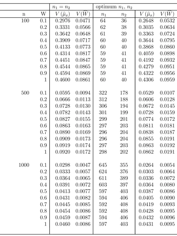
Table 4.1 below shows a comparison of variancesV ar(μbx) andV ar(Wc) when
using equal sample sizes and optimal sample sizes. Note that V ar(μbx) decreases
quite a bit whenn1 andn2 are chosen optimally as compared to equal sample sizes, but V ar(Wc) goes up slightly.
Table 4.1: Comparison of V (μbx) and V(Wc) for equal and optimal sample
sizes (optimized to minimize {V (μbx) +V(Wc)}) for μx = 4,σx2 = 4,
θ1 = 2, σS21 = 2, θ2 = 5,σS22 = 5, T =.3 n1 =n2 optimum n1, n2 n W V (μbx) V(Wc) n1 n2 V (μbx) V(Wc) 100 0.1 0.2976 0.0471 64 36 0.2648 0.0532 0.2 0.3331 0.0566 62 38 0.3035 0.0634 0.3 0.3642 0.0648 61 39 0.3363 0.0724 0.4 0.3909 0.0717 60 40 0.3644 0.0795 0.5 0.4133 0.0773 60 40 0.3868 0.0860 0.6 0.4314 0.0817 59 41 0.4059 0.0898 0.7 0.4451 0.0847 59 41 0.4192 0.0932 0.8 0.4544 0.0865 59 41 0.4279 0.0951 0.9 0.4594 0.0869 59 41 0.4322 0.0956 1 0.4600 0.0861 60 40 0.4306 0.0959 500 0.1 0.0595 0.0094 322 178 0.0529 0.0107 0.2 0.0666 0.0113 312 188 0.0606 0.0128 0.3 0.0728 0.0130 306 194 0.0672 0.0145 0.4 0.0782 0.0143 301 199 0.0728 0.0159 0.5 0.0827 0.0155 299 201 0.0774 0.0172 0.6 0.0863 0.0163 297 203 0.0811 0.0181 0.7 0.0890 0.0169 296 204 0.0838 0.0187 0.8 0.0909 0.0173 296 204 0.0855 0.0191 0.9 0.0919 0.0174 297 203 0.0863 0.0192 1 0.0920 0.0172 298 202 0.0862 0.0191 1000 0.1 0.0298 0.0047 645 355 0.0264 0.0054 0.2 0.0333 0.0057 624 376 0.0303 0.0064 0.3 0.0364 0.0065 611 389 0.0336 0.0072 0.4 0.0391 0.0072 603 397 0.0364 0.0080 0.5 0.0413 0.0077 597 403 0.0387 0.0086 0.6 0.0431 0.0082 594 406 0.0405 0.0090 0.7 0.0445 0.0085 592 408 0.0419 0.0093 0.8 0.0454 0.0086 592 408 0.0428 0.0095 0.9 0.0459 0.0087 594 406 0.0432 0.0096 1 0.0460 0.0086 597 403 0.0431 0.0095
CHAPTER V
SIMULATION STUDY AND CONCLUSIONS
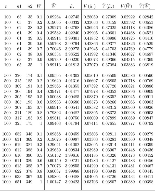
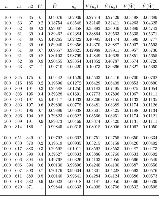
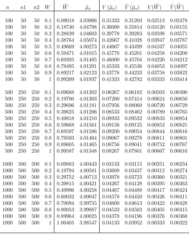
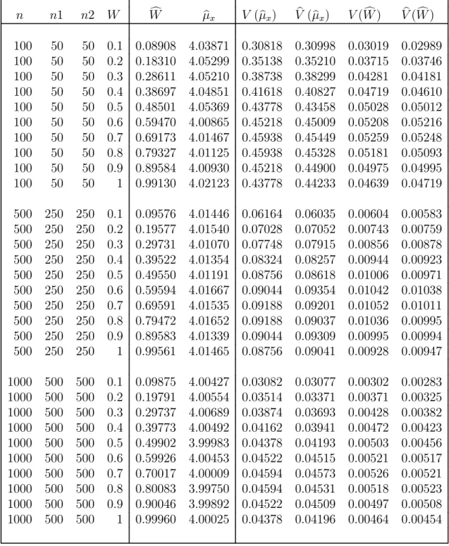
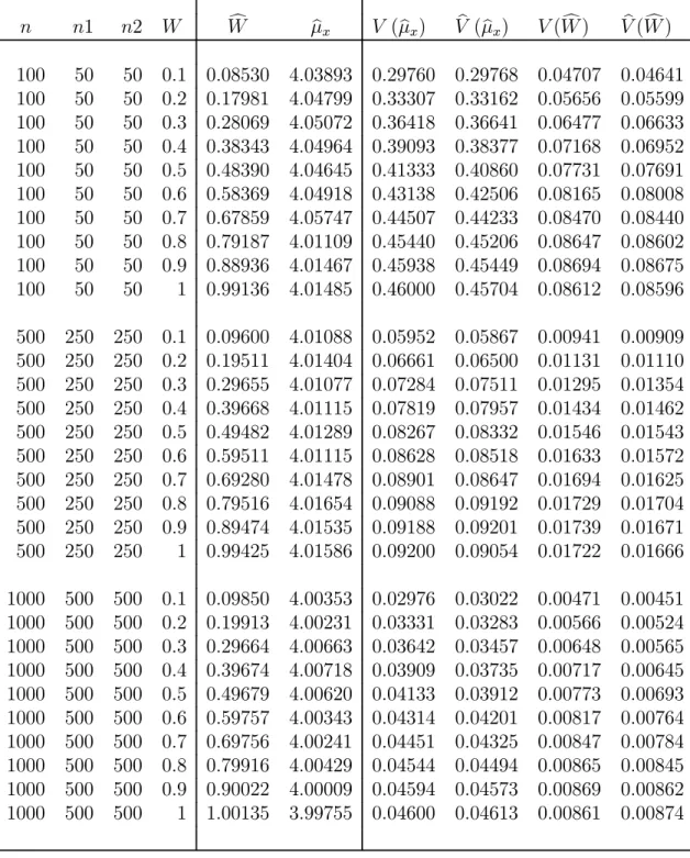
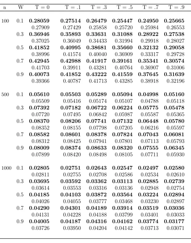
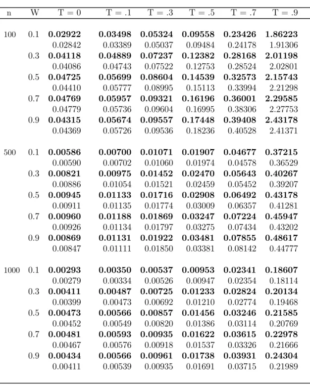
In this chapter we present results of a simulation study and provide some concluding remarks. The simulations are carried out using SAS (Windows version 9.1). The SAS code is provided in Section 5.4 of this chapter. For all simulations, the sensitive variable X is chosen to be a Poisson variable with mean μx = 4.
Although one could use any distribution for the simulations, we have chosen the Poisson distribution because it has been used in other comparable studies, and also it is a reasonable distribution when dealing with rare behaviors, in the sense that not everyone engages in these behaviors. The scrambling variables are also chosen to be Poisson for similar reasons: comparability with other studies and agreement with the parent distribution of the sensitive variable X. The scrambling variables S1 and S2 are specified to have means θ1 = 2 and θ2 = 5, respectively. These particular values for the means have been used in previous studies, thus allowing for reasonable comparison of our proposed model with earlier models. The results are averaged over 1000 simulation runs each with a sample size ofn= 100, n= 500, and n = 1000. Simulations using optimal sample sizes and equal sample sizes (n1 = n2) were run, as appropriate. The goals of these simulations are threefold. We want to verify that our simulated estimates agree with the correct values for μx
and W. Similarly, we want to make sure that the simulated variances are also in agreement with our theoretical variances. Finally, we want to verify that as values of n,T, and/or W change, expected trends can be seen in simulated results.
5.1 Quantitative Additive Optional RRT Models with Optimal Sample Selection
We would like to point out that the partial RRT models generally have the smallest variance and the optional models (both one-stage and two-stage) have much higher values forV ar(μbx). However, one should keep in mind that the partial RRT models
estimate only one parameter (μx), while the optional RRT models also estimate the
sensitivity level (W). Hence, comparing a partial RRT model to an optional RRT model would be unreasonable. So our simulation study will focus on how well a two-st