UCLA
UCLA Electronic Theses and Dissertations
Title Explaining Classifiers Permalink https://escholarship.org/uc/item/6bh039q5 Author Shih, Boyun Publication Date 2019 Peer reviewed|Thesis/dissertationUNIVERSITY OF CALIFORNIA Los Angeles
Explaining Classifiers
A thesis submitted in partial satisfaction of the requirements for the degree Master of Science in Computer Science
by
Boyun Shih
c
Copyright by Boyun Shih
ABSTRACT OF THE THESIS Explaining Classifiers
by Boyun Shih
Master of Science in Computer Science University of California, Los Angeles, 2019
Professor Adnan Youssef Darwiche, Chair
We study the task of explaining machine learning classifiers. We explore a symbolic approach to this task, by first compiling the decision function of a classifier into a tractable decision diagram, and thenexplaining its behavior using exact reasoning techniques on the tractable form. On the compilation front, we propose new algorithms for encoding the decision func-tions of Bayesian Network Classifiers and Binarized Neural Network Classifiers into tractable decision diagrams. On the explanation front, we examine techniques for generating a variety of instance-based and classifier-based explanations on tractable decision diagrams. Finally, we evaluate our approach on real-world and synthetic classifiers. Using our algorithms, we can efficiently produce exact explanations that deepen our understanding of these classifiers.
The thesis of Boyun Shih is approved.
Eliezer M Gafni Alexandr Sherstov
Adnan Youssef Darwiche, Committee Chair
University of California, Los Angeles 2019
TABLE OF CONTENTS
1 Introduction . . . 1
2 Background . . . 3
2.1 Tractable Decision Diagrams . . . 4
2.1.1 Ordered Binary Decision Diagrams . . . 4
2.1.2 Sentential Decision Diagrams . . . 5
2.2 Machine Learning Classifiers . . . 5
2.2.1 Bayesian Network Classifiers . . . 5
2.2.2 Naive Bayes Classifiers . . . 7
2.2.3 Binarized Neural Network Classifiers . . . 7
3 Compilation Algorithms . . . 8
3.1 Compiling Naive Bayes Classifiers . . . 8
3.2 Compiling Bayesian Network Classifiers . . . 9
3.3 Compiling Neural Network Classifiers . . . 19
3.A Proofs . . . 26 4 Explanation Techniques . . . 29 4.1 Instance-Based Techniques . . . 29 4.1.1 Prime Implicant . . . 29 4.1.2 Robustness . . . 30 4.1.3 Minimum Cardinality . . . 32 4.2 Classifier-Based Techniques . . . 32 4.2.1 Monotonicity . . . 33
4.2.2 Irrelevant Variables . . . 34
5 Experiments and Case Studies . . . 35
5.1 Bayesian Network Classifier Experiments . . . 35
5.2 Bayesian Network Classifier Case Study . . . 37
5.3 Binarized Neural Network Experiments . . . 39
5.4 Binarized Neural Network Case Study . . . 41
6 Conclusion . . . 45
LIST OF FIGURES
2.1 An OBDD represented using the diagram notation. . . 4 2.2 The DAG and CPTs of a Bayesian Network classifier. . . 6
3.1 Variable H splits feature variables into (U,V). When given an instantiation u
on the feature variables U, we can construct a subclassifier that has the same decision function as the original classifier over feature variables V. . . 10 3.2 Visualization of the equivalence interval of a classifier B. The red dots represent
instances classified as 1 and the blue dots represent instances classified as 0. A classifier that is similar toBshares the same decision function asBif its coefficient γ falls within the equivalence interval ofB, depicted by the white region between α and β. . . 13 3.3 Examples of classifier families with improved compilation time. . . 18 3.4 Learning the finite automaton for the 3 mod 4 counter. Using the counterexample
1101, we modify the hypothesis DFA into the updated DFA. . . 23
5.1 Three 16×16 images: digit 0, digit 8, and a smile. For each image we compile around its r-neighborhood (the used 8×8 images are not shown). . . 40 5.2 Prime implicant results for r = 6 for the images in Figure 5.1a and 5.1b. The
grey striped region represents ‘don’t care’ pixels. If we fix the black/white pixels in Figure 5.2a, any completing image within a radius of 6 from Figure 5.1a must be classified as ‘0’. If we fix the black/white pixels in Figure 5.2b, any completing image within a radius of 6 from Figure 5.1b must be classified as ‘8’. . . 42
5.3 Prime implicant results for r = 5 for the images shown in Figure 5.1. The grey striped region represents ‘don’t care’ pixels. If we fix the black/white pixels in Figure 5.3a, any completing image within a radius of 5 from Figure 5.1a must be classified as ‘0’. If we fix the black/white pixels in Figure 5.3b, any completing image within a radius of 5 from Figure 5.1b must be classified as ‘8’. If we fix the black/white pixels in Figure 5.3c, any completing image within a radius of 5 from Figure 5.1c must be classified as ‘8’. . . 43
LIST OF TABLES
2.1 The function on the 16 possible inputs computed by the OBDD in Figure 2.1b. The Bayesian Network classifier in Figure 2.2 also computes the same function. 6
5.1 win95pts has 76 nodes, 16 feature variables and width 9. Andes has 223 nodes, 24 feature variables and width 18. cpcs54 has 54 nodes, 13 feature variables and width 14. Width refers to the network tree-width, approximated by the minfill heuristic. . . 36 5.2 Network tcc4ehas 98 nodes and width 10. Network emdec6g has 168 nodes and
width 7. We use t27 as the class node for tcc4e, and x29 as the class node for emdec6g. . . 37 5.3 Compilation experiments . . . 44
ACKNOWLEDGMENTS
I would like to thank Adnan and Arthur for introducing me to the wonderful world of research. Thank you for being patient with me and providing me with a safe environment to explore my ideas and grow as a researcher.
I am grateful to have shared the lab space with the Automated Reasoning and the StarAI group. You guys never fail to keep up a lively and fun atmosphere in the lab. I will especially miss our many dining hall treks up the Hill.
I would also like to thank my family for being supportive of my goals, and always asking me to explain my research to you. Even when I’m unsuccessful, it pushes me to understand my own work more deeply.
CHAPTER 1
Introduction
Recent progress in artificial intelligence and the increased deployment of AI systems have led to the need forexplaining the decisions made by such systems, particularly classifiers [RSG16, EDF17, LL17, RSG18]. It is now recognized that opacity, or lack of explainability, is one of “the biggest obstacle[s] to widespread adoption of artificial intelligence” [CN17]. For example, one may want to explain why a classifier turned down a loan application, rejected an applicant for an academic program, or recommended surgery for a patient. Answering suchwhy? questions is important for gaining a user’s trust in the classification decision and for government regulations, such as the EU General Data Protection Regulation [GF17].
In this thesis, we propose a symbolic approach to explaining classifiers, which is based on the following observation [CD03]. Consider a classifier that labels instances either positively or negatively based on a number of binary feature variables. The classifier specifies a func-tion that maps features into a 0/1 decision (1 for a positive instance). We call this funcfunc-tion the classifier’s decision function, which unambiguously describes the classifier’s behavior, regardless of its implementation. Our goal is then to obtain a symbolic and tractable repre-sentation of this decision function, to enable efficient reasoning about its behavior, including generating explanations for its decisions. We refer to the constructing of the symbolic and tractable representation of a classifier’s decision function ascompiling the classifier.
Choosing the target representation of the decision function involves a trade-off between compilation cost and tractability of explanations. On one extreme, we can maintain the clas-sifier’s representation, incurring no compilation cost but possibly leaving many explanation tasks expensive. Another choice may be to compile the classifier into Conjunctive Normal Form (CNF) and answer explanation tasks using a SAT solver [NKR18]. In this thesis we
focus on compiling classifiers into Ordered Binary Decision Diagrams (OBDDs) [Bry86], which require a possibly costly compilation phase but enable us to answer many interesting explanation tasks in linear/quadratic time on the size of the decision diagram.
In particular, we study Naive Bayes, Bayesian Network, and Binarized Neural Network classifiers. We review an existing technique for compiling Naive Bayes classifiers into OB-DDs [CD03], and introduce new algorithms for compiling Bayesian Network and Binarized Neural Network classifiers into OBDDs. We then convert the OBDDs into Sentential De-cision Diagrams (SDDs) [Dar11], which can be much more succinct yet still maintain the tractability properties required for our explanation tasks.
Once we have the classifiers represented as tractable decision diagrams, we explore which explanation tasks are efficient on the decision diagrams. The explanation tasks we consider come in two flavors: instance-based or classifier-based. Instance-based explanations reason about the classifier’s behavior on one specific instance, and asks questions such as “What is the minimum perturbation required on this instance to flip its classification decision?” or “What is the minimal subset of features on this instance that can guarantee its classification decision, regardless of how the remaining features are flipped?” Classifier-based explanations reason about the classifier’s global behavior, and asks questions such as “Is the classifier monotonic?” Reasoning about these questions gives us insight into the behavior of the decision diagrams, which is exactly the behavior of the original classifiers.
We next provide an overview for the remaining chapters of this thesis. In Chapter 2, we define our notation and review material on tractable decision diagrams and machine learning classifiers. In Chapter 3, we describe an existing algorithm for compiling Naive Bayes classifiers and present novel algorithms for compiling Bayesian Network and Binarized Neural Network classifiers into OBDDs. In Chapter 4, we formally define our explanation tasks of interest and provide efficient algorithms for answering these tasks on our decision diagrams. Finally, in Chapter 5, we present experimental results and case studies, and conclude in Chapter 6.
CHAPTER 2
Background
We introduce notations and definitions, and review the relevant technical preliminaries. Capital lettersX denote variables and lower-case lettersxdenote their values, also called aliteral. Bold capital lettersX denote sets of variables and bold lower-case lettersxdenote their instantiations, also called an instance. When referring to machine learning classifiers, feature variables are the inputs andclass variable is the output of the classifier.
We begin with knowledge compilation, which examines languages for representing Boolean functions [CD97, DM02, SK96]. The languages that have been studied are generally subsets of Negation Normal Form (NNF). A NNF is a rooted, directed acyclic graph where each internal node is labelled with ∧ or ∨ and each leaf node is labelled with >, ⊥, or a literal. Note that negations (¬) can only appear with a literal, and not as an internal node.
A well-known subset of NNF is Conjunctive Normal Form (CNF). A CNF is a conjunction of clauses, where each clause is a disjunction of literals. This is also the subset of NNFs with height at most 2, where the children of each∨-node are leaves and the root is a ∧-node.
CNF is considered a representation language, since it is suitable for human specification and interpretation. But, it is not a target compilation language since there is no known efficient algorithm for important queries/transformations, such as model counting or nega-tion. These queries/transformations are necessary for generating explanations and reasoning about a Boolean function. As such, we next examine two target compilation languages that do efficiently support many queries/transformations.
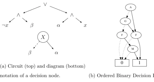
∨ ∧ ¬x β ∧ α x X β α
(a) Circuit (top) and diagram (bottom) notation of a decision node.
0 1 A F G F M
(b) Ordered Binary Decision Diagram
Figure 2.1: An OBDD represented using the diagram notation.
2.1
Tractable Decision Diagrams
The main properties that will give us tractability on many queries/transformations isdecision and ordering. A decision node is recursively defined as either >, ⊥, or a ∨-node with the form (X∧α)∨(¬X∧β), where α and β are decision nodes andX is a variable. In the last case, we say that the decision node is labelled byX. Binary Decision Diagram (BDD) is the subset of NNF where the root is a decision node.
2.1.1 Ordered Binary Decision Diagrams
An Ordered Binary Decision Diagram (OBDD) is a BDD that respects the ordering prop-erty [Bry86]. This means that the decision nodes of the OBDD respect some global ordering of the variables: if a decision node labelled by Xi is a parent of a decision node labelled by Xj, then Xi must come before Xj in the global ordering. Figure 2.1b shows the decision diagram notation of an OBDD with the variable orderingA, G, F, M, and sinks 0/1 denoting ⊥/>. To evaluate the OBDD on an instance x, start at the root and repeatedly follow the solid edge if the variable of the current node is set to 1 by x, and follow the dashed edge otherwise. The sink node that is reached determines the evaluation of x.
2.1.2 Sentential Decision Diagrams
A Sentential Decision Diagram(SDD) is a variation of the OBDD where the decision nodes decompose on sets of variables instead of single variables [Dar11]. A decision node labeled by variableXin an OBDD decomposes a function f into (¬X∧h0)∨(X∧h1). On the other
hand, a decision node in an SDD is labeled by a splitting of the variables into two sets X
and Y, and decomposes a functionf into (g0∧h0)∨. . .∨(gn∧hn), wheregi :X → {⊥,>}, hi :Y → {⊥,>}, andg1, . . . , gnare exhaustive and mutually exclusive. SDDs are a superset of OBDDs, since OBDDs can be seen as the special case when X (in the X,Y split of an SDD node) is a set with a single variable. For a more detailed treatment of SDDs, see [Dar11]. SDDs support almost all of the tractable operations that are offered by OBDDs [Dar11], and can be more succinct than OBDDs [Bov16]. There is also a comprehensive SDD software package with all of the necessary operations for running our explanation techniques [CD18].
2.2
Machine Learning Classifiers
We will now describe some commonly used machine learning classifiers. We consider versions of these classifiers that have binary inputs and outputs, so we can aim to compile their decision functions into tractable decision diagrams for reasoning and generating explanations.
2.2.1 Bayesian Network Classifiers
A Bayesian Network is a directed acyclic graph (DAG) along with conditional probability tables (CPTs) [Dar09]. In the DAG, nodes specify variables and edges specify conditional dependencies. A CPT specifies the distribution on a node for each state of its parents in the DAG. Together, the DAG and CPTs generate a probability distribution P r(.) over the variables of the Bayesian Network.
TheBayesian Network classifierswe consider are Bayesian Networks with a single binary class variableC,nbinary feature variablesX ={X1, . . . , Xn}, and a classification threshold t [FGG97]. The class C is a root in the network and the features X are leaves. A Bayesian
Network classifier classifies an instancex as 1 if P r(c|x)≥t and 0 otherwise, where P r(.) is the probability distribution specified by the underlying Bayesian Network. An example of a Bayesian Network classifier is shown in Figure 2.2, whose decision function matches the OBDD in Figure 2.1b. We provide the truth table in Table 2.1.
C
A
N1
G F M
N2
(a) Directed acyclic graph
Threshold 0.5 C= 1 0.5 C 0 1 A= 1 0.6 0.7 C 0 1 N1 = 1 0.3 0.9 N1 0 1 N2 = 1 0.3 0.7 N1 0 1 G= 1 0.5 0.6 N2 0 1 M = 1 0.2 0.9 N1, N2 00 01 10 11 F = 1 0.1 0.8 0.3 0.9
(b) Conditional probability tables and threshold
Figure 2.2: The DAG and CPTs of a Bayesian Network classifier.
Table 2.1: The function on the 16 possible inputs computed by the OBDD in Figure 2.1b. The Bayesian Network classifier in Figure 2.2 also computes the same function.
AGF M f(x) 0 0000 0 1 0001 0 2 0010 0 3 0011 1 AGF M f(x) 4 0100 0 5 0101 0 6 0110 1 7 0111 1 AGF M f(x) 8 1000 0 9 1001 0 10 1010 1 11 1011 1 AGF M f(x) 12 1100 0 13 1101 0 14 1110 1 15 1111 1
2.2.2 Naive Bayes Classifiers
A Naive Bayes classifier is a special type of a Bayesian Network classifier where there is an edge from the node of the class variable to the nodes of each feature variable, and there are no other edges or nodes.
2.2.3 Binarized Neural Network Classifiers
A Binarized Neural Network classifier is a feed-forward neural network where the weights and activations are binarized using {−1,1} [HCS16]. A Binarized Neural Network classifier is composed of internal blocks and one output block. Internal blocks consist of three layers: a linear transformation (LIN), batch normalization (BN), and binarization (BIN).
• The LIN layer has parameters a (weights) and b (bias). Given an input x, this layer returnsha,xi+b.
• The BN layer has parameters µ (mean), σ (standard deviation), α (weight), and γ (bias). Given an input y, this layer returns α(y−σµ) +γ.
• The BIN layer returns the sign (1 or −1) of its input.
The output block consists of a LIN layer and an ARGMAX layer. The ARGMAX layer picks the output class with the highest activation. More details regarding these blocks and layers and their exact definitions is given by Narodytska et al. [NKR18]. For convenience we consider a Binarized Neural Network classifier with outputs 0/1 instead of −1/1.
Both the Bayesian Network and Binarized Neural Network classifiers we consider have underlying decision functions that map binary inputs into a binary output. As such, we aim to compile their decision functions into tractable decision diagrams for efficient generation of explanations.
CHAPTER 3
Compilation Algorithms
In this section we explore techniques for compiling machine learning classifiers into tractable decision diagrams. The goal is to construct an OBDD that completely captures the decision function, or the input/output behavior, of the classifier.
We begin by reviewing an algorithm for compiling Naive Bayes classifiers from [CD03]. Then, we will introduce methods for compiling Bayesian Network and Binarized Neural Network classifiers, based on work published in [SCD19, SDC19].
3.1
Compiling Naive Bayes Classifiers
[CD03] proposed an algorithm for compiling a Naive Bayes classifier into an OBDD, while guaranteeing an upper bound on the time of compilation and the size of the resulting OBDD. In particular, for a classifier with n feature variables, the compiled OBDD has a number of nodes that is bounded by O(2n/2) and can be obtained in time O(n2n/2). Experimentally,
the time and space costs can still be quite low, depending on the classifier’s parameters and variable order used for the OBDD.
The algorithm is based on the following insights. Let X be all feature variables. Clas-sifying an instance x is based on the test P r(c|x)≥ t, which is equivalent to the following test [CD03].
P r(c)P r(x|c) P r(¬c)P r(x|¬c) ≥
t
1−t (3.1)
Since all the feature variables are independent in a Naive Bayes classifier, we can partition
s(u) = P rP r((uu|¬|cc)) and s(v) = P rP r((vv|¬|cc)). P r(c) P r(¬c) P r(u|c) P r(u|¬c) P r(v|c) P r(v|¬c) ≥ T 1−T (3.2) P r(c) P r(¬c)s(u)s(v)≥ t 1−t (3.3)
This formulation will help the efficient construction of OBDDs. In particular, at level k in our OBDD, we have 2k possible partial instantiations, leading to 2k values in {s(u) :
u∈ {0,1}|U|}. Moreover, there are onlyn−k remaining feature variables, leading two 2n−k values in {s(v) :v ∈ {0,1}|V|}. As such, we can bound the number of distinct subfunctions
at level k by O(min(2n,2n−k)), which gives us the same Sieling and Wegener bound on the number of OBDD nodes [Weg00]. To finish, the total number of nodes in the OBDD has a bound of 2Pn/2
k=1c2
k =O(2n/2) [CD03].
3.2
Compiling Bayesian Network Classifiers
We now present the algorithm for compiling Bayesian Network classifiers, which is more involved since the feature variables of the classifier are not necessarily independent. As such, we cannot partition the feature variables X in any way, since those inU may interact with those inV in the Bayesian Network.
Our compilation algorithm is based on recursively decomposing into smaller classifiers and identifying those that are equivalent to avoid the compilation of a classifier if an equivalent one has already been compiled. We first describe the method of decomposing into smaller classifiers, which can be described at a high level as follows. Given a Bayesian Network classifier B, let U and V be a partition of its features variables X and let H be a variable not inX. Suppose now that we are only interested in classifying instancesxthat set feature variablesU to some stateu. When certain conditions hold, we can perform the classification using a smallerclassifier, which is obtained from classifier B as follows:
– Node H is disconnected from its parents and C, the class node, is added as the new parent of H.
H U V C (a) ClassifierB. V C H (b) Subclassifier BHu.
Figure 3.1: Variable H splits feature variables into (U,V). When given an instantiation
u on the feature variables U, we can construct a subclassifier that has the same decision function as the original classifier over feature variables V.
– A CPT is assigned to H based on inference on B. – A prior is assigned to C based on inference on B.
– Leaves are repeatedly removed from classifier B as long as they are not inC∪H∪V. The resulting classifier is called asubclassifier. Figure 3.1 depicts an example of the structural changes needed to construct a subclassifier. We let FB denote the decision function of the original classifier B and FBH
u denote the decision function of the subclassifier B
H
u. The main
insight regarding these subclassifiers is that for any u and its corresponding subclassifier, FBH
u(v) = FB(uv) for any v. This key property will be used in the algorithm to reduce the
compilation of a classifier into the compilation of subclassifiers.
We will now spell out the above result on subclassifiers. We first state the conditions under which a subclassifier can be constructed.
Definition 1 Let (U,V) be a partition of the feature variables X in a Bayesian Network classifier B, and let H be a variable outside X. We say that H splits feature variables X
into (U,V) if H d-separates feature variables V from C and U.
Definition 2 Let B be a Bayesian Network classifier, H be a variable that splits feature variables into (U,V), and u be an instantiation of feature variables U. The subclassifier
for H and u, denoted BH
u, is obtained from classifier B as follows:
1. Disconnect node H from its parents.
2. Make H a child of class variable C, and set its Conditional Probability Table (CPT) to P(H|Cu).
3. Set the CPT of C to P(C|u).
4. Repeatedly remove every leaf node from B that is not in C∪H∪V.
Constructing a subclassifier requires some computational work on the original classifier B. First, we need to identify a variable H that satisfies the condition of Definition 1. This can be done in polynomial time as it only involves reasoning about d-separation [Dar09]. Second, we need to determine the CPTs of H and C, which require the computation of posteriors on the H and C, given the state u of feature variables U. This requires exact inference on the classifier B. We will later provide a bound on the number of inference calls made by our compilation algorithm for this purpose. The next theorem formalizes the property of subclassifiers.
Theorem 1 Let B be a Bayesian Network classifier and let H be a variable that splits feature variables into (U,V). For a subclassifier BH
u, we have FB(uv) = FBH
u(v) for all
instantiations v of feature variables V.
According to this theorem, the classification of an instance uv by classifier B will match the classification of v by subclassifier BH
u. As we shall see, when our compilation algorithm
fixes the state of feature variables U to u, it will construct and recursively compile the subclassifierBH
u.
We will now introduce the second key result that will form the basis of our algorithm for compiling a Bayesian Network classifier into an OBDD. This result provides a method for detecting when two “similar” Bayesian Network classifiers induce the same decision function.
In this section we assume, without loss of generality, that the classifier has a class node C which has a single child H. This assumption is satisfied by all subclassifiers and can easily be satisfied for any classifier by adding a dummy class node with the original class node as its single child. First we define when two classifiers are considered similar.
Definition 3 LetB be a Bayesian Network classifier with a class node C which has a single child node H. A second Bayesian Network classifier is similar to B if it has the same structure as B and differs only in the CPTs of C and H.
Let X be the feature variables of two similar classifiers B and B0. Note that P(X|H) is the same across the two classifiers, and H d-separatesC fromX by our earlier assumption. Thus, we can rewrite P(C|X) as follows:
P(C|x) =X h P(C|h)P(h|x) =X h P(C, h)P(x|h)/P(x) (3.4)
So far, these results have not assumed that the class variable C and the variable H are binary. For the rest of this section, we will assume that nodesC and H are binary, and the classification threshold is t. In this setting, we have an efficient way of detecting when two similar classifiers share the same decision function, in time linear in the number of feature variables X. We present the details next.
Setting ah = P(c, H = h)−tP(H = h), we can rewrite the classification as a linear inequality. X h P(c, h)P(x|h)≥tP(x) X h (P(c, h)−tP(h))P(x|h)≥0 X h ahP(x|h)≥0 (3.5)
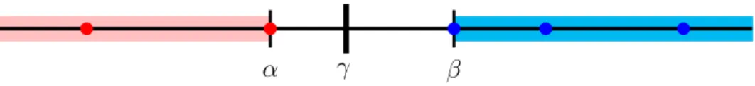
α γ β
Figure 3.2: Visualization of the equivalence interval of a classifier B. The red dots represent instances classified as 1 and the blue dots represent instances classified as 0. A classifier that is similar toB shares the same decision function asB if its coefficientγ falls within the equivalence interval of B, depicted by the white region between α and β.
of values ah classify all instancesx the same way. To do so, we define the sign, margin, and coefficient of such classifiers.
Definition 4 Let B be a non-trivial1 Bayesian Network classifier with a threshold t and a
binary class node C which has a single binary child node H. Let σ denote the sign of the classifier, which is defined to be 1 if P(c|H = 1)≥t and 0 otherwise. The marginα, β and
coefficient γ of B are defined as follows:
α = max x:FB(x)=1P(x|H = 1−σ)/P(x|H =σ) β = min x:FB(x)=0P(x|H = 1−σ)/P(x|H =σ) γ = −1· P(c, H =σ)−tP(H =σ) P(c, H = 1−σ)−tP(H = 1−σ)
That is, α is the largest value of P(x|H = 1−σ)/P(x|H = σ) attained by any instance classified as 1, and β is the smallest such value attained by any instance classified as 0 (see Figure 3.2). The values α, β, and γ come from a rearrangement of Equation 3.5 for the case of a binary H variable. The notion of a margin was actually identified by [CD03] in connection to Naive Bayes classifiers, and turns out to apply to general Bayesian Network classifiers.
The next result was proven only for Naive Bayes classifiers in [CD03]. We generalize this to Bayesian Network classifiers.
1A non-trivial classifier with a binary class node classifies at least one instance as 1 and at least one
Theorem 2 Let B be a non-trivial Bayesian Network classifier with a binary class node C and a single binary child node H. Let B0 be a second classifier that is similar to B and has the same sign as B. Let t be their threshold, (α, β) be the margin of classifier B, and γ be the coefficient of B0. The two classifiers have the same decision function, FB = FB0, iff γ belongs to the interval [α, β). This is called the equivalence interval of classifier B.
The above theorem enables us to perform binary search over equivalence intervals to identify equivalent subclassifiers: ones that lead to the same decision function and hence the same compilation. This technique avoids the compilation of a subclassifier if an equivalent one has already been compiled.
From Bayesian Network Classifiers to OBDDs
We now present the full algorithm for compiling a Bayesian Network classifier B into an OBDD. We first identify a binary variable H that splits the feature variables into (U,V). We then start enumerating over the values of feature variables in U as if we are building a decision tree, in a depth-first manner. Each leaf of this decision tree corresponds to a distinct instantiation uand a subclassifier BH
u with its equivalence interval. These subclassifiers are
similar to one another, since they differ only in the CPTs of class C and variable H. Our algorithm will then compile these subclassifiers recursively using the same technique, except that it will avoid compiling a subclassifier if it already compiled an equivalent one—as determined by Theorem 2.
The efficiency of this algorithm depends on the choice of variable H and the correspond-ing feature variable decomposition (U,V), as we want the size ofU to be small. We identify such feature variable decompositions in a preprocessing step. That is, after first decompos-ing feature variables into (U,V) using an appropriate H, we follow by decomposing V
recursively. This leads us to the notion of ablock ordering of feature variables.
Definition 5 Given a Bayesian Network classifier, ablock orderingof its feature variables
X, and for each 0< k < m, there exists a binary variable H that splits feature variables X
into (X1∪. . .∪Xk,Xk+1∪. . .∪Xm).
Each element Xi is called a block of the block ordering π. We will assume that the feature variables in a block are ordered (arbitrarily). As such, we will refer to feature variables by their position in the block ordering π.
We will later discuss a heuristic for obtaining a block order, which we used in our exper-iments. But for now, we will discuss Algorithms 1 and 2. Algorithm 1 is passed a Bayesian Network classifier B and a block orderingπ of feature variables. It creates the sinks of the OBDD and calls Algorithm 2.
Algorithm 2 implements the proposal we discussed earlier. It maintains a cache that stores tuples of the form (D, I, σ, k), whereDis an OBDD node, I is an equivalence interval, σ is a boolean, and k is an integer. Such a cache entry means that OBDDD is the result of compiling a subclassifier Bu that has equivalence interval I and sign σ. It also means that
the last feature variable in block U is at position k−1 in the block ordering π. The cache is fetched based on a coefficient γ, a sign σ and a level k. That is, it returns OBDD D if γ ∈I for the same σ and same k.
Algorithm 2 makes use of four auxiliary functions. First,get-subclassifier(B,u, π, k) constructs a subclassifier and requires a constant number of calls to an exact inference algorithm to get the coefficients of the subclassifier. get-sink(B) takes in a subclassifier with no more feature variables, and returns either the 0-sink or the 1-sink based on a simple check. equivalence-interval(D) computes the equivalence interval of the classifier leading to OBDD D. This is done in constant time using the equivalence intervals for the children of D [CD03]. Finally, get-OBDD-node(S) returns an OBDD node, which is defined by the set S that specifies the node’s children and the labels of edges pointing to these children.
Algorithm 1 compile-classifier(B, π)
input: Bayesian Network classifier B and block orderingπ of feature variables
output: OBDD for the decision function of classifierB
main:
1: 0-sink ←terminal OBDD node labeled with 0
2: 1-sink ←terminal OBDD node labeled with 1
3: D←compile-subclassifier(B,{}, π,0)
4: return reduced form ofD
Algorithm 2 compile-subclassifier(B,u, π, k)
input: Bayesian Network classifier B, instantiation u of some feature variables, block ordering π
of feature variables, integerk
output: OBDD for the decision function of classifierB
main:
1: if u is an instantiation of a block in orderingπ then
2: B ← get-subclassifier(B,u, π, k)
3: if B has no feature variables then
4: return get-sink(B)
5: γ, σ ←coefficient and sign of B 6: D←find-in-cache(γ, σ, k) 7: if D=null then 8: D←compile-subclassifier(B,{}, π, k) 9: I ←equivalence-interval(D) 10: store-in-cache(D, I, σ, k) 11: return D
12: X← feature variable at position kin ordering π 13: S← {}
14: foreach state x of feature variable X do
15: C ←compile-subclassifier(N,u∪x, π, k+ 1)
16: add (C, x) to set S 17: return get-OBDD-node(S)
Algorithm 3 implements a simple, greedy heuristic for obtaining a block ordering of feature variables. Its running time is O(n4), where n is the number of feature variables,
which was sufficient for our experiments. Algorithm 3 block-order(B,X)
input: A Bayesian Network classifier B with feature variablesX
output: A block orderingπ of the feature variables X
main:
1: H,U,V ← class variable ofB,X,∅
2: foreach variableH0 that splits feature variablesX into (U0,V0) do
3: if |U0| ≤ |U|then
4: H,U,V ←H0,U0,V0
5: u←some instantiation of U
6: return U,block-order(BHu,V)
We close this section by providing time and size bounds on our compilation algorithm. We later show that for certain classes of Bayesian Networks, these bounds can be as tight as the bounds provided by [CD03] for compiling Naive Bayes classifiers into OBDDs.
Definition 6 Letπ= (X1, . . . ,Xm)be a block ordering of the feature variables in a Bayesian Network classifier B. Let pi denote the number of feature variables in block i, and let s(i, j) = Pj
k=ipk. The width wπ of this order and the compilation width wB of clas-sifier B are defined as:
wπ = max i∈{1,...,m} pi·min(s(1, i−1), s(i, m) ] wB = min π wπ.
We now have the following bounds on Algorithm 1.
Theorem 3 The number of nodes in the OBDD returned by Algorithm 1 is O(2wπ), where wπ is the width of order π. Moreover, the running time of the algorithm is O(P T +wπ2wπ), where P is the sum of the state space sizes of blocks in π and T is the time of an inference call on the classifier.
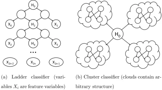
H0 H2 X0 X1 H4 X3 X2
...
X2n-2 X2n X2n-1(a) Ladder classifier (vari-ablesXiare feature variables)
H
0(b) Cluster classifier (clouds contain ar-bitrary structure)
Figure 3.3: Examples of classifier families with improved compilation time.
Consider the family of ladder classifiers depicted in Figure 3.3a, which has n = 2m+ 1 feature variables. We can use the sequence of nodes H2, H4, . . . , H2m to decompose feature variables, leading to the block ordering
[X0, X1],[X2, X3], . . . ,[X2m−2, X2m−1, X2m],
which has widthn/2. The size of the OBDD isO(2n/2) and the running time isO(nT+n2n/2).
The family of cluster classifiers in Figure 3.3b has similar bounds. Assume that we have n feature variables and k clusters, with each cluster having n/k feature variables. We can repeatedly use the node H0 to split feature variables into k blocks of size n/k, leading to a
block order width n/2, and a largest block size n/k. The size of the OBDD is O(2n/2) and
the running time is O(k2n/kT +n2n/2).
What is interesting about these bounds is that they match the ones for compiling Naive Bayes classifiers to OBDDs [CD03]—an NP-hard problem as shown by [SCD18b]. In practice, however, the time and space costs of Algorithm 1 can be quite low as we show in the experiments in Chapter 5.
3.3
Compiling Neural Network Classifiers
In this section, we explore the compilation of Binarized Neural Network classifiers (BNNs) into OBDDs. We have the same motivations as before, except this time we may be interested in only compiling the decision function over an input space, rather than over all possible inputs. For example, users of a BNN can pinpoint a particular input instance x and ask for guarantees on the behavior of the BNN for other inputs in the neighborhood of x. This has practical applications for image classification, where users expect an image of a dog to remain classified as a dog if only a few pixels are modified.
LetB be a BNN, and letBSrepresent the function ofB onS, an input region of interest. To obtain BS in a tractable form, we propose an Angluin-style algorithm for learning the OBDD representation of BS [Ang87]. Our algorithm leverages an existing technique for learning an OBDD using standard membership and equivalence queries [Nak05]. First, we construct a hypothesis OBDD and then iteratively call equivalence queries, adding OBDD nodes until its output agrees with BS. To answer equivalence queries efficiently, we encode the BNN and the hypothesis OBDD into a CNF, and require that the region S can be encoded as a CNF as well. When the algorithm terminates, it returns an OBDD D such thatD(x) =B(x) :∀x∈S, a notion related to theConstrainoperator on OBDDs [MT98]. We then verify properties of BNN B by performing efficient verification queries on OBDD D.
Our algorithm can also be used as an incremental and anytime compilation algorithm, by slowly increasing the region of interest. The compiled OBDD of a smaller region can be used as the hypothesis OBDD for the compilation task of a larger region, without starting over. We can essentially save our progress, and build on it at a later time if we decide the initial region is too small.
We next provide the encoding of BNNs and OBDDs into CNF, which will serve an important role in our main compilation algorithm.
BNN to CNF
We use the conversion given by Narodytska et al. [NKR18]. An internal block of a BNN consists of three layers: a linear transformation (LIN), batch normalization (BN), and bi-narization (BIN). The LIN layer has parameters a (weights) and b (bias). The BN layer has parameters µ (mean), σ (std), α (weight), and γ (bias). Put together, the three layers of an internal block can be translated to the following function h(x) on an input instance
x [NKR18].
h(x) = 1 ⇐⇒ ha,xi ≥ −σ
αγ+µ−b
Since the weightsaand input xare binarized as{−1,1}, the above computation reduces to a cardinality constraint of the form Pm
i=1li ≥ C, where li ∈ {0,1} and C ∈ R. This cardinality constraint can be encoded as a CNF.
The output block has a LIN layer followed by an ARGMAX layer, which can be encoded using a similar technique. First, we encode a cardinality constraint for all pairs of classes, which tells us the class that has a higher activation function in the pairing. Then, we use a final set of cardinality constraints to determine the class that was the winner in all of its pairings [NKR18]. Since we focus on Neural Networks with binary output classes in this paper, a single CNF variable is enough to represent the output of the BNN.
The space complexity of this conversion is O(N C2), where N is the number of neurons
in the BNN andC is the constant from the above cardinality constraint.
OBDD to CNF
We convert an OBDD into a CNF using the well-known Tseitin transformation [Tse68], which converts a Boolean circuit into a CNF. Consider an OBDD node labelled by variable X. If the two children of this node compute Boolean functionsC0, C1, then the OBDD node
computes the Boolean function R = (C0 ∧ ¬X)∨(C1 ∧X). We can then represent the
¬R∨C0∨X
¬R∨C1∨ ¬X
¬R∨C0∨C1
R∨ ¬C0∨X
R∨ ¬C1∨ ¬X
Applying this conversion to all OBDD nodes leads to a CNF representation of the Boolean function computed by the OBDD. The number of CNF clauses produced by this conversion is 5N, where N is the number of OBDD nodes.
The above encodings allow us to convert a BNN into a CNF αand an OBDD into a CNF β. Let X be the CNF variables corresponding to the BNN inputs and O be the variable corresponding to its output. Then α∧x∧O will be satisfiable iff the BNN outputs 1 under inputx. Similarly,α∧x∧ ¬O will be satisfiable iff the BNN outputs 0 under inputx. Now letX be the CNF variables corresponding to the OBDD variables andR be the variable we introduced for the OBDD root. Then β∧x∧R will be satisfiable iff the OBDD outputs 1 under input xand β∧x∧ ¬R will be satisfiable iff the OBDD outputs 0 under input x.
When the BNN and the OBDD share the same inputs x, we can check for their inequiv-alence with the formula φ =α∧β ∧(O∨R)∧(¬O ∨ ¬R) [NKR18]. Then, φ is satisfiable iff there is some instantiation of x such that (O ∧ ¬R)∨(¬O ∧R) (i.e. BNN and OBDD disagree).
Angluin-Style Exact Learning of Finite Automaton
In this section we describe Angluin’s algorithm for learning Deterministic Finite Automata (DFA) [Ang87]. The DFA learning algorithm has an adaptation for learning OBDDs [Nak05], which serves as the backbone for our neural network compilation algorithm. DFAs and OBDDs are initimately related: a Complete OBDD (an OBDD that does not skip vari-ables [Weg00]) is also a DFA (but a DFA is not necessarily an OBDD).
We roughly summarize the exposition on the topic of learning DFAs from the textbook by Kearns and Vazirani [KV94]. The learning algorithm falls under the category of active learning where the algorithm can learn through experimentation, as opposed to passive
learning where the algorithm has no control over the sample of examples. To learn the DFA for a function f, the learning process requires access to oracles for two types of queries:
• Membership Queries: The learning process selects an instancexand the oracle returns the value off(x).
• Equivalence Queries: The learner submits a hypothesis automaton h. The oracle tells the learner ifhcomputes the correct function (i.e. h=f), otherwise the oracle returns a counterexamplex for which h(x)6=f(x).
The main idea of the algorithm is as follows. Let S be the set of states of a minimal DFA we want to learn. Recall that each state represents a distinct equivalence class of input strings. At all times we keep a hypothesis DFA whose states S? represent a partition of S. We iteratively refine the partition by splitting some partition element of S? into two, so that |S?| increases. When|S?| =|S|, each element in the partition contains exactly one equivalence class from S, so our hypothesis DFA computes the target DFA.
Initially, we start with a one-node hypothesis DFA with just one state, which partitions all the states inS into one group. As long as our DFA is incorrect, we will receive counterex-amples from the equivalence query. Given a counterexample e, we can simulate e on our hypothesis DFA and identify the first states? for which its following step in the simulation is provably incorrect. This can be done efficiently by maintaining a binary classification tree, the details of which we omit. We then refine the partition by splitting s? into two nodes. This process repeats until we have learned all the states ofS, at which point the equivalence query gives no more counterexamples and our algorithm terminates.
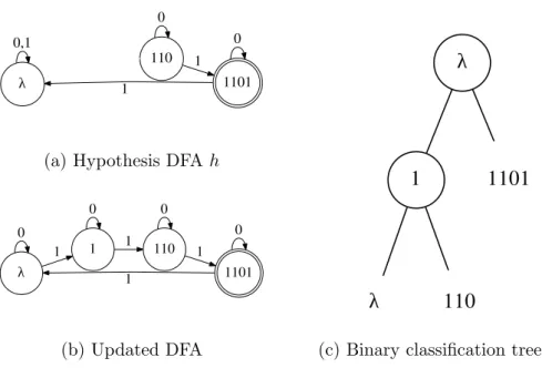
Suppose we wish to learn a DFA on binary inputs for the 3 mod 4 counter f, and we currently have the hypothesis DFA h in Figure 3.4a and its binary classification tree in Figure 3.4c. Since h(1101) = 0 6= f(1101), we get the string 1101 as a counterexample. Using the binary classification tree along with membership queries, the algorithm identifies the state λ in h as faulty, and splits it into two. This generates the updated DFA in Figure 3.4b, which computes f correctly.
λ 0,1 110 0 1101 1 1 0
(a) Hypothesis DFA h
λ 0 1 1 0 110 1 0 1101 1 1 0 (b) Updated DFA
λ
1
1101
λ
110
(c) Binary classification tree of h
Figure 3.4: Learning the finite automaton for the 3 mod 4 counter. Using the counterexample
1101, we modify the hypothesis DFA into the updated DFA.
The automaton learning algorithm was adapted into an OBDD learning algorithm by Nakamura [Nak05]. This variation requires n equivalence queries and 6n2+nlog(m) mem-bership queries, wheren is the number of nodes in the final OBDD andm is the number of variables in the OBDD.
BNN Compilation Algorithm
We now describe our main contribution: a compilation algorithm from a BNN to an OBDD. Given a BNN B onn binary inputs and one binary output, we wish to obtain an OBDD D that computes the function of B on a region S (i.e. D(x) = B(x) : ∀x ∈ S). We require region S to be encoded as a CNF.
Algorithm 4 implements our proposal. The subroutines BNNToCNF and OBDDToCNF per-form the encodings described earlier. We encode the BNN B as a CNF α with output variable O. Then, we start the OBDD learning algorithm as described in Section 3.3 to learn the reduced OBDD representation of B. The learning algorithm creates a hypothesis OBDDD, which we encode as a CNFβ with variableRrepresenting the OBDD output. We
Algorithm 4 CompileBNN(B,X, S)
input: A Binarized Neural Network B with input variables X, and a CNF S encoding an input region
output: An OBDDD computing the function of B on S main:
1: α, O←BNNToCNF(B,X) 2: D← initial hypothesis OBDD 3: β, R←OBDDToCNF(D,X)
4: φ←α∧β∧(O∨R)∧(¬O∨ ¬R)∧S 5: while φ has a satisfying assignment sdo 6: x← projection ofs onX
7: D←UpdateHypothesis(D,x) 8: β, R ←OBDDToCNF(D,X)
9: φ ←α∧β∧(O∨R)∧(¬O∨ ¬R)∧S 10: return D
setφ on Line 4 such thatφ has a satisfying assignment iff the current hypothesis OBDD D does not compute the same function as BNN B on region S. While φ is satisfiable, we take the satisfying assignment and keep only the variables corresponding to the BNN/OBDD in-puts as our counterexamplex. The subroutine UpdateHypothesisthen edits our hypothesis OBDD using counterexample x. Once we have an unsatisfiable φ, we return the OBDD D with the guarantee that it computes the same function as BNNB onS. Note that there are no guarantees on the output of OBDD D on instances outside S. The number of iterations of the while loop is N, where N is the number of nodes in the final outputD.
In Algorithm 5 we propose the construction of an input region that captures all instances in the neighborhood of some instancexonn variables. More specifically, Algorithm 5 takes in an instancex, a radius r, and outputs a CNF S on variables X1, . . . , Xn. An instancex? is a satisfying assignment for S iff the Hamming distance between x and x? is no greater than r. This becomes a cardinality constraint, which can be encoded in many ways [BB03].
Algorithm 5 r-RadiusDomain(x, r)
input: An input x=x1, . . . , xn and a radius r≤n
output: A CNF that encodes all instances x? such thath(x,x?)≤r, wherehmeasures the Hamming distance
main:
1: d← a 2D array with dimensions [0, n]×[0, r] 2: for j ←0 to r do 3: d0,j ← > 4: for i←1 to n do 5: for j ←0 to r do 6: h←di−1,j 7: l ←di−1,j−1 if j >0 else⊥
8: di,j ← OBDD node: label Xi, xi-child h,¬xi-child l 9: return OBDDToCNF(dn,r,X)
For ease of exposition, we use an OBDD for the constraint and then convert it to CNF. In the algorithm, node di,j stores the state with n −i variables processed and a current Hamming distance of r−j. On Line 8, the child edge of di,j that agrees with xi points to di−1,j. The other child edge points to di−1,j−1 if j >0, otherwise it points to⊥. By using S
as an input for Algorithm 4, we can compile an OBDD that exactly computes the function of a BNN for all instances close to some instance of interest, measured by the number of differing variables. The time and space complexity of Algorithm 5 isO(nr).
To extend our algorithm into an anytime compilation algorithm, we start with a small region of interest and increase its size over time. The compiled OBDD D will compute the same function as B on this small region. To compile the OBDD for a larger region, we can feed in D as the initial hypothesis OBDD in Algorithm 4 on Line 2, without the need to build D from scratch. Then, we can use the updated OBDD to verify the properties of B on the enlarged region. We can continue to enlarge this region until it becomes {0,1}n, at which point S =>and the compiled OBDD computes the same function as B everywhere.
3.A
Proofs
Proof of Theorem 1 We want to show that FB(uv) = FBH
u (v). We let P(.) denote the
probability distribution of the original classifier B and let P0(.) denote the probability dis-tribution of the subclassifier BuH. First, we work out the following equalities:
P(h|u) =X c P(h|cu)P(c|u) =X c P0(h|c)P0(c) =P0(h) P(v|u) =X h P(v|hu)P(h|u) =X h P(v|h)P(h|u) =X h P0(v|h)P0(h) =P0(v)
This gives us the following list of identities:
P(c|u) =P0(c) P(h|cu) = P0(h|c) P(h|u) =P0(h) P(v|u) = P0(v)
Next, we will show the main property we are after: for any cand v, P(c|uv) =P0(c|v). P(c|uv) =X h P(c|huv)P(h|uv) =X h P(c|hu)P(h|vu) =X h P(h|cu)P(c|u) P(h|u) P(v|hu)P(h|u) P(v|u) =X h P0(h|c)P0(c) P0(h) P0(v|h)P0(h) P0(v) =X h P0(c|h)P0(h|v) =P0(c|v)
Proof of Theorem 2 We let P(.) denote the probability distribution of the classifier B and let P0(.) denote the probability distribution of the classifier B0. Using Equation 3.5 we can rewrite the classification decision of classifier B as P
hahP(x|h) ≥ 0, where ah = P(c, H =h)−tP(H =h). Sinceh is binary, we can expand the summation.
a0P(x|H = 0) +a1P(x|H = 1)≥0
Since the classifier B is nontrivial, we know that a0/a1 <0. Suppose that the sign σ of
B is 1, and thus a1 >0. Rearranging, we get:
−1· a1 a0
≥ P(x|H = 0)
P(x|H = 1) (3.6)
Now supposeFB(x) = 1 for somex. Recall thatαis the maximum value of P(x |H=0)
P(x|H=1) attained
by any instance classified as 1. Let a0h =P0(c, H =h)−tP0(H =h). −1· a 0 1 a0 0 =γ ≥α≥ P(x|H = 0) P(x|H = 1)
So we have that FB0(x) = 1. The proof is analogous for instances classified as 0, as well as for classifiers with sign 0, thus FB(x) =FB0 (x) for all x.
Proof of Theorem 3 Letπ = (X1, . . . , Xm) be the block ordering of the feature variables, and let s(i, j) = Pj
k=ipk, where pk denotes the number of feature variables in block k. Let tk be the number of OBDD nodes in levels s(1, k−1) to s(1, k)−1, so Pktk is the total number of nodes in the OBDD.
We will bound the number of nodes in the OBDD by bounding the number of nodes in each block. The number of OBDD nodes on level s(1, k−1) is bounded from above by 2s(1,k−1) (by decision trees) and also by 2·2s(k,m) (by equivalence intervals). The bound of
2·2s(k,m) from equivalence intervals is due to the following observation. For the subclassifiers
stored in cache of sign 1 and levels(1, k−1), their classification decision on an instancexcan be written as in Equation 3.6. Since the RHS of the inequality of Equation 3.6 is the same among all subclassifiers of sign 1 and levels(1, k−1), and there are 2s(k,m) distinct instances
1 and level s(1, k−1). The analysis for subclassifiers of sign 0 and level s(1, k−1) is the same, so we have at most 2·2s(k,m) equivalence classes for subclassifiers on levels(1, k−1).
From levels(1, k−1) to levels(1, k)−1, the algorithm constructs the OBDD in a decision tree manner. Therefore, we have that tk is bounded by pk· min(2s(1,k−1),2·2s(k,m)). So, tj = O(2wπ), where j = argmaxk(tk). To finish, observe that both sequences tj+1, tj+2, . . .
and tj−1, tj−2, . . . on either side of j decay exponentially fast, so we have that the total
number of nodes is P
ktk =O(tj) =O(2 wπ).
Next we will bound the time complexity of the algorithm. We start by showing that the number of exact inference calls is P =p1+. . .+pm. This number is much smaller than the number of subclassifiers constructed, which is O(2wπ), because we can share the results of inference calls across different subclassifier constructions.
We want to show that for multiple classifiers that are similar, the construction of their subclassifiers can reuse the same inference calls. For a set of similar classifiers, let H0 be the child of class nodeC and letH be the new splitting node used to construct the subclassifiers. Note that to construct a subclassifier, we need the values P(h|uc) and P(c|u).
P(h|uc) =X h0
P(h|uch0)P(h0|c)
The terms P(h|uch0) are actually the same across similar classifiers, since similar classi-fiers only differ in the CPTs of C and H0 and those variables are fixed in these terms. As well, the terms P(h0|c) do not require any inference at all, since these are just the CPTs encoded in the network. A similar analysis shows that inference calls can also be shared when calculating the value of P(c|u). Therefore, the total number of inference calls for the i-th block is O(pi). Finally, computing equivalence intervals in the algorithm can be done without any inference calls using the equivalence intervals of subclassifiers. So, the total number of inference calls is O(P).
As for the number of computations of the algorithm, observe that the most expensive operation is finding and storing equivalent subclassifiers in cache, which requires binary search on O(2wπ) intervals. This gives usO(w
CHAPTER 4
Explanation Techniques
In Chapter 3, we examined compilation algorithms for converting the decision function of machine learning classifiers into OBDDs. In this section, we will leverage the tractability of OBDDs to develop efficient methods for reasoning and generating explanations for these decision functions. OBDDs can handle a wide range of queries and transformations in polynomial time, which will serve as building blocks for our explanation techniques. The work in this chapter is published in [SCD18a, SCD18b]
We describe these explanation techniques with respect to a decision function, rather than a classifier, so the set of all variables in the explanations is the set of all feature variables in the original classifier. We first look at instance-based techniques, which analyze a decision function with respect to a particular instance. Then, we will contrast this with classifier-based techniques, which examine a decision function more generally, taking into account every possible input instance. We will then use these explanation techniques to analyze the behavior of machine learning classifiers in Chapter 5.
4.1
Instance-Based Techniques
4.1.1 Prime ImplicantThe first class of explanations we consider is prime-implicant, or PI for short. These expla-nations answer the following question: what is the smallest subset of variables that renders the remaining variables irrelevant to the current decision? In other words, which subset of variables—when fixed—would allow us to arbitrarily toggle the values of other variables, while maintaining the classifier’s decision?
Let y and z be instantiations of some variables and call them partial instances. We will write y ⊇ z to mean that y extends z. That is, it includes the variables in z but may set some additional variables.
Definition 7 (PI-Explanation) Let f be a decision function and x be an instance. A PI-explanation of f on x is a partial instance y such that
(a) y⊆x,
(b) f(x) = f(x?) for every x? ⊇y, and
(c) no other partial instance z ⊂y satisfies (a) and (b).
So, fixing the partial instantiation of y guarantees the classification decision of f(x) regardless of how the remaining variables are set. A PI-explanation on an instance for a decision function represented as an OBDD can be computed using Algorithm 6. In fact, Algorithm 6 returns a set of PI-explanations, encoded as an Ordered (Non-Binary) Decision Diagram with three types of edges: negative literal, positive literal, and don’t-care (the literal does not appear in the PI-explanation). In the output decision diagram, the edges on a path from the root to the 1-sink will give us a PI-explanation.
4.1.2 Robustness
The second class of explanations we consider isrobustness. Robustness explanations answer the following question: what is the smallest perturbation on an instance required to change the function decision? As an example, in the domain of educational assessment, we may want to know whether a passing student was only a few test questions away from failing a test, or whether they would have still passed it, even if they had gotten many more questions wrong. As another example, in the context of image classification and self-driving cars, we may want to know whether or not an image is only a few pixels away from being classified as a stop sign. Given a decision function f, we may define the robustness of an instance x
Algorithm 6 pi-inst(f, π,x)
input: OBDD f, variable ordering π, and instance x
output: Ordered Decision Diagram g for PI-explanations of f on x
main:
1: if π is empty return f
2: remove first variable X from order π 3: g∗ ←pi-inst(fx¯∧fx, π,x) 4: if x sets X to ¯xthen 5: gx¯ ←pi-inst(f¯x, π,x), gx ← ⊥ 6: else 7: gx¯ ← ⊥, gx ←pi-inst(fx, π,x) 8: gx¯ ←gx¯∧ ¬g∗, gx ←gx∧ ¬g∗
9: return Ordered Decision Diagram with branches gx¯, gx, g∗
Definition 8 Given a non-trivial decision function f and an instance x, we define the robustness of the decision as:
robustnessf(x) = min
x0:f(x0)6=f(x)d(x
0
,x)
where d(x0,x) denotes the Hamming distance betweenx0 and x, i.e., the number of variables X where x and x0 differ.
The following observation implies an efficient algorithm for computing robustness. Con-sider a decision function f(Y,X). The robustness of a positive instancey,x satisfies:
robustnessf(y,x) = min{robustnessf|y(x),1 +robustnessf|¯y(x)}
where robustnessf(x) = 0 if f = ⊥ (false) and robustnessf(x) = ∞ if f = > (true). So, it takes time linear in the size of an OBDD to compute the robustness of a given instance (by caching intermediate results, each node of an OBDD is evaluated at most once).
4.1.3 Minimum Cardinality
The next class of explanations we consider is minimum-cardinality, or MC for short. To motivate these explanations, consider a classifier that has diagnosed a patient with some disease based on some observed test results, some of which were positive and others negative. Some of the positive test results may not be necessary for the classifier’s decision: the decision would remain intact if these test results were negative.
A MC explanation then tells us which of the positive test results are the culprits for the classifier’s decision. In other words, we identify a minimal subset of the positive test results that is sufficient for the current decision.
Consider two instances x? and x. We write x? ⊆1 x to mean the variables set to 1 in
x? are a subset of those set to 1 in x. We define x? ⊆0 x analogously. Moreover, we write
x ≤1 x? to mean: the count of 1-variables in x is no greater than their count in x?. We define x≤0 x? analogously.
Definition 9 (MC-Explanation) Letf(X)be a given decision function. An MC-explanation of a positive instance x is another positive instance x? such that x? ⊆1 x and there is no
other positive instance x0 ⊆1 x where x0 <1 x?. An MC-explanation of a negative instance
x is another negative instance x? such that x? ⊆0 x and there is no other negative instance
x0 ⊆0 x where x0 <0 x?.
Cardinality minimization was explored in [Dar01] for Decomposable Negation Normal Form, which is a superset of OBDD. The minimization procedure, which can be done in a linear pass, applies directly to OBDDs.
4.2
Classifier-Based Techniques
The next explanation techniques examine the decision function as a whole, without specifying a particular instance.
4.2.1 Monotonicity
We consider the property of monotonicity on a decision function. Intuitively, a monotone function satisfies the following. A positive instance remains positive if we flip some of its variables from 0 to 1. Moreover, a negative instance remains negative if we flip some of its variables from 1 to 0. In certain domains, one expects or desires a classifier learned from data to be monotone [GBF04]. For example, in the context of educational assessment, we expect a student to be assessed positively if their correct answers are a superset of those of another student who has been assessed positively.
More formally, consider two instances x? and x. As before, we write x? ⊆1 x to mean
the variables set to 1 in x? is a subset of those set to 1 in x. Monotone classifiers are then characterized by the following property of their decision functions.
Definition 10 A decision function f(X) is monotone if
x? ⊆1 x only if f(x?)≤f(x).
So, if the positive variables in instance xcontain those in instance x?, then instancexmust be positive if instance x? is positive.
For a decision function represented as an OBDD, monotonicity can be decided in time quadratic in the OBDD size [HI02]. A simpler but less efficient approach is based on the following observation: a decision function f is monotone iff f|¯x |= f|x for all variables X. Given an OBDD f, we can perform conditioning (f|x,¯ f|x) and test entailment (f|¯x|=f|x) in time polynomial in the size of input OBDDs.
We also consider unateness, a mild generalization of monotonicity, which can also be verified efficiently given a decision function represented by an OBDD.
Definition 11 A decision function f(X) is unate if for all X
f|¯x|=f|x or f|x|=f|¯x.
Any monotone decision function is also unate. Intuitively, in a unate function, for each variable X there exists a polarity x or ¯x where flipping variable X to that polarity will
cause a positive instance to remain positive. In other words, it behaves like a monotone function when we interpret the appropriate polarity of each variable as if it were positive. As with monotone functions, we can efficiently test if a given decision function is unate given an OBDD representation of that function. Moreover, if a decision function is unate, then certain explanations become more efficient to compute, such as prime-implicant explanations, as shown by [SCD18b].
4.2.2 Irrelevant Variables
Another important explanation technique is identifying irrelevant variables. This particularly comes up with Bayesian networks that have multiple class variables, as only a subset of the variables may turn out to be relevant to a particular class variable. In this case, we would like to detect and then drop these irrelevant variables, to obtain a simpler and more computationally efficient classifier.
Definition 12 A decision function f(X) essentially depends on variable X if f|x6=f|¯x.
If the decision function does not essentially depend on variable X, we say that variable X is irrelevant to the decision. In an OBDD, conditioning on a variable takes time that is linear in the size of the OBDD. Moreover, equivalence testing can be done in constant time. Hence, determining if a variable is irrelevant can be done efficiently. In fact, for a reduced OBDD, it suffices to scan the OBDD to see if any node is labeled by variable X.
CHAPTER 5
Experiments and Case Studies
In this chapter we report on experiments for the compilation algorithms presented in Chap-ter 3, and we run the explanation queries on the compiled tractable decision diagrams using the techniques from Chapter 4. First, we compile Bayesian Network classifiers from litera-ture into OBDDs, such as ones that diagnose printer failures or assess educational outcomes. Then, we train Binarized Neural Network classifiers on the USPS digit dataset and compile them into OBDDs. These OBDDs are then converted into SDDs using the SDD software package [CD18]. The SDD representation can be much smaller than the OBDD represen-tation, and preserves tractability of our explanation techniques. Lastly, we implement our explanation algorithms on top of the SDD software package, and examine the behavior of the machine learning classifiers.
5.1
Bayesian Network Classifier Experiments
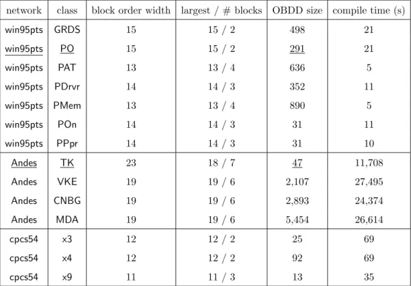
Table 5.3b summarizes compilation experiments we ran on three Bayesian Network classifiers using leaf nodes as feature variables. For each network we included a number of classifiers, each corresponding to one root of the network, using a threshold of 12. Table 5.2 provides similar results on two other networks, except in this case we sampled some of the leaf nodes to include as feature variables (the networks were too large to fully compile). Inference calls were performed using the SamIAm library [Dar].
The sizes of the resulting OBDDs are quite small. For example, the size of the OBDD of the Andes classifier with root ValueKnownEq(VKE) is less than 1% of the state space size given by the block order width. The limiting factor for the compilation algorithm is the
Table 5.1: win95pts has 76 nodes, 16 feature variables and width 9. Andes has 223 nodes, 24 feature variables and width 18. cpcs54 has 54 nodes, 13 feature variables and width 14. Width refers to the network tree-width, approximated by the minfill heuristic.
network class block order width largest / # blocks OBDD size compile time (s)
win95pts GRDS 15 15 / 2 498 21 win95pts PO 15 15 / 2 291 21 win95pts PAT 13 13 / 4 636 5 win95pts PDrvr 14 14 / 3 352 11 win95pts PMem 13 13 / 4 890 5 win95pts POn 14 14 / 3 31 11 win95pts PPpr 14 14 / 3 31 10 Andes TK 23 18 / 7 47 11,708 Andes VKE 19 19 / 6 2,107 27,495 Andes CNBG 19 19 / 6 2,893 24,374 Andes MDA 19 19 / 6 5,454 26,614 cpcs54 x3 12 12 / 2 25 69 cpcs54 x4 12 12 / 2 92 69 cpcs54 x9 11 11 / 3 13 35
compilation time, which depends on the treewidth of the network and scales exponentially with respect to the largest block. The treewidth affects the time of each inference call, and the largest block bounds the number of inference calls made by the compilation algorithm. For example, the two emdec6g experiments in Table 5.2 with 27 and 30 feature variables differ only by 2 in block order width. But, since they differ by 11 in the largest block, we notice a large jump in the compilation time for these two experiments (two orders of magnitude). On the other hand, the experiment with 30 and 33 feature variables also differ by 2 in block order width. Since their largest blocks differ only by 2, the compilation times are comparable (factor of 2). The OBDD size and compilation time are also significantly affected by the threshold of the classifier. A heavily biased threshold can lead to a very small OBDD and a short compilation time, while a balanced threshold generally leads to larger OBDDs.
Table 5.2: Network tcc4ehas 98 nodes and width 10. Network emdec6g has 168 nodes and width 7. We use t27 as the class node for tcc4e, and x29 as the class node for emdec6g.
network # feature variables block order width largest / # blocks OBDD size compile time (s)
tcc4e 21 15 11 / 7 167 4 tcc4e 26 19 14 / 8 930 11 tcc4e 30 30 20 / 6 3,057 1,873 tcc4e 37 37 25 / 8 10,442 39,705 tcc4e 38 38 26 / 8 22,508 91,332 emdec6g 24 24 7 / 13 115 6 emdec6g 27 27 10 / 10 122 11 emdec6g 30 29 21 / 7 4,154 2,487 emdec6g 33 31 22 / 8 3,855 5,308
5.2
Bayesian Network Classifier Case Study
We illustrate the utility of our compilation algorithm by showing how the resulting OBDDs can be used to explain and verify a given classifier. We consider two networks from the literature: win95ptsand Andes; see Table 5.3b. We treat each network as a set of classifiers, taking each root node as a class variable. We treat each leaf node as a feature variable, and use a threshold of 12.
We compile an OBDD for each classifier and then explain their decisions using two types of explanations shown in Chapter 4: minimum cardinality (MC) explanations and prime implicant (PI) explanations [SCD18b].
The win95pts network is used to diagnose why a printing job has failed [BH96]. It has 76 binary variables, 16 of which are leaves which we take as the feature variables of the classifier. One of its root nodes PtrOffline (PO) represents a failure mode (the printer is offline), and has two states: Online (0) and Offline (1). An instance is classified positively if the the probability of being Offline is ≥ 1
2. We first consider a positively classified instance
(indicating a printing failure) that sets 7 of 16 feature variables as 1. The unique MC-explanation for this decision consists of a single feature variable set to 1: the printer icon