American University in Cairo American University in Cairo
AUC Knowledge Fountain
AUC Knowledge Fountain
Theses and Dissertations 2-1-2016
GAdaboost: Accelerating adaboost feature selection with genetic
GAdaboost: Accelerating adaboost feature selection with genetic
algorithms
algorithms
Mai Tolba
Follow this and additional works at: https://fount.aucegypt.edu/etds
Recommended Citation Recommended Citation
APA Citation
Tolba, M. (2016).GAdaboost: Accelerating adaboost feature selection with genetic algorithms [Master’s thesis, the American University in Cairo]. AUC Knowledge Fountain.
https://fount.aucegypt.edu/etds/553
MLA Citation
Tolba, Mai. GAdaboost: Accelerating adaboost feature selection with genetic algorithms. 2016. American University in Cairo, Master's thesis. AUC Knowledge Fountain.
https://fount.aucegypt.edu/etds/553
This Thesis is brought to you for free and open access by AUC Knowledge Fountain. It has been accepted for inclusion in Theses and Dissertations by an authorized administrator of AUC Knowledge Fountain. For more information, please contact [email protected].
The American University in Cairo
School of Science and Engineering
GAdaboost: Accelerating Adaboost Feature
Selection with Genetic Algorithms
A Thesis Submitted to the Department of Computer Science and Engineering in Partial Fulfillment of the Requirements for the Degree of Master of Science
By
Mai Mohamed Tolba
Under The Supervision ofProf. Mohamed Moustafa
ii
ACKNOWLEDGEMENTS
In the name of Allah the most gracious and most merciful
I would like to thank my supervisor Dr. Mohamed Moustafa, for his continuous support and guidance throughout this project. It was really an honor to be taught by such a great professor. I would also like to express my gratitude to my thesis committee members Dr. Amr Gonied and Dr. Hazem Abbas for their helpful feedback.
I would like to thank my father Prof. Mohamed Tolba for his constant guidance, support and encouragement. My mother Galila for her endless love and care. My brother Ahmed for his guidance. My sister Amal, my cousin Aeysha, my sister in law Ghada, my best friend Dalia and my husband Tarek for always being there for me and pushing me to do my best. Without you all this thesis would have not been complete.
iii
ABSTRACT
Throughout recent years Machine Learning has acquired attention, due to the abundant data. Thus, devising techniques to reduce the dimensionality of data has been on going. Object detection is one of the Machine Learning techniques which suffer from this draw back. As an example, one of the most famous object detection frameworks is the Viola-Jones Rapid Object Detector, which suffers from a lengthy training process due to the vast search space, which can reach more than 160,000 features for a 24X24 image. The Viola-Jones Rapid Object Detector also uses Adaboost, which is a brute force method, and is required to pass by the set of all possible features in order to train the classifiers.
Consequently, ways for reducing the whole feature set into a smaller representative one, eliminating those features that have non relevant information, were devised. The most commonly used technique for this is Feature Selection with its three categories: Filters, Wrappers and Embedded. Feature Selection has proven its success in providing fast and accurate classifiers. Wrapper methods harvest the power of evolutionary computing, most commonly Genetic Algorithms, in finding the set of representative features. This is mostly due to the Advantage of Genetic Algorithms and their power in finding adequate solutions more efficiently.
In this thesis we propose GAdaboost: A Genetic Algorithm to accelerate the training procedure of the Viola-Jones Rapid Object Detector through Feature Selection. Specifically, we propose to limit the Adaboost search within a sub-set of the huge feature space, while evolving this subset following a Genetic Algorithm. Experiments demonstrate that our proposed GAdaboost is up to 3.7 times faster than Adaboost. We also demonstrate that the price of this speedup is a mere decrease (3%, 4%) in detection accuracy when tested on FDDB benchmark face detection set, and Caltech Web Faces respectively.
iv
TABLE OF CONTENTS
Contents
ACKNOWLEDGEMENTS ... II
ABSTRACT ... III
TABLE OF CONTENTS ... IV
LIST OF FIGURES ... VII
LIST OF TABLES ... IX
LIST OF ABBREVIATIONS ... X
CHAPTER (1): INTRODUCTION ... 1
1.1 PROBLEM DEFINITION ... 2 1.2 MOTIVATION ... 2 1.2.1 Primary Experiments ... 41.3 ORGANIZATION OF THE THESIS ... 6
CHAPTER (2): BACKGROUND ... 7
2.1 OBJECT DETECTION BACKGROUND ... 7
2.1.1 Viola-Jones Rapid Object Detector ... 7
2.2 ENHANCEMENTS OVER VIOLA-JONES ... 12
2.2.1 The use of SVMs and new stopping criteria ... 12
2.2.2 Increasing Haar Features ... 13
2.3 FEATURE SELECTION. ... 15 2.3.1 Filters ... 15 2.3.2 Wrappers ... 16 2.3.3 Embedded ... 16 2.4 GENETIC ALGORITHMS ... 17 2.4.1 Overview ... 17 2.4.2 GA Details ... 19 2.4.3 Strength of GAs ... 24
2.5 FEATURE SELECTION WITH GAS ... 27
2.5.1 Work that utilizes GA with feature selection. ... 27
v
CHAPTER (3): PROPOSED APPROACH ... 30
3.1 OPENCV ... 30 3.2 GADABOOST OVERVIEW... 31 3.3 GADETAILS ... 35 3.3.1 Initial population ... 35 3.3.2 Chromosome Representation ... 35 3.3.3 Fitness Function ... 36 3.3.4 Selection Mechanism ... 37 3.3.5 Crossover ... 37 3.3.6 Mutation ... 38
CHAPTER (4) EXPERIMENTS ... 39
4.1 TRAINING ... 39 4.1.1 Positive images ... 39 4.1.2 Negative images ... 40 4.1.3 Training Parameters. ... 404.1.4 Resultant trained classifier ... 42
4.2 TESTING ... 43
4.2.1 Datasets ... 43
4.2.2 Detection with OpenCV. ... 44
4.2.3 Evaluation Tools ... 45
4.3 INDIVIDUAL AND POPULATION FITNESS ... 47
4.3.1 Objective ... 47
4.3.2 Method ... 47
4.3.3 Results ... 47
4.3.4 Discussion ... 47
4.4 POPULATION SIZE VERSUS TRAINING TIME ... 48
4.4.1 Objective ... 48 4.4.2 Method ... 48 4.4.3 Results ... 48 4.4.4 Discussion ... 49 4.5 BASELINE ... 49 4.5.1 Objective ... 49 4.5.2 Method ... 49 4.5.3 Results ... 49 4.5.4 Discussion ... 51 4.6 GADABOOST 20 ITERATIONS ... 51 4.6.1 Objective ... 51 4.6.2 Method ... 52 4.6.3 Results ... 52 4.6.4 Discussion ... 54 4.7 GADABOOST 50 ITERATION ... 55 4.7.1 Objective ... 55 4.7.2 Method ... 55 4.7.3 Results ... 56 4.7.4 Discussion ... 58
4.8 TRAINING SPEED VERSUS ACCURACY ... 59
vi 4.8.2 Results ... 59 4.8.3 Discussion ... 62
CHAPTER (5): CONCLUSIONS ... 64
5.1 CONTRIBUTIONS ... 64 5.2 FUTURE WORK ... 65REFERENCES ... 66
vii
LIST OF FIGURES
Figure1-1: The effect of varying the image size on the number of features ... 4
Figure 1-2: The effect of increasing Haar feature types on the total number of features per a 24x24 image ... 5
Figure 2-1: Haar features relative to the enclosing detection window (Viola & Jones, 2001) ... 8
Figure 2-2: Integral image illustration(Viola & Jones, 2001)... 9
Figure 2-3: Adaboost Algorithm(Viola & Jones, 2001) ... 10
Figure 2-4 Schematic description of a detection cascade(Viola & Jones, 2001) ... 11
Figure 2-5: Roc Curve for detector on MIT+CMU dataset (Viola & Jones, 2001)... 12
Figure 2-6 Object detection average precision on selected objects (top 40 in 113 test image)(Q. Li et al., 2012) ... 13
Figure 2-7 Extended set of Haar features black and white regions have negative and positive weights (Lienhart & Maydt, 2002) ... 14
Figure 2-8: Basic versus extended features set. (Lienhart & Maydt, 2002) ... 15
Figure 2-9: How GAs Work (Lee & Lee, 2014) ... 19
Figure 2-10: Single point Crossover (Hasançebi & Erbatur, 2000) ... 19
Figure 2-11: Two-point crossover (Hasançebi & Erbatur, 2000) ... 20
Figure 2-12: Uniform crossover(Hasançebi & Erbatur, 2000) ... 20
Figure 2-13 Tournament selection(Noraini & Geraghty, 2011) ... 21
Figure 2-14 Roulette wheel selection (Noraini & Geraghty, 2011) ... 23
Figure 2-15: Comparison of mean cutsizes (Manikas & Cain, 1996) ... 26
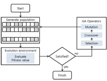
Figure 3-1 GAdaboost algorithm flowchart ... 32
Figure 3-2 Population illustration ... 35
viii
Figure 3-4 GAdaboost crossover illustration ... 38
Figure 4-1 Positive training images ... 40
Figure 4-2 Negative images samples ... 40
Figure 4-3 Opencv_traincascade parameters ... 41
Figure 4-4 Resultant cascade classifier ... 42
Figure 4-5 Example of a stored stage of resultant classifier ... 43
Figure 4-6 Example of annotated FDDB dataset(Jain & Learned-Miller, 2010). ... 44
Figure 4-7 Best individual fitness and average population fitness over 50 iterations . 47 Figure 4-8 Population size vs training time. ... 48
Figure 4-9 Examples of detection of baseline on images ... 50
Figure 4-10: Baseline performance on FDDB dataset ... 50
Figure 4-11: Baseline performance on the Caltech dataset ... 51
Figure 4-12: Examples of detection of Gadaboost20 on images ... 53
Figure 4-13: ROC curve of multiple GAdaboost20 Classifiers on FDDB ... 54
Figure 4-14: ROC curve of multiple GAdaboost20 Classifiers on Caltech... 54
Figure 4-15: Example of detections of GAdaboost50 ... 57
Figure 4-16: ROC curve of multiple GAdaboost50 Classifiers on FDDB ... 57
Figure 4-17 ROC curve of multiple GAdaboost50 Classifiers on Caltech ... 58
Figure 4-18 Training time in minutes of each of the experiments. ... 60
Figure 4-19 Y error bars for all the runs of the 20 iterations GAdaBoost on FDDB. . 60
Figure 4-20: Y error bars for all the runs of the 50 iterations GAdaBoost on FDDB . 61 Figure 4-21: Y error bars for all the runs of the 20 iterations GAdaBoost on Caltech Web Faces. ... 61
Figure 4-22: Y error bars for all the runs of the 50 iterations GAdaBoost on Caltech Web Faces. ... 62
ix
LIST OF TABLES
Table 1-1 Comparison between Brute Force and GA in TSP ... 6
Table 2-1: Number of features inside a 24X24 image for each prototype (Lienhart & Maydt, 2002) ... 14
Table 2-2: Summary of feature selection techniques ... 17
Table 2-3 Discrimination results on synthetic images (Ayala-ramirez et al., 2006) ... 24
Table 2-4 Discrimination results on natural images (Ayala-ramirez et al., 2006) ... 24
Table 2-5: comparison on Caltech dataset to other methods ... 25
Table 3-1 Comparison of OpenCV Application used to train a cascade classifier. ... 31
Table 4-1 Training time for each run of training GAdaboost 20 ... 52
Table 4-2 Training time for each run of training GAdaboost 50 ... 56
Table 4-3 Summary of performance of the baseline, GAdaboost50, and GAdaboost20 ... 63
x
LIST OF ABBREVIATIONS
ACO Ant Colony Optimization CV Computer Vision
EC Evolutionary Computing EA Evolutionary Algorithms FDDB Face Detection Database GA Genetic Algorithms HOG Histogram of Gradients LBP Local Binary Patterns ML Machine Learning
OpenCV Open Source Computer Vision Library PSO Particle Swarm Optimization
ROC Receiver Operator Curve SFS Sequential Forward Selection SBS Sequential Backward Selection SVM Support Vector Machine TBB Threading Building Blocks TSP Travelling Salesman Problem
1
CHAPTER (1): INTRODUCTION
Machine learning and training require large feature sets, which can be time consuming to explore. With the advancements in this field the need for algorithms to decrease the training time arises. Genetic Algorithms (GA) have proven their strength in solving problems like the aforementioned one, especially those concerned with exploring large search spaces and providing acceptable results in a significantly reduced amount of time than that of the brute force manner. Many researches have explored the use of GA in time consuming tasks like Feature Selection, which aims to choose a representative small sub-set of features from the whole set of features (B Xue, Zhang, Browne, & Yao, 2016).
Object detection lies in the set of machine learning techniques that require a huge search space for training, thus their training is time consuming. Object detection is concerned with detecting whether an object is present in a given image and where it lies in this image. It has many applications including but not limited to, face detectors in all modern state of the art cameras, automotive safety, video indexing, image classification, surveillance and content-based image retrieval (Lillywhite, Lee, Tippetts, & Archibald, 2013).
A lot of research has been applied to this area, due to its complex nature as detection is hard to achieve in different light conditions, occlusion and the angle in which the object appears in the image (Lienhart & Maydt, 2002; Lillywhite et al., 2013; Viola & Jones, 2001). Researchers have been trying to implement efficient high speed detectors that work in real time and have a high percentage of accuracy. Though the Viola-Jones detector has reached an impressive detection speed, it still consumes a lot of time in training. Viola-Jones uses Adaboost, a type of boosting algorithms, to select and combine weak classifiers to form a strong one. Adaboost is simple and adaptive (Dezhen & Kai, 2008), yet it operates in a brute force manner, passing by the set of all features multiple times. This can be very time consuming, as the search space consists of a set of more than 160,000 features for a 24X24 image.
This thesis is multi-disciplinary, as it deals with three sub-research areas in Computer Science. The three main areas are Computer Vision (CV), Machine Learning (ML) and Statistics, and Evolutionary Computing (EC). This thesis’s main focus is on Object detection which lies under CV, Boosting and Feature Selection which is a sub-area of ML and Genetic Algorithms with is a famous algorithm in EC. In brief this work aims towards enhancing the training time taken by the Adaboost algorithm through Feature Selection using Genetic
2
Algorithms. Specifically it aims to speed up the training process of the Viola-Jones Rapid Object Detector by finding a small set of representative features to be provided to the Adaboost algorithm, instead of the original method of going through the set of all possible features in a brute force manner.
1.1
Problem Definition
Having Robust and efficient detectors has become the goal of many research over many years. An ideal detector can be described as one that is both efficient and provides plausible results. A lot of research has been done in order to enhance several machine learning techniques and try to reach the previously mentioned goal of ideal detectors.
Though Boosting algorithms like Adaboost are simple and effective, they suffer from lengthy training processes due to their brute force nature. With the advancement of Machine Learning and the abundance of data in recent years (Yusta, 2009), the drawback of these algorithms becomes more apparent, as the dimensionality and the volume of data directly affect the training time. For example, in the training of the Viola-Johns Rapid Object detector, the Adaboost algorithm goes through the set of all possible features in a brute force manner, for the training of each weak classifier. This can be very time consuming, as the search space consists of a set of more than 160,000 features for a 24X24 image (Viola & Jones, 2001). Some of the formerly mentioned features are non-representative as they have poor predictive power of the object’s existence in this image. Selecting a representative set of features and discarding the non-useful ones can be achieved through Feature Selection. Feature selection, allows for the decrease of the search space with minimum loss of quality, as it focuses on eliminating those features that are not useful when solving the problem at hand. Applying this concept to the Adaboost algorithm will help in overcoming the drawback of its lengthy training process while benefiting from its simplicity and adaptively.
1.2
Motivation
The Viola-Jones object detector uses a cascaded stage classifier in order to rapidly detect objects. However, the training of this classifier is time consuming, since the training algorithm utilized is Adaboost which works by going through the set of all possible features to
3
evaluate each feature in a brute force manner to choose one weak classifier. This process takes place multiple times as the essence of boosting is to combine multiple weak classifiers to get a strong one. The cascaded structure makes training even slower as the previously mentioned process is repeated for each stage of the cascaded classifier. The number of times the Adaboost algorithm passes through the set of all possible features to train a cascade classifier, can be obtained by summing up the number of weak classifiers in all the stages as shown in Equation 1.1, where WC is the number of weak classifiers per stage, and n is the number of stages in the cascade classifier.
𝑖𝑡𝑒𝑟𝑠 = ∑ 𝑊𝐶𝑖 𝑛
𝑖=0
(1.1)
Examining the set of all possible features multiple times can be analogous to expanding the feature set. In order to have a deeper understanding of the effects of repeating the number of iterations a look at how much the feature set expands is necessary. The total number of features examined in training a cascade classifier is obtained by multiplying the number of iteration done by the Adaboost algorithm by the total number of features in the original feature set as shown in Equation 1.2, where TF is the total number of features examined, iters in the number of times the Adboost passes by the original search space (which can be obtained from Equation 1.1), and osp is the number of features in the original search space
𝑇𝐹 = 𝑖𝑡𝑒𝑟𝑠 ∗ 𝑜𝑠𝑝 (1.2)
As an example, if we built a simple 5 stage classifier and the number of features are 10, 15, 20, 25, 30 in stages 1, 2, 3, 4 and 5 respectively, then the total number of times the Adaboost passed by the set of all possible features (the original search space) in the trainng phase can be calculated by summing up the number of features, i.e. 10+15+20+25+30 which is equal to 100 in this final trained classifier, which is analogous to an increased search space by a 100 times, as the Adaboost would have passed by 160,00000 features if the original search space had 160,000 features (160,000 X 100 from Equation 1.2)
In conclusion, by eliminating the unnecessary features, the time taken to train a cascade classifier can be significantly reduced. This can be achieved by the means of Feature Selection, where the best features are chosen and the unnecessary ones are discarded. Feature Selection can be achieved by exploiting GAs, since GAs are widely used heuristics in Feature Selection (Tsai, Eberle, & Chu, 2013). Another motivation for using GA with Feature Selection is that
4
inducing GAs and Feature Selection mechanisms have been continuously studied for decades (Chaaraoui & Flórez-Revuelta, 2013; Yusta, 2009) and have proven to be successful.
1.2.1
Primary Experiments
This section provides 2 experiments to support the motivation of this work. It shows evidence of how vast the search space of features can be by examining the effect of increasing Haar feature types on the total number of features and the effect of image size of the number of features in the search space. Moreover, an experiment was done to compare the brute force technique versus the GAs in solving the Travelling Salesman Problem.
1.2.1.1
Number of Features Per image
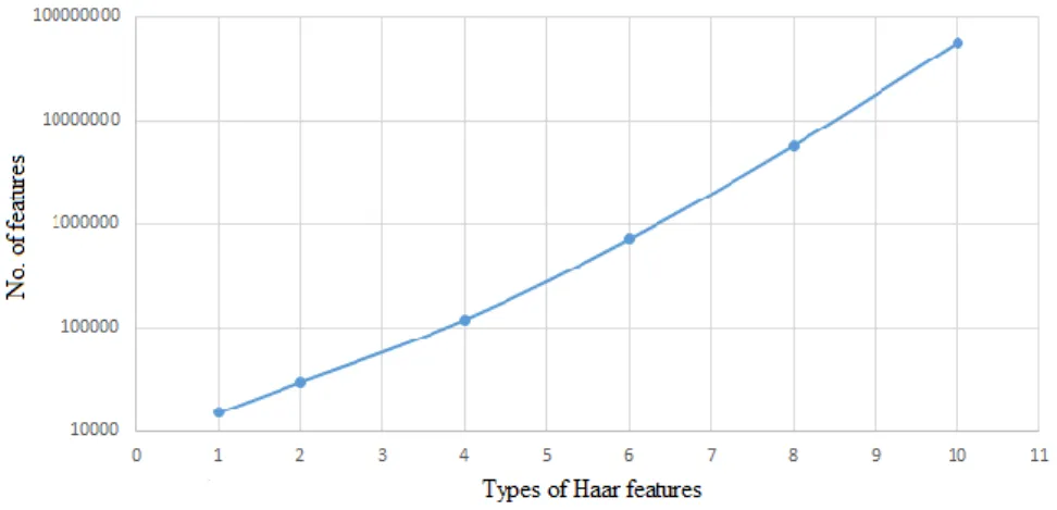
The main problem to be dealt with in order to enhance the performance of the Viola-Jones detector, is the vast search space. To give an idea of how vast this search space can get; a simple experiment has been carried out. This experiment calculates the number of features (the search space) once when varying the image dimensions and another when increasing the types of Haar features. This experiment considers getting all possible sizes of each feature and all possible positions by shifting the window one pixel. Figure1-1 shows the exponential growth of the search space when increasing the image dimensions. Figure 1-2 also shows the growth of the search space by increasing the types of Haar features used.
5
Figure 1-2: The effect of increasing Haar feature types on the total number of features per a 24x24 image
1.2.1.2
Performance of GA in Travelling Salesman Problem (TSP)
With a vast search space the main problem is time. It’s a time consuming process to go through the search space one by one in a brute force manner (as done by the original Viola-Jones implementation). The former point is the motive for this work, since Genetic algorithms in general are efficient in searching large spaces (Lillywhite et al., 2013). To further show the effectiveness of GA on speed and accuracy an experiment was conducted. The famous Travelling Salesman Problem (TSP) has been examined once using brute force and once using Genetic Algorithms (implementation used was done by (Jacobson, 2012)). The Travelling Salesman Problem is concerned with finding the shortest route of a journey between given countries. For this experiment the same 9 countries have been used for both the GA and the brute force methods. The brute force method is done by exploring all the possible routes (which are 9! (362880) routes) in this case, then choosing the shortest one. The results of the experiment show that the GA achieved a comparable accuracy by evaluation a 100 generations in only 5.9% of the time taken by the brute force method. Table 1-1 shows the exact results of the timing and the shortest distance found by both the brute force and the GA.
6
Table 1-1 Comparison between Brute Force and GA in TSP
1.3
Organization of the Thesis
The rest of the thesis is organized as follows: Chapter 2 provides a comprehensive background on the main topics covered in this thesis, like the Viola-Jones Rapid Object Detector and the enhancements done over their work. Basic Genetic Algorithm concepts are discussed and previous work proving their strength is reviewed. Feature Selection concepts and terminology are provided. Finally previous work that utilizes Genetic Algorithms in Feature Selection is examined. Chapter 3 explains the proposed method, while providing details on implementation and tools used. Chapter 4 explains the experimental setup and details of the experiments provided. Chapter 5 concludes the thesis and discusses future work.
7
CHAPTER (2): BACKGROUND
This chapter provides background on the three main concepts used in this work, by discussing the Viola-Jones object detector. Details on Viola-Jones Rapid Object Detector and some of the research that aims to enhance this detector are provided, since the enhancement of the training time of this detector is the main objective of this work. After that an overview on GAs and their main concepts are discussed, with some previous work that sheds light on the success and wide usage of these algorithms. Feature Selection is then mentioned, with their categorization and main concepts. Finally previous work that combined both Feature Selection and Genetic Algorithm is presented.
2.1
Object Detection background
As this research area is relatively new, as mentioned by Hjelmas et al. (Hjelmås & Low, 2001) that the face detection problem has attained little attention before 1998 (Amit, Geman, & Jedynak, 1998). This is apparently not the case now since this area has gained more attention by the time that Herman et al. conducted their survey (Hjelmås & Low, 2001). Since then many researchers have focused on this area. Scientists have been working and contributing to detectors over the past decade. Viola-Jones is an example of widely used detectors. This section will provide a brief introduction on this detectors; since it provides the basis for this research.
2.1.1
Viola-Jones Rapid Object Detector
Viola et al. devised a rapid object detector, with 3 major contributions. The first contribution is that they provided an image representation called the integral image that allows the features to be evaluated fast. Their second contribution is that they devised a method for construction of the classifier though the selection of important features using Adaboost. Their third contribution is successively combining complex classifiers in a cascade structure which allows for fast detection on the test images (Viola & Jones, 2001).
The basic and main 3 components of the Viola-Jones classifiers are: The Haar features
Integral Image Adaboost
8
2.1.1.1
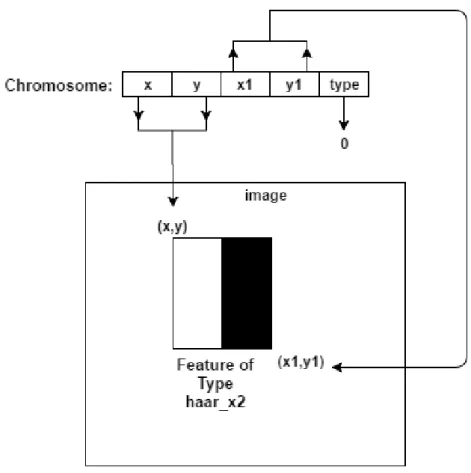
Haar Features
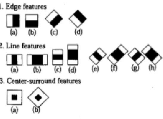
The use of features has proven to be better than using pixels, as features proved a set of comprehensive information that can be learned by machine learning algorithms. Features reduce the in-out class variability compared to that of the raw pixels (Lienhart & Maydt, 2002; Viola & Jones, 2001). This is in general, a clear incentive that provides more reasons to use features instead of raw data. For this particular system a critical issue is speed of calculation and the features operate much faster than raw pixels (Viola & Jones, 2001). The Haar features used are shown in Figure 2-1. The value of the feature is obtained by subtracting the sum of the pixels in the white region from the sum of the pixels in the black region. The four features used are those that are best for distinguishing upright front-facing faces. For example, feature (c) in Figure 2-1 can detect the nose area as its lighter than the eyes and feature (a) can detect eyes as the eyes region is darker than the region under it (Viola & Jones, 2001). For each image, each of the four Haar features is computed in all possible sizes and all possible locations which provide a huge number of features.
Figure 2-1: Haar features relative to the enclosing detection window (Viola & Jones, 2001)
2.1.1.2
Integral Image
Viola et al. introduced a new concept called the integral image in order to facilitate the computations of features since there are a lot of them. Any position in the integral image x, y is the sum of all the pixels above and to the left of x, y inclusive (Viola & Jones, 2001). Figure 2-2 shows the illustration of the integral image. For example, the value of location 1 in the
9
integral image is the sum of pixel values of rectangle A. Similarly the value of location 2 in the integral image is the sum of pixel values of rectangle A and B. The value at location 3 is A+ C. As for the sum of pixel values in rectangle D, it can be obtained by subtracting the value at location 2 and 3 from the value at location 4 then adding the value at location 1, as its going to be subtracted twice while subtracting both 2 and 3, since the value at 1 is contained in both 2 and 3. The equation of obtaining the pixel values at rectangle D is 4 +1- (2+3). The integral image reduces the calculation cost of pixels as it can calculate the sum of pixel values at any given rectangle by 4 array accesses at most.
Figure 2-2: Integral image illustration(Viola & Jones, 2001)
2.1.1.3
Boosting
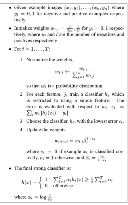
The authors chose Adaboost as a method to obtain their strong classifier. “Boosting is an approach to machine learning based on the idea of creating a highly accurate prediction rule by combining many relatively weak and inaccurate rules.” (Schölkopf, Luo, & Vovk, 2013). Adaboost , which was proposed by Freund and Schapire (Freund & Schapire, 1995), has been the first practical boosting algorithm and is still widely used in many applications (Schölkopf et al., 2013). Adaboost is simple and adaptive (Dezhen & Kai, 2008) yet it operates in a brute force manner, passing by all the set of features multiple times. Figure 2-3 explains the Adaboost algorithm, where each round of boosting selects one feature from the set of all possible features.
10
Figure 2-3: Adaboost Algorithm(Viola & Jones, 2001)
The general idea of the algorithm works as follows: For a number of iterations T:
Pass through the set of all possible features and calculate the error of each one on the given images.
Choose the best feature (the one with the lowest error) as the first weak classifier.
Update the sample images and their corresponding weights, by putting more weights on the wrongly classified images.
11
Go through the next iteration, until it finds the set of best features to be used in classification.
As shown from Figure 2-3 the weights are updated as a function of the error produced by the chosen classifier. In other words, the samples that has been misclassified by the chosen classifier are given more weight. These weights are used to inform the training of the weak classifiers i.e, the classifier that correctly classifies samples with higher weights are considered to be of better performance than the other classifiers.
2.1.1.4
Cascade Classifier
One of the important contributions of (Viola & Jones, 2001) is the cascaded classifier. This structure of the classifier allows for better accuracy while radically reducing the time consumed in detection (Viola & Jones, 2001). The cascaded classifier is a stage classifier where the thresholds vary. The first stages have a low threshold, thus detecting all the true positive while eliminating the strong negatives, before the more complex classifiers are called to achieve less false positives. Figure 2-4 provides a description of this classifier.
Figure 2-4 Schematic description of a detection cascade(Viola & Jones, 2001)
From Figure 2-4 it is clear that a series of classifiers are applied to every sub-window. The initial classifier is able to eliminate a huge number of negative examples with little processing. The following stages of classifiers then eliminate additional negatives, yet they apply more computations. After several stages of processing the number of sub-windows are drastically reduced (Viola & Jones, 2001).
12
2.1.1.5
Results
The resultant classifiers, on which the authors of (Viola & Jones, 2001) trained and based their experiments on is a cascaded one of 38 layers. The training set consisted of a set of 24X24 pixel images, of which 4916 faces and 9544 non faces. Within these non faces there are 350 million sub-windows and the total number of features is 6061. This detector was tested on the MIT+CMU frontal faces test. This set has a total of 130 images with 507 labeled frontal faces. The results are shown in the Receiver Operator Curve (ROC) in Figure 2-5.
.
Figure 2-5: Roc Curve for detector on MIT+CMU dataset (Viola & Jones, 2001)
2.2
Enhancements over Viola-Jones
Some of the researchers used the Viola-Jones algorithm as a base for their research then proposed and implemented their concepts to provide even more powerful detectors. Li et al. proposed new enhancements that include SVMs and stopping criteria to detect more objects instead of just frontal-upright faces. Lienhart et al. proposed the increase of Haar features used. This section will give more details about both approaches.
2.2.1
The use of SVMs and new stopping criteria
Li et al (Q. Li, Niaz, & Merialdo, 2012) have achieved 3 major contributions. They used multiple feature images instead of just gray ones used by Viola-Jones, They devised a way to avoid the non-converging in training the classifier. They also outputted a weighted value as a confidence measure to whether the test image contains the desired objects or not.
13
The training data is preprocessed and a set of 6 image features are produced, the 6 types are: Gray image, Local Binary Patterns (LBP), EDGE, L-channel, A-channel and B-channel images. They tackled the problem of the non-converging training set in the cascaded classifier since the stopping criteria is a preset false alarm rate which sometimes is never reached. In order to fix this, they introduced a new stopping criterion, which is the maximum variance ratio (R) between the score of the positive and the negative training images. The main idea is to separate the positive and negative as much as possible and keep the inner variance of each class small. The score is defined as “the stage sum of the last stage classifier of a survived image patch. Stage sum is the cumulative sum of Haar like features convolved with the image patch (Q. Li et al., 2012). If R keeps increasing the training continues, the training classifier will converge since R will not be increasing all the time. As for the detection part, a key point based SVM is incorporated to get a confidence measure (to weigh the output score). The authors tested their algorithm on the TRECVID 2011 development dataset, they chose four objects which are: Computers, Scene_Text, Telephone and Hand. In all of these categories their algorithm performed much better than the Viola-Jones implementation in OpenCV. The results can be seen in Figure 2-6.
Figure 2-6 Object detection average precision on selected objects (top 40 in 113 test image)(Q. Li et al., 2012)
2.2.2
Increasing Haar Features
The authors of (Lienhart & Maydt, 2002) approach in enhancing the Viola-Jones Rapid Object Detector differs from the approach pursued by the authors of (Lienhart & Maydt, 2002). They wanted to enhance Viola-Jones by increasing the Haar features to more than the 4 used in the original work. They used 45 degrees rotation of feature that adds domain knowledge to the learning framework. These features can be seen in Figure 2-7.
14
Figure 2-7 Extended set of Haar features black and white regions have negative and positive weights (Lienhart & Maydt, 2002)
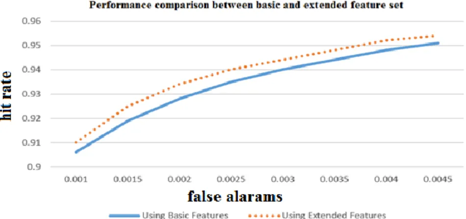
Increasing the type of features from 4 to 14 substantially increased the number of generated features per image. Table 2-1 gives a summary of the number of features inside a 24x24 image window per feature prototype from Figure 2-7. The upright features can be computed fast by the integral image (Lienhart & Maydt, 2002). As for the rotated ones the authors created a rotated summed area table to enable them to calculate the value of the rotated features fast. The results shows that with these extended set of features the classifier performs better than the original one that had only 4 features, they also had comparable computation complexity. Figure 2-8 shows the ROC curve of the 2 classifiers with 12 stages.
15
Figure 2-8: Basic versus extended features set. (Lienhart & Maydt, 2002)
2.3
Feature Selection.
A feature can be defined as measurable property of the data being observed (Chandrashekar & Sahin, 2014). Feature Selection is the process of reducing the whole search space into a sub-set of relevant features. This helps in removing noise and irrelevant features reducing time while providing good prediction results (Chaaraoui & Flórez-Revuelta, 2013; Chandrashekar & Sahin, 2014; Jeong, Shin, & Jeong, 2014; Lee & Lee, 2014; Liang, Tsai, & Wu, 2014; Oreski & Oreski, 2014; Santana, Silva, Canuto, Pintro, & Vale, 2010; Vignolo, Milone, & Scharcanski, 2013; Xia, Zhuang, & Yu, 2014; B Xue et al., 2016; Bing Xue, Fu, & Zhang, 2014; Yusta, 2009). The need for feature selection methods arose due to the availability of high dimensional data with hundreds or thousands of attributes. In other words Feature Selection methods are ways to solve the curse of dimensionality (Powell, 2007).
Feature Selection techniques are divided into 3 main categories which are Wrappers, Filters and Hybrid (Embedded) methods. (Chaaraoui & Flórez-Revuelta, 2013; Liang et al., 2014; Oreski & Oreski, 2014; Santana et al., 2010; Vignolo et al., 2013; Yusta, 2009). Table 2-2 provides a summary for these three categories.
2.3.1
Filters
Filter techniques rely on the intrinsic properties of the data without involving a classification technique (Oreski & Oreski, 2014). They use variable ordering techniques as criteria for selection by ordering. Variables that are below a certain threshold and excluded from the original variable set (Chandrashekar & Sahin, 2014). A basic criteria of the chosen
16
feature is to have useful information about the classes of the data. This property can be called feature relevance, which is the ability of this feature to discriminate between classes. Feature reference can be defined as “feature can be regarded as irrelevant if it is conditionally independent of the class labels.” (Chandrashekar & Sahin, 2014). Some examples used for filter techniques are: Correlation criteria, mutual information (Chandrashekar & Sahin, 2014).
The advantages of the filter methods are: That they are computationally efficient, avoids overfitting and has proven to work well on certain datasets (Chandrashekar & Sahin, 2014). They don’t rely on learning algorithms which are biased and change the data to fit the learning algorithm. The disadvantages of some of these methods are that they don’t consider the feature in relation with other features. In other words, features that are not informative on their own but give valuable information when combined with other features might be disregarded. (Chaaraoui & Flórez-Revuelta, 2013; Chandrashekar & Sahin, 2014; Oreski & Oreski, 2014; Santana et al., 2010; B Xue et al., 2016).
2.3.2
Wrappers
Wrapper methods use classifier predictions as a fitness measure for the sub-set of features (Chaaraoui & Flórez-Revuelta, 2013; Chandrashekar & Sahin, 2014; Jeong et al., 2014; Lee & Lee, 2014; Liang et al., 2014; Oreski & Oreski, 2014; Santana et al., 2010; Vignolo et al., 2013; Xia et al., 2014; B Xue et al., 2016; Bing Xue et al., 2014; Yusta, 2009). Since evaluating multiple subsets is an N-P hard problem, Wrappers become computationally expensive especially with large datasets. Wrappers often utilizes metaheuristics like GAs, Particle Swarm Optimization (PSO) and Ant Colony optimization (ACO). Though Wrappers are generally more accurate than Filters, their main drawback is computational complexity since each sub-set of features is passed to a classifier for training and testing to in order to calculate the accuracy (Chaaraoui & Flórez-Revuelta, 2013; Chandrashekar & Sahin, 2014; Oreski & Oreski, 2014; Santana et al., 2010; B Xue et al., 2016). Another drawback of these methods which use classifier prediction as the objective function is that these classifiers are prone to overfitting. Overfitting happens when the classifier lacks the ability for generalization and only acts well on the data used for training. In this case the classifier will be biased and provide poor classification results (Chandrashekar & Sahin, 2014).
2.3.3
Embedded
Embedded methods are hybrid methods that try to combine the advantages of both Wrappers and Filters. It aims to reduce the time taken by wrappers in re-classifying the
sub-17
sets by incorporating the subset selection while training. In (Chandrashekar & Sahin, 2014) some of the embedded methods techniques are provided and discussed.
Table 2-2: Summary of feature selection techniques
Filters Wrappers Embedded
Definition Relies on general properties of data.
Uses machine learning approaches as black boxes to score features.
Combines both the filter and wrapper approach.
Advantages Computationally more efficient in comparison to wrapper approach.
Provides more accurate subsets than filters.
Tries to reduce the time taken by wrappers by including filters in the learning process
Disadvantages Provides worse subsets. Involves computational overhead to score features.
2.4
Genetic Algorithms
This section provides background on Genetic Algorithms (GAs), their techniques and the processes involved such as mutation, crossover and selection methods.
2.4.1
Overview
Genetic Algorithms are heuristic mechanisms that are successful in solving many difficult problems. They can be considered the best solution for high complexity problems such as the combinatorial optimization (Tabassum & Mathew, 2014). GAs are most likely the first Evolutionary Computing (EC) technique to be widely applied to Feature Selection problems (B Xue et al., 2016). Genetic Algorithms (GAs) were first proposed by John Holland (Holland, 1975). They are optimizing procedures that are devised from the biological mechanisms of reproduction and evolutionary science (survival of the fittest) (Andrade & Errico, 2008; Harb & Desuky, 2011; Sun, Bebis, & Miller, 2004). In natural, individuals compete for scarce resources like food and shelter. The best individuals that are suited for this competition survive. Adaptation to the surrounding environment is essential for the survival of a species. The traits that uniquely characterizes the individual determines its chances for survival (Srinivas & Patnaik, 1994). These traits are encoded in each individual as genes. The best genes survive through generations by means of reproduction. In other words, fit genes enable individuals to survive, reproduce, consequently passing on their fit genes to their offspring, which in turn will pass through competition and those who survive will reproduce passing on their genes. This
18
will ensure that over the course of generations, the genes in the offspring are to be refined, providing fitter generations that are more capable of adapting to the environment.
GAs resemble survival of the fitness mechanism as they start with an initial random population that propose solutions to the problem at hand (Mitchell, 1998; Sun et al., 2004). Each individual in the population is encoded (usually as a string of bits) in order to mimic a chromosome. This denotes that the parameters of the problems are joined to form one possible solution chromosome. In order to evaluate the fitness of this individual, it’s associated with a fitness score that governs its ability to survive through generations and breed. This score is provided by an objective that is set and is referred to as a fitness function. The main Idea of GAs is to get those individuals which prove to be promising, pass them on to the reproduction phase where their genes are combined and slightly modified to provide offspring. The fitness score controls the probability of an individual to be chosen; as the selection process usually favors fitter individuals i.e. individuals of a higher fitness score. This means that fitter individuals have the chance to be selected more than once and poorly performing individuals might not be selected at all. This is done several times and finally the fitness of the population should converge to an optimal or a near optimal solution.
The formation of new offspring in the reproduction phase is attained by means of crossover and mutation. Crossover is the process where genes of 2 individuals are combined to form a new individual. Mutation occurs by changing one gene of the produced children from the crossover phase. (Lillywhite et al., 2013). Crossover allows for fast exploration of the search space, while mutation increases the probability of the exploration of all of the search space. In other words, it decreases the probability of having an unexplored solution in the search space.
In brief, the basic operations that guide the GAs search are: Encoding, evaluating, selecting and recombining individuals. These operation are preformed iteratively (Sun et al., 2004). They stop at a predefined stopping criteria or when the given maximum number of iterations is reached. Figure 2-9 explains how GA works.
19
Figure 2-9: How GAs Work (Lee & Lee, 2014)
2.4.2
GA Details
2.4.2.1
Crossover Types
Crossover is the process where fit individuals are combined to form new individuals that will be a part of the next generation. This process helps in the exploration of the search space. Crossover has many forms; the most important ones are discussed in the following subsections.
2.4.2.1.1 One-Point Crossover
One-point crossover is the simplest form of crossover. In this type, a point is chosen randomly and the 2 parent chromosomes are cut at this point. Then the sections after this cut, are exchanged to form the 2 children (Hasançebi & Erbatur, 2000; Magalhães-Mendes, 2013). Figure 2-10 visually illustrates the one-point crossover technique.
20 2.4.2.1.2 Two-Point Crossover
Two-point crossover is when the 2 parents are cut at 2 different points. It is done by either swapping the inner portions (genes between the 2 points) or the outer portion, since both options provide the same results (Hasançebi & Erbatur, 2000; Magalhães-Mendes, 2013). Figure 2-11 illustrates the two point crossover.
Figure 2-11: Two-point crossover (Hasançebi & Erbatur, 2000)
2.4.2.1.3 Multi-point crossover
Multi-point crossover is an extension to the two point crossover where the two parents are cut at 3 or more points and the portions between these points are exchanged. This type of crossover helps the exploration of more parts of the search space (Hasançebi & Erbatur, 2000). 2.4.2.1.4 Uniform Crossover
In this type of crossover a bit mask of the same length of the individual (chromosome) length is randomly created. Each bit of the mask determines the gene would be copied from which parent into the child. 1 means the gene will be transferred from parent number one, 0 indicates that the gene will be copied from parent number two (Hasançebi & Erbatur, 2000). Figure 2-12 illustrates the uniform crossover.
21
2.4.2.2
Selection Mechanisms
Selection mechanisms are crucial as they choose the individuals that will participate in the next generation. If the best individual is always chosen, premature convergence will occur (Andrade & Errico, 2008). Premature Convergence is when a highly fit gene (but not optimal) dominates generations, causing the population fitness to converge to a local maxima. As a form of avoiding this problems many selection techniques where devised.
2.4.2.2.1 Tournament Selection
Tournament selection is the most commonly used selection mechanism, due its simplicity and straight forward implementation (Goldberg & Deb, 1991; Noraini & Geraghty, 2011). It’s achieved by randomly selecting a number of individuals from the population. These individuals compete and the fitter one is chosen to participate in the next generation. The number of competing individuals is called tournament size and is usually set to two (Noraini & Geraghty, 2011). Tournament section gives each individual the chance to participate, thus preserving diversity though this might lead to slower convergence. Tournament selection has several advantages which include efficient time complexity, especially if implemented in parallel, low susceptibility to takeover by dominant individuals and no requirement for fitness scaling or sorting. (Baker, 1985; Goldberg & Deb, 1991; Noraini & Geraghty, 2011). Figure 2-13 shows an illustration of the tournament selection mechanism.
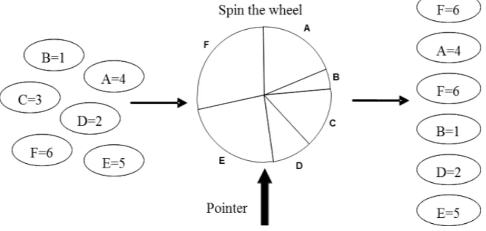
22 2.4.2.2.2 Roulette Wheel Selection
Proportional Roulette Wheel Selection
In proportional Roulette Wheel Selection, the probability of an individual being chosen is directly proportional to its fitness value, i.e the fitter individual has a higher probability of being selected. The probability of choosing a parent is analogous to a roulette wheel and the size of its segments are proportional to each parent’s fitness. Thus parents with higher fitness have larger segments on the roulette wheel, consequently more chance of being chosen. The probability of choosing an individual is calculated by equation (2.1) (Noraini & Geraghty, 2011). Where p is the probability of choosing individual, f is the fitness value of individual. N is the total number of individuals the population.
𝑝𝑖 = 𝑓𝑖 ∑𝑛𝑖=0𝑓𝑖
(2.1)
This type of selection mechanisms gives chance to all of the individuals in the population, preserving the diversity. Yet, it gives higher probability to fittest individuals, which may cause these individuals to dominate populations fast which eventually leads to premature convergence, and loss of genetic diversity. For example if the population contains two fit induvial and the rest of the population has poor fitness, these two fit individuals will dominate the population quickly. On the other hand, if the whole population is of similar fitness, the population will face difficulty in evolving to a better solution since both probabilities of fit and unfit individuals are similar. (Noraini & Geraghty, 2011)
Rank-Based Roulette Wheel Selection
At the beginning the individuals are sorted according to their fitness values, and the probability of one being chosen is based on its rank in the sorted array. Rank based selection is not influenced by “super-individuals” or the spread of fitness values. Rank-based selection depends on a mapping function that maps the indices of the individual in the sorted list according to their fitness values. Thus, the performance of this technique depends heavily on the mapping function
23
chosen. (Noraini & Geraghty, 2011). Figure 2-14 shows the Roulette Wheel selection mechanism.
Figure 2-14 Roulette wheel selection (Noraini & Geraghty, 2011)
2.4.2.2.3 Deterministic Sampling
In deterministic sampling the average fitness of the population is calculated. After that, the fitness value of each individual is divided by the average fitness of the population and the integer part is stored. If the integer is greater than 1, the individual is chosen, else the individual will not be selected to participate in the next generation. The rest of the population size is then filled by choosing individuals with greater fractions. (Andrade & Errico, 2008)
2.4.2.2.4 Stochastic Remainder Sampling
Stochastic random sampling is identical to deterministic random sampling where the individual is chosen based on the integer part resulting from the operation of dividing the individual population by the average population. The rest of the population size is filled by the means of a roulette wheel selection.
2.4.2.3
Mutation
Mutation is another form of exploring the search space, it reduces the probability of having an unexplored solution. Mutation is mainly concerned with changing a one gene of the child produced by the crossover process, according to a preset probability.
24
2.4.3
Strength of GAs
GAs are powerful optimization algorithms that have proven their success in many fields. Tabassum et al. Mentioned that “It was proved that genetic algorithms are the most powerful unbiased optimization techniques for sampling a large solution space” (Tabassum & Mathew, 2014). In their work(Ferri & Pudil, 1994) highlighted the point of strength of the GAs which is the ability to perform the search in a near optimal region due to the inherit randomizations used in the search. In this sub-section general works on Genetic Algorithms is reviewed.
2.4.3.1
Circle Detection Using GAs
Ayala-ramirez et al. proposed a method to detect circles in an image using GAs. They preprocessed the image by a Sobel filter and got all the edge points in an image, then they took 3 points at a time to test if they formed a circle (Ayala-ramirez, Garcia-capulin, Perez-garcia, & Sanchez-yanez, 2006). They generated a circle with these 3 points and found virtual points that lie on this circle. After that, they examined how many of these virtual points actually exist in the edge points they got after applying the Sobel filter, considering this as the fitness function of the GA. This method has been tested on both synthesized images where the authors put random circles in an image, and on natural images taken by a digital camera; in both cases this method achieved good accuracy with a worst case scenario of 92%, in a short amount of time as shown in Table 2-3 and Table 2-4.
Table 2-3 Discrimination results on synthetic images (Ayala-ramirez et al., 2006)
25
2.4.3.2
Feature Construction Using GAs
Lillywhite et al. devised a system that uses genetic algorithms to construct features, as little research is concerned with the point of feature construction (Lillywhite et al., 2013). They used Adaboost to build a strong classifier from a series of weak classifiers. Their features; which they called ECO features, are generated using a Genetic Algorithm, that creates an ordering of basic transformations like Sobel operator, Canny edge, Pixel statistics, Histogram, Gaussian blur...etc. the initial population is some vectors that are produced after the application of a series of these transformations on a sub-image I (x1,y1,x2,y2).
After having the initial population, a genetic algorithm is applied with mutation and crossover processes. The genes are the elements of an ECO feature which includes the transformation type and the transformation parameters. They associated a weak classifier with each ECO feature in order as a means for calculating a fitness score. This fitness score is associated with how well the feature identifies an object in a small training set. The weak classifier is a single perceptron that maps the feature vector to a binary classification through a weight and bias. The weights are updated through the error rate, which is subtracting the perceptron output from the original image classification. The fitness score equation depends on the number of true positives, false negatives, true negative and false positives.
The following step that takes place after the Genetic algorithm has found good ECO features is to build a strong classifier based on the weak classifiers (the perceptrons in this case) using Adaboost algorithm.
This method has been tested against previously published papers using same dataset (Caltec dataset) for comparison and proved to be significantly more accurate overall. These results are shown in Table 2-5.
26
2.4.3.3
GAs versus Simulated Annealing in Mean Cut sizes
There exists other optimization methods that serve well, yet for some experiments GAs have proven to perform better. This might be due to the advantages of GAs, which are probabilistic and not deterministic, they work well with stochastic systems and have the ability to be better at avoiding to be stuck at a local maxima due to their parallelizable nature.
Manikas et al. provided a comparison in their paper between GAs and simulated annealing in the problem of optimizing the placement of the circuit’s physical components on a chip (Manikas & Cain, 1996). The problem of circuit partitioning can be represented as a graph with a set of vertices V and a set of edges E the partitioning process splits the circuit into groups of equal sizes and tries to find the group with minimal interconnections called a cutsize. They used 3 circuits and applied both the GA and simulated annealing, to find a proper solution.
From their experiment they concluded that GA preforms as good as, or even better than simulated annealing. Figure 2-15 shows the result of the carried out experiment, it shows that in 2 circuits GA was able to find a smaller (better) cutsize than the commonly used simulated annealing.
27
2.5
Feature selection with GAs
“Genetic Algorithms (GAs), have been developed for solving feature selection problems due to their efficiency for searching feature sub-set spaces in feature selection problems”(Jeong et al., 2014). GAs are widely used in Feature Selection (Tsai et al., 2013). A lot of research has been done on the combination of GA with feature selection techniques and has been proven successful. In this section we discuss some of these works.
2.5.1
Work that utilizes GA with feature selection.
(Santana et al., 2010), (Oreski & Oreski, 2014) (Liang et al., 2014) experimented with filters, while (Sun et al., 2004) (Dezhen & Kai, 2008) (Chouaib et al., 2008) (R. Li, Lu, Zhang, & Zhao, 2010) (Harb & Desuky, 2011) (Jeong et al., 2014) (Oreski & Oreski, 2014) (Lee & Lee, 2014) (Liang et al., 2014) (Vignolo et al., 2013) used wrapper methods with GAs. (Vignolo et al., 2013) and (R. Li et al., 2010) used K-Nearest Neighbor as the black box classifier in the wrapper method. While (Chouaib et al., 2008), (Dezhen & Kai, 2008) , (R. Li et al., 2010), and (Harb & Desuky, 2011) used Adaboost as their classifier. SVMs have been used as classifiers in (Sun et al., 2004), (Lee & Lee, 2014), and (Liang et al., 2014). (Oreski & Oreski, 2014) and (Jeong et al., 2014) used Neural Networks as their classifier. The following discusses some research that use both GA and feature selection to solve different types of problems.
2.5.1.1.1 Comparing GA with other metaheuristic method in Feature selection
Sun et al. (Sun et al., 2004) used the powerful methods of GAs to select the best eigenvectors. They compared the use of GA with SBFS in Feature Selection. The SBFS is based on the 2 heuristic methods, which are the sequential forward selection (SFS) and sequential backward selection (SBS) methods. The GA results have been proven to improve detection results.
(Yusta, 2009) compared metaheuristic techniques including GA and SFBS along with other popular algorithms such as GRASP and Tabu search.
(Santana et al., 2010) Compared the use of GA with ACO in feature selection for building an ensemble of classifiers. They concluded that when using small ensembles (small number of individual classifiers), the best option is ACO, while for larger ones GA performed better.
28
2.5.1.1.2 Genetic Algorithm in feature selection with Adaboost
Chouaib et al (Chouaib et al., 2008) aimed to find the set of the most representative features using GAs, in order to decrease the detection time in hand-written digit recognition. Their results showed that for the majority of descriptors their feature set was significantly reduced up to 35% of the original set in multi-class problems.
Dezhen et al. (Dezhen & Kai, 2008) provided a post optimization technique to avoid the redundancy of classifiers. By doing so, they managed to increase the speed of classification by 110% due to reducing the number of features to 55% of the original set.
(R. Li et al., 2010) proposed the use of dynamic Adaboost with feature selection based on parallel GA, in image annotation, yet the Adaboost ensemble had better accuracy than the algorithm that included feature selection with GA.
(Harb & Desuky, 2011) used Adaboost ensemble with a post optimization process for feature selection using GA and applied it to intrusion detection. They concluded that their method effectively improved the results of the boosted classifier providing, better accuracy with fewer weak classifiers
2.5.1.2
Use of GA in feature selection in miscellaneous applications
(Chaaraoui & Flórez-Revuelta, 2013) proposed a human action recognition optimization using evolutionary feature sub-set selection and claimed to have achieved promising results, as they achieved perfect detection on their test dataset with a reduced feature sent by approximately 47% on average.
(Oreski & Oreski, 2014) used Genetic Algorithm in feature in credit risk assessment, and proved that their technique provided promising results and that their classifier is a promising addition to existing data mining techniques.
(Lee & Lee, 2014) experimented with the same techniques in the problem of predicting heavy rain fall from big weather data, their experiment proved that their proposed approach had a similar accuracy when compared to original algorithm. Yet computation time was reduced 8 times due to the dimensionality reduction of the data.
(Liang et al., 2014) used several wrapper methods and included Particle Swarm Optimization PSO and GA and Filter methods like linear discriminant analysis (LDA), t-test, logistic regression (LR). They concluded that although it’s hard to choose the best feature selection method for financial distress, the better wrapper method is the GA.
29
(Vignolo et al., 2013) investigated the use of feature selection with GA in face recognition and proved that their proposed approach enhanced the detection performance while reducing the representation dimensionality.
2.6
Summary
This chapter provided background on the basic areas used in this thesis. Viola-Jones Rapid Object detector, and some enhancements on it have been discussed. Feature selection, its categories and importance is provided. An overview on Genetic Algorithm is given. Finally research using both GAs in feature section is examined.
Since the last section has proved the effectiveness of combing GA in Feature Selection with various problems and since the previous work was concerned with enhancing the accuracy or speed of detection regardless of the overhead posed on the training time. This work aims to examine the effects on increasing the speed of training using GAs in feature selection and how this might affect the accuracy in the Viola Jones Rapid Object Detector, with its cascaded classifier structure.
30
CHAPTER (3): PROPOSED APPROACH
The outcome of the proposed methodology is building a cascade classifier that is efficient and does not require too much time to train, without a significant effect on the detection accuracy. The sections of this chapter describe the methodology of building such classifiers, how to implement them and the tools used for achieving the required goal, since the basis of this methodology is to incorporate GAs in the training process of the Classifiers, the details of the GA used are to be discussed. Also, the training and testing details are discussed.
3.1
OpenCV
In order to integrate the use of GA, Open Source Computer Vision Library (OpenCV)(Itseez, 2015) was used. OpenCV is an open-source BSD-licensed library that includes several hundreds of computer vision algorithms (“The OpenCV Reference Manual,” 2014) . OpenCV contains the implementation of the Viola-Jones cascade classifier in the form of 2 applications: Opencv_haartraining, and Opencv_traincascade. Table 3-1 provides a brief summary of both applications.
3.1.1.1
Opencv_haartraining
Opencv_haartraining supports only Haar features. The drawback of this application is that it has become obsolete and has been removed from newer versions of OpenCV.
3.1.1.2
Opencv_traincascade
Opencv_traincascade is the newer version of training a cascade classifier in OpenCV. This application supports Local Binary Patterns (LBP), Histogram of Oriented Gradients (HOG) along with Haar features. Opencv_traincascade also supports the use of Threading Building Blocks (TBB) for threading in a multi-core environment.
Both of these applications store the trained classifier with different file formats. Opencv_traincascade is able to store the resultant classifier in the old format, yet none of the applications can load the other’s format to continue the training if the training was interrupted at any point.
31
Table 3-1 Comparison of OpenCV Application used to train a cascade classifier.
Opencv_haartraining Opencv_traincascade Difference Older version of cascade classifier
implementation.
Newer version of cascade classifier implementation.
Advantages Less code, easier to manipulate, and add functions to.
Supports LBP in addition to Haar.
Supported in newer versions of OpenCV.
Supports multi-threading
Saves the saved classifier in both old and new formats
Disadvantages Obsolete (not supported in newer OpenCV versions.
Only saves and loads the old version of template for saving the classifier.
Only loads the old version of template for saving the classifier.
Lots of modules in the code, not well documented, thus harder to manipulate and add functions to.
As shown, Opencv_traincascade surpasses Opencv_haartraining in the advantages, thus opencv_traincacade was chosen to be modified by adding necessary functions, in order to implement the proposed idea.
3.2
GAdaboost Overview
The proposed method (Named: GAdaBoost) applies GA to select a set of features, to have Adaboost choose from, instead of going through the set of all possible features. The original Adaboost algorithm was proposed by Freund and Schapire (1995) the generalized version works as follows: For the training of each stage in the stage classifier, the algorithm passes through the set of all possible features and calculates the error of each feature on each given image. After that, it chooses the best feature (the one with the lowest error, i.e best classifies the image correctly) as the first weak classifier. It then updates the sample images and their corresponding weights, by putting more weights on the wrongly classified images. The procedure is repeated until the set of chosen features reaches a preset false alarm and hit rate set for classification.
32
Incorporating the use of GA will increase the training speed by avoiding the error calculation of the set of all possible features and only providing the Adaboost algorithm with a representative set of features, that have been chosen based on their classification power. This set of representative candidate features is to be prepared by the GA before the training of each stage in the final classifier. For example if the final classifier is to have 10 stages the added GA technique is to be repeated 10 times. The stage training utilizes Adaboost technique to choose multiple weak classifiers from the mentioned representative set, in order to reach the desired false alarm and hit rate preset for the stage. Figure 3-1 shows a block diagram that explains the proposed GAdaBoost technique.
33
On the first iteration the GAdaboost chooses a preset number of features randomly to create the first generation of the given population size. Those randomly chosen features are marked so that they are not to be used again when more random features are to be generated. This is done to explore more of the set of all possible features. In order to assess the predictive power of these features, they are passed to a learning algorithm. The way this has been implemented is by creating a temporary (dummy) stage where the features are trained in the same way the original stage training works, i.e the dummy stage is an Adaboost training algorithm. The number of weak classifiers chosen by the Adaboost algorithm in the dummy stage is a variable that is preset. The Adaboost algorithm associates the features with scores that are a representation of their predictive power (how well they are able to correctly classify images). After that the best features are then selected and have mutation and crossover processes preformed on them to get the next generation of an even better performing set of features. The new generation is then passed by a dummy stage for scoring. The process is repeated until the average fitness of the population saturates or a predefined number of iterations are reached.
As a form of exploring more of the set of all possible features, for each iteration with an even number (2nd, 4th, etc. generations) that is greater than zero, the best set of parents and their children produced are chosen. Then a spatial comparison is formed to remove the redundant features and random features are inserted instead to complete the population size. The spatial comparison is done using the pasacal criterion where two features are considered of spatial similarity if the ratio of the intersection of the two features over the union of the two is greater than 0.4. This method is described in more detail in section 4.2.3.2. The use of only even iterations entails that the spatial comparison is done on half the number of iterations (eg. for 50 iterations, the spatial comparison is done 25 times). The final set of features obtained by the GA is passed through a real stage where the weak classifiers selected by this stage are to be used in the resultant final classifier. The afore-mentioned technique ensures that the Adaboost algorithm will only evaluate the population size chosen instead of going through the whole set of features when selecting the weak classifiers of the resultant final stage classifier. The following is the pseudo code of the GAdaboost algorithm.