NSUWorks
CEC Theses and Dissertations College of Engineering and Computing
2017
Pulsar Search Using Supervised Machine Learning
John M. Ford
Nova Southeastern University,[email protected]
This document is a product of extensive research conducted at the Nova Southeastern UniversityCollege of Engineering and Computing. For more information on research and degree programs at the NSU College of Engineering and Computing, please clickhere.
Follow this and additional works at:https://nsuworks.nova.edu/gscis_etd
Part of theComputer Sciences Commons
Share Feedback About This Item
This Dissertation is brought to you by the College of Engineering and Computing at NSUWorks. It has been accepted for inclusion in CEC Theses and Dissertations by an authorized administrator of NSUWorks. For more information, please [email protected].
NSUWorks Citation
John M. Ford. 2017.Pulsar Search Using Supervised Machine Learning.Doctoral dissertation. Nova Southeastern University. Retrieved from NSUWorks, College of Engineering and Computing. (1001)
by John M. Ford
A Dissertation Report Submitted in Partial Fulfillment of the Requirements for the Degree
Doctor of Philosophy in
Computer Science
Graduate School of Computer and Information Sciences Nova Southeastern University
We hereby certify that this dissertation, submitted by John Ford, conforms to acceptable standards and is fully adequate in scope and quality to fulfill the dissertation requirements for the degree of Doctor of Philosophy.
_____________________________________________ ________________
Sumitra Mukherjee, Ph.D. Date
Chairperson of Dissertation Committee
_____________________________________________ ________________
Michael J. Laszlo, Ph.D. Date
Dissertation Committee Member
_____________________________________________ ________________
Francisco J. Mitropoulos, Ph.D. Date
Dissertation Committee Member
Approved:
_____________________________________________ ________________
Yong X. Tao, Ph.D., P.E., FASME Date
Dean, College of Engineering and Computing
College of Engineering and Computing Nova Southeastern University
Requirements for the Degree of Doctor of Philosophy Pulsar Search Using Supervised Machine Learning
by John M. Ford
Pulsars are rapidly rotating neutron stars which emit a strong beam of energy through mechanisms that are not entirely clear to physicists. These very dense stars are used by astrophysicists to study many basic physical phenomena, such as the behavior of plasmas in extremely dense environments, behavior of pulsar-black hole pairs, and tests of general relativity. Many of these tasks require a large ensemble of pulsars to provide enough statistical information to answer the scientific questions posed by physicists. In order to provide more pulsars to study, there are several large-scale pulsar surveys underway, which are generating a huge backlog of unprocessed data. Searching for pulsars is a very labor-intensive process, currently requiring skilled people to examine and interpret plots of data output by analysis programs. An automated system for screening the plots will speed up the search for pulsars by a very large factor. Research to date on using machine learning and pattern recognition has not yielded a completely satisfactory system, as systems with the desired near 100% recall have false positive rates that are higher than desired, causing more manual labor in the classification of pulsars. This work proposed to research, identify, propose and develop methods to overcome the barriers to building an improved classification system with a false positive rate of less than 1% and a recall of near 100% that will be useful for the current and next generation of large pulsar surveys. The results show that it is possible to generate classifiers that perform as needed from the available training data. While a false positive rate of 1% was not reached, recall of over 99% was achieved with a false positive rate of less than 2%. Methods of mitigating the imbalanced training and test data were explored and found to be highly e↵ective in enhancing classification accuracy.
This accomplishment would not have been possible without the support and en-couragement of many people. First and foremost, my parents and grandparents encouraged my curiosity in the world, and encouraged me to learn about and explore it. I regret that my grandparents and my mother have already passed away, but I am glad that my father is here to see this finally accomplished.
I would like to thank my family, friends and colleagues for their understanding when I was absorbed in this research and the preliminary studies. It took a tremen-dous amount of time to complete this project, and that was time taken from the people around me.
I was inspired to pursue this dissertation by Dr. Nicole Radziwill, a colleague who pursued her own Ph.D research in mid-career, and encouraged me to do the same. Dr. Scott Ransom and Dr. Paul Demorest provided enthusiastic encouragement and shared their knowledge of pulsars and search techniques. I am indebted to the Parkes High Time Resolution Universe project for providing easy access to the data, and in particular to Dr. Rob Lyon and Dr. Vincent Morello for providing the data used in their research.
Finally, I would like to thank the faculty and sta↵of Nova Southeastern University College of Engineering and Computing and especially my dissertation committee, Dr. Francisco Mitropolis, Dr. Michael Laszlo, and the chair, Dr. Sumitra Mukherjee, for their support and guidance, and their patience with me during the times it seemed like no progress was being made. I truly appreciate your knowledge, experience, and help throughout my time at NSU.
Page
Abstract iii
List of Tables vii
List of Figures viii
Chapters
1 Introduction 1
Background . . . 1
Problem Statement . . . 1
Research Goal . . . 8
Prior Research and Significance . . . 10
Barriers and Issues . . . 13
Definition of Terms . . . 15
Summary . . . 16
2 Review of the Literature 18 Machine Learning in Astronomy . . . 18
Machine Learning in Pulsar Search . . . 19
Support Vector Machines . . . 24
Class Imbalance . . . 34
Ensemble Classifiers . . . 35
3 Methodology 37 Methodology . . . 37
Study the characteristics of normal pulsars and millisecond pulsars . . . . 38
Develop a validation approach . . . 38
Study the information available for each pointing in the HTRU-1 data set . 40 Reproduce the results of the study by Lyon, Stappers, Cooper, Brooke, and Knowles (2016) . . . 42
Develop support vector machine classifiers working on HTRU-1 data . . . 48
C5.0 classifier . . . 48
Bootstrap Aggregation Ensemble classifiers . . . 49
Other Ensembles and Stacked classifiers . . . 49
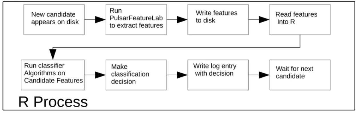
Develop a working on-line classifier system . . . 52
4 Results 54 Introduction . . . 54
Support Vector Machine Classifiers . . . 63 C5.0 Classifier . . . 66 Ensemble Classifiers . . . 70 5 Conclusions 79 Conclusions . . . 79 Implications . . . 80
Recommendations for Future Work . . . 80
Summary . . . 82
A R Packages and scripts 86 Common Script with No Preprocessing . . . 86
Script to train, test, and evaluate all of the models . . . 88
Script to train, test, and evaluate all of the models . . . 102
B Neural Network Plots, Raw Results and scripts 103 Plots . . . 103
Data . . . 108
C Support Vector Machine Results 120 Plots . . . 120
Data . . . 125
D C5.0 Results 137 Plots . . . 137
Data . . . 141
E Bagged Trees Results 152 Plots . . . 152
Data . . . 157
F Stacked Classifiers 165 Neural Network Ensemble Plots . . . 165
Neural Network Ensemble Data . . . 178
C5.0 Ensemble Plots . . . 190
G Pulsar Characteristics 209 Normal Pulsars . . . 209
Millisecond Pulsars . . . 210
More Exotic Pulsars . . . 211
Bibliography 212
Table
Page
4.1 Pulsar data sets . . . 55
4.2 Model Training Parameters . . . 57
4.3 Neural Network Models . . . 59
4.4 Neural Network Model Training Summary Statistics . . . 61
4.5 Support Vector Machine Models . . . 64
4.6 Support Vector Machine Training Summary Statistics . . . 66
4.7 C5.0 Models . . . 68
4.8 C5.0 Model Training Summary Statistics . . . 70
4.9 Recursive Partitioned Tree Model Training Summary Statistics . . . 72
4.10 Neural Network Models . . . 76
4.11 Neural Network Training Results, Base Models Built With Downsampling 77 4.12 C5.0 Ensemble Models . . . 77
4.13 C5.0 Classifier Training Statistics . . . 78
Figure
Page
1.1 Pulsar data collection process . . . 2 1.2 Dispersion from the Interstellar Medium. From D. Lorimer and Kramer(2005) . . . 4 1.3 Pulsar signal processing pipeline . . . 4 1.4 Diagnostic plot for Pulsar J0820-1350 . . . 5 1.5 Diagnostic plot of background noise in the direction of 0814-1341 . . . . 8 1.6 Diagnostic plot of radio frequency interference in the direction of 0723-1342 9 2.1 Nonlinear transformation Adapted from Scholkopf et al. (1997) . . . 25
2.2 Maximum Margin Hyperplane and Support Vectors Adapted from Burges (1998) 26
2.3 Results for linear and nonlinear models Adapted from Weston et al. (2000) . . . . 31
3.1 Classifier System . . . 53 4.1 Box and Whiskers plot with all three metrics returned from training the
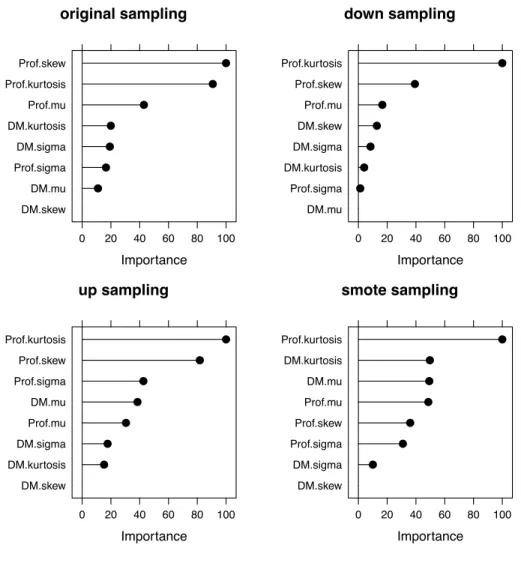
neural network models . . . 60 4.2 Neural network model variable importance plots for four di↵erent sampling
methods . . . 63 4.3 Neural network model variable importance plots for the ROSE sampling
method . . . 64 4.4 Box and Whiskers plot with all three metrics returned from training the
SVM models . . . 65 4.5 Support Vector Machine variable importance plots for four di↵erent
sam-pling methods . . . 67 4.6 Support Vector Machine variable importance plots for ROSE sampling
methods . . . 68 4.7 Box and Whiskers plot of the three metrics returned from training the
models . . . 69 4.8 C5.0 Model Variable Importance plots for four di↵erent sampling methods 71 4.9 Box and Whiskers plot of the three metrics returned from training the
models . . . 73 4.10 Bagged Tree Model Variable Importance plots for four di↵erent sampling
methods . . . 74 4.11 Bagged Tree Model Variable Importance plots for the ROSE sampling
method . . . 75 B.1 Neural network model variable dot plot . . . 104 B.2 Neural network model variable box and whiskers plot . . . 105 B.3 Neural network model variable importance plot for four sampling methods 106 B.4 Neural network model variable importance plot for ROSE sampling . . . 107 C.1 Support vector machine model variable dot plot . . . 121 C.2 Support vector machine model variable box and whiskers plot . . . 122 C.3 Support vector machine model variable importance plots for four sample
sets . . . 123 viii
C.4 Support vector machine model variable importance plots for ROSE sample
sets . . . 124
D.1 C5.0 model dot plot . . . 138
D.2 C5.0 model box and whiskers plot . . . 139
D.3 C5.0 model variable importance plots for four sample sets . . . 140
E.1 Bagged tree model dot plot . . . 153
E.2 Bagged tree model box and whiskers plot . . . 154
E.3 Bagged tree model variable importance plots for four sample sets . . . . 155
E.4 Bagged tree model variable importance plots for ROSE sample sets . . . 156
F.1 Neural network ensemble model dot plot . . . 166
F.2 Neural network ensemble model box and whiskers plot . . . 167
F.3 Neural network ensemble model variable importance plots for original sam-ple sets, 1 of 2 . . . 168
F.4 Neural network ensemble model variable importance plots for original sam-ple sets, 2 of 2 . . . 169
F.5 Neural network ensemble model variable importance plots for downsam-pled data, 1 of 2 . . . 170
F.6 Neural network ensemble model variable importance plots for downsam-pled data, 2 of 2 . . . 171
F.7 Neural network ensemble model variable importance plots for upsampled data, 1 of 2 . . . 172
F.8 Neural network ensemble model variable importance plots for upsampled data, 2 of 2 . . . 173
F.9 Neural network ensemble model variable importance plots for SMOTE sampling, 1 of 2 . . . 174
F.10 Neural network ensemble model variable importance plots for SMOTE sampling, 2 of 2 . . . 175
F.11 Neural network ensemble model variable importance plots for ROSE sam-pling, 1 of 2 . . . 176
F.12 Neural network ensemble model variable importance plots for ROSE sam-pling, 2 of 2 . . . 177
F.13 C5.0 ensemble model dot plot . . . 191
F.14 C5.0 ensemble model box and whiskers plot . . . 192
F.15 C5.0 ensemble model variable importance plots for original sample set . . 193
F.16 C5.0 ensemble model variable importance plots for downsampled data . . 194
F.17 C5.0 ensemble model variable importance plots for upsampled data . . . 195
F.18 C5.0 ensemble model variable importance plots for SMOTE sampling . . 196
F.19 C5.0 ensemble model variable importance plots for ROSE sampling . . . 197
G.1 TheP/ ˙P diagram (From D. Lorimer and Kramer (2005) . . . 210
Chapter 1
Introduction
Background
Pulsars are rapidly rotating neutron stars which emit a strong beam of energy through mechanisms that are not entirely clear to physicists. These very dense neu-tron stars are used by astrophysicists to study many phenomena. Fundamental tests of general relativity can be made using them as tools (D. Lorimer and Kramer, 2005). Currently, an experiment is being performed to try to detect gravitational waves by the North American Nanohertz Observatory for Gravitational Waves (2012) by study-ing the timstudy-ing variations of an array of pulsars scattered around the celestial sphere. These experiments in fundamental physics require a large set of pulsars for study, providing the impetus for systematically searching the sky for new pulsars. Pulsars discovered in ongoing pulsar surveys, as well as in the reprocessed data of several archival surveys, are continually being added to the census of pulsars in the nearby universe.
Problem Statement
Searching for pulsars is a very labor-intensive process, currently requiring skilled people to examine and interpret plots of data output by analysis programs. An automated system for screening the plots would speed up the search for pulsars by a very large factor. Research to date on using machine learning and pattern recognition has not yielded a satisfactory system. This work proposes to research, identify, and propose methods to overcome the barriers to such a system.
Figure 1.1: Pulsar data collection process
Analog to Digital Conversion
Streaming Fast
Fourier Transform Accumulate Write to Disk
Searching for Pulsars
Searching for pulsars is a compute-intensive and human-intensive task. The raw data is collected from a large (40 to 100 meter diameter) radio telescope at a very high sample rate with a specialized radio telescope receiver system and custom hardware signal processor. The signal processor receives the signal from the telescope, digitizes it, and performs a Fourier transform on the time series, changing it into a power spectrum with many frequency channels. Each channel represents the instantaneous signal power in a small frequency band 1 to 4 megahertz (MHz) wide. The instanta-neous power spectrum is sent to a computer where it is stored for later processing. Figure 1.1 shows a simplified schematic of the data collection process.
Once the time series of power spectral data is stored on disk, it can be processed to search for pulsars. Not only is the pulsar signal very faint and buried in random background noise, it is also often obscured with radio frequency interference (RFI). When many samples of a faint signal buried in random noise are averaged together, the signal-to-noise ratio is improved because the random noise cancels while the (non-random) signal builds up with the addition of each time sample (Hassan & Anwar, 2010). However, RFI is not a random process and does not average out over time, so the first step in the processing is to attempt to find and remove any RFI signals from the data to avoid confusing the RFI with an astronomical signal.
signal-to-noise ratio, in the case of pulsar search data processing, an added complication is that the pulse period is unknown, and so the averaging process must be performed at many di↵erent trial pulse periods (known as folding) to search the pulse period parameter space and find the true pulsar period.
Another parameter space that must be searched is the Dispersion Measure (DM) space. Dispersion is caused by the interstellar medium, and is di↵erent for every pulsar, depending on its distance and the number of electrons in the interstellar medium in the direction of the pulsar. Dispersion causes the lower frequencies of the signal to arrive later than the higher frequencies. This smears out, or disperses, the pulse. This smearing will completely obliterate the pulse if the signal is not de-dispersed before folding. Figure 1.2 shows the e↵ects of dispersion on the time of arrival of the pulse. Note that in the upper part of the figure, the signal in each frequency channel across the band is spread nearly evenly in time. The lower panel shows the results of de-dispersing the pulse and summing all of the frquency channels. The pulse is clearly visible with high signal to noise ratio.
The degree of dispersion given by the dispersion measure parameter must also be searched at the same time as the pulsar period, creating a combinatorial explosion in the number of output data sets created from each input data set. The output data sets are usually presented to the scientist graphically and these plots are called
diagnostic plots (described below). A simplified diagram of this signal processing pipeline is described in Figure 1.3. Complete details of the signal processing pipeline in typical use may be found in D. Lorimer and Kramer (2005) or in McLaughlin (2011).
The final step in the classical analysis of pulsar search data is the manual ex-amination of diagnostic plots like the one in Figure 1.4. The plots are examined
Figure 1.2: Dispersion from the Interstellar Medium. From D. Lorimer and Kramer (2005)
.
Figure 1.3: Pulsar signal processing pipeline Read from Disk Search for and
Excise RFI De-disperse the Data Search for Periodic Signals
Search for
Figure 1.4: Diagnostic plot for Pulsar J0820-1350
by astronomers or trained volunteers (often interested high school or undergraduate students!) to determine if a pulsar signal is likely present in the data. Diagnostic plots that appear to contain a pulsar signal are saved, and that region of the sky is observed again to confirm whether a pulsar is present. For a particular pointing on the sky, a few hundred or a thousand diagnostic plots might be created, resulting in millions of plots being created from a large-scale survey.
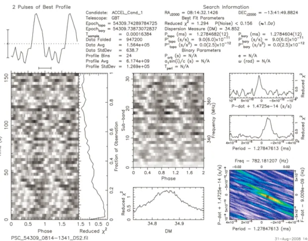
Figures 1.4 – 1.6 show diagnostic plots derived from Green Bank Telescope 350 MHz data collected for the Pulsar Search Collaboratory (Heatherly, 2013) (Adapted with permission). Figure 1.4 shows the plot for known pulsar J0820-1350. Data shown in tabular form in the upper right corner of the plot give the summary of the
statistics of the processed data. An important measure is the value of Reduced 2,
It is important to note that the Reduced 2 value builds over time as the data are
processed and compared to the model. This can be seen in the Reduced 2 vs Time
subplot (Labeled “C” in Figure 1.4).
There are four main features in the plots that astronomers use when deciding if a candidate could be a pulsar:
• First, in the 2 Pulses of Best Profile subplot in the upper left-hand corner of the figure, labeled “A”, the peaks should be significantly above the noise floor. Compare the error bars in the lower left corner of the same subplot in Figures 1.4 and 1.5.
• Second, in thePhase vs Time subplot, labeled “B”, vertical lines in phase with the peaks should appear throughout the entire observation time, unless, as in this case, the telescope beam is drifting across the sky, in which case the pulsar should smoothly come into the beam and drift out later. This indicates that the signal is continuous in time, as pulsar signals usually are. In this plot, the pulsar drifted into the beam at the beginning of the pointing, and then was constant throughout the rest of the pointing. The data file that follows this one in time would show the pulsar strongly in the beginning of the scan, and show it drifting out of the beam at the end of the scan.
• Third, in thePhase vs Frequency subplot, labeled “E”, the vertical lines should also span most of the frequency space, indicating the signal is a broadband signal, which is characteristic of a pulsar signal. Compare this with Figure 1.6, a plot of a man-made interference signal, where the signal is present only at a narrow band of frequencies.
• Fourth, a bell-shaped curve in the DM vs Reduced 2 subplot, labeled “D”,
shows that the signal’s reduced 2 value depends strongly on DM, peaking at
the trial DM, as it should. Compare this with the plot in Figures 1.5 and 1.6, where there is no strong dependence of Reduced 2 with DM.
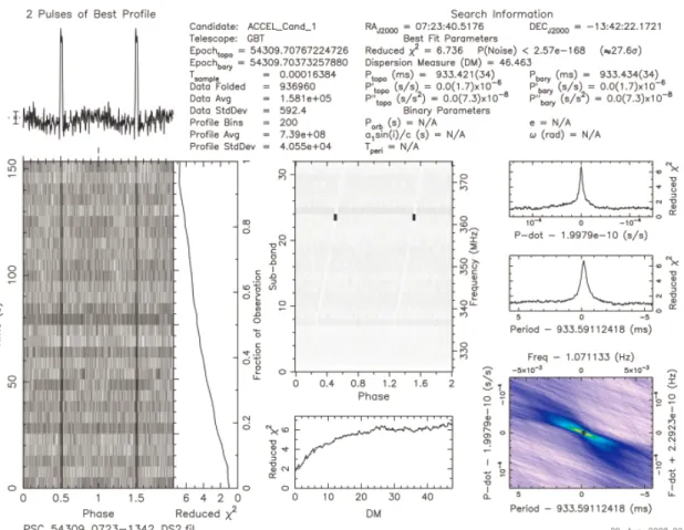
Figure 1.5 shows a plot generated from a signal that is normal background noise. Note the lack of systematic signals that were present in Figure 1.4. The error bars on the2 Pulses of Best Profile subplot are nearly as large as the pulse peaks. ThePhase vs Time and Phase vs Frequency subplots are disorganized and appear random. The
DM vs reduced 2 subplot shows only a very weak dependency of 2 on DM.
Figure 1.6 shows a plot generated from a man-made interference signal. Some of the charateristics seem to be the same as the pulsar signal in Figure 1.4. However, other characteristics are clearly di↵erent. The Phase vs Frequency subplot shows a strong signal at only a small band of frequencies, rather than across the band as might be expected of a true pulsar signal. TheDM vs Reduced 2 subplot shows no
Figure 1.5: Diagnostic plot of background noise in the direction of 0814-1341
Research Goal
The first published attempt to use a machine learning approach to detect pulsars in diagnostic data was published by Eatough et al. (2010). Their work used 14,400 pointings out of the Parkes Multibeam Pulsar Survey (PMPS), one of the largest comprehensive searches undertaken to date (Manchester et al., 2001). The 14,400 beams were processed through their standard pulsar search pipeline, generating 2.5 million candidate plots containing possibly all types of pulsars: binary pulsars, slow pulsars, and millisecond pulsars. Out of these 2.5 million plots, 501 pulsars were found by manual means, yielding a very small 501
2,500,000 = 0.02% success ratio. Such a
Figure 1.6: Diagnostic plot of radio frequency interference in the direction of 0723-1342
error-prone.
An automated method of screening the candidates is needed to reduce the human e↵ort needed to examine the candidate plots. Eatough et al. (2010) used an Artificial Neural Network (ANN) as a binary classifier to screen the 2.5 million candidate plots. The goal of the proposed research was to develop an improved method for pulsar identification using supervised machine learning techniques. Private communications with pulsar scientists (Demorest, 2013; Ransom, 2013) set the goals as
• The false positive rate should be less than 5%.
state of the art.
• Recall greater than 99% (Less than 1% of the pulsars are missed)
These are very difficult specifications to meet, but the relaxed false positive rate specification from that achieved by Eatough et al. (2010) provided a ray of hope. In fact, a paper (Morello et al., 2014) reports that they have acheived a 100 percent recall and just 0.64 percent false positive rate on a large data set. See Chapter 2 for more on this paper. Additionally, a recent paper by Lyon, Stappers, Cooper, Brooke, and Knowles (2016) provides more analysis and a mathematical background for choosing features.
Prior Research and Significance
As noted in the background section, there are more and larger pulsar surveys being planned for current and future telescopes. The Five Hundred Meter Spherical Telescope being built in China will be able to find as many as 5,000 pulsars in a short amount of time (Smits, Lorimer, et al., 2009). The Square Kilometer Array (SKA) is expected to find more than 20,000 pulsars (about 10 times the number currently known!) (Smits, Kramer, et al., 2009). As the ratio of candidates to confirmed pul-sars is about 10,000:1, upwards of 200 million candidates will need to be examined to complete the SKA survey. Clearly, it is impractical to examine all 200 million candidates with human eyes.
Research in automated pulsar search is in its infancy. Research in machine learn-ing for buildlearn-ing classifiers is a mature area. One characteristic of the pulsar search problem that makes this research interesting is the imbalanced training data avail-able. The very small number of known pulsars and the large amount of data available means that the training must be done with a very imbalanced data set, or else large
amounts of data without pulsars must be discarded. Other machine learning tech-niques have not been used in identifying pulsars thus far, and it is worthwhile to consider some of these techniques. One such technique is the Support Vector Ma-chine. The SVM can perform well in cases where there is an imbalance in the classes available in the training data, since only training examples nearest the maximum-margin hyperplane separating the two classes are required. Sei↵ert, Khoshgoftaar, Van Hulse, and Napolitano (2007) discusses the issues involved with classifying very rare events using the SVM.
Experience with many large-scale pulsar surveys (Eatough et al., 2010; D. R. Lorimer, 2011) has shown the need for a more automated system for classifying pulsar candidates. Eatough et al. (2010) proposed an ANN utilizing eight input features derived from plots generated by the pulsar search software output. This ANN, when trained, reduced the number of candidates that had to be viewed from 2.5 million to 13,000. Unfortunately, it detected only about 92% of the pulsars in the test data set. Changing the scoring added to the number of false positives but did not materially increase the success rate. An attempt to improve on these results was recently published (Bates et al., 2012), but the e↵ort failed in spite of using 14 more parameters in the ANN inputs. This lack of success with more features suggests that the features chosen for the studies by Eatough et al. (2010) and Bates et al. (2012) may have not been the best features to use for classification, leading to failure of the trained network to generalize well. Studies of optimizing the feature sets used in classification problems have been done (Van Hulse, Khoshgoftaar, Napolitano, & Wald, 2009), and algorithms have been developed to automate the feature optimization. Weston et al. (2000) outlines a procedure for choosing features to be used in support vector machine classifiers. Since an ANN is a special case of a support vector machine (Vapnik, 1999),
these techniques may be applied to the problem.
The work of both Eatough et al. (2010) and Bates et al. (2012) used simple statis-tics derived from the pulsar candidate plots as inputs to the ANN. These statisstatis-tics may not include critical information that was lost when the plots were reduced to simple statistics. In addition, millisecond pulsars, a class of pulsars especially prized for their stable spin periods and emissions, are underrepresented in the training data they used in training their ANN. Both of these problems need to be studied further as part of this work.
Eatough comments that the CPU time to run the ANN is a very small fraction of the time spent creating the candidate plot in the first place (2 minutes vs. 3 hours). From that perspective, it is feasible to cascade several classifiers together to extract more pulsars from the stream and exclude more false positives. Again, for this application it is important to minimize false negative results.
In addition to the ANN research described above, work has been done on improv-ing the algorithms for scorimprov-ing the candidate plots. Usimprov-ing these improved techniques, Keith et al. (2009) found 28 more pulsars in a data set that had already been mined. Their method included performing statistical analyses on the data making up the diagnostic plots. They analyzed thesubband, DM curve, and pulse profile plots, and combined the output scores from these analyses to form a score to decide whether a candidate was a strong candidate.
A very recent system called PEACE: Pulsar Evaluation Algorithm for Candidate Extraction (Lee et al., 2013) demonstrated the utility of careful feature selection in an algorithm similar to the one described above. This paper used six quality factors
in the scoring of the pulsar candidate. They achieved good results using these six factors, with 100% of the known pulsars in the data set ranked in the top 3.7% of the
candidates. These experiences will be used to help define the candidate feature sets to be optimized.
An e↵ort was made by Lyon et al. (2016) to rigorously derive a feature set from the data provided by (Morello et al., 2014). That feature set is used for the experiments in this research.
Other Machine Learning Methods
If one subscribes to the No Free Lunch theorems (D. Wolpert & Macready, 1997), then one should try to use the a priori knowledge of the problem to choose the best possible algorithm match to the problem. Support vector machines will be investigated to find out if they o↵er advantages over the ANN, and to provide a structure for investigating the feature set to be used.
Naive Bayes classifiers were investigated as part of the background work for this paper but do not seem to be applicable to this work due to the difficulty of establishing prior probabilities due to the rarity of the pulsars in the data.
Machine Learning in the face of unbalanced training data
Work by Sei↵ert et al. (2007) on very imbalanced data sets shows that even with the minority making up as little as 0.1% of the examples, e↵ective classifiers can be built using techniques to mitigate the e↵ects of the unbalanced data set. Their work used 11 di↵erent learning algorithms and built over 200,000 classifiers. Their conclusions show that data sampling, a technique for selecting a subset of data for learning purposes, can increase the performance of the classifiers.
Barriers and Issues
Automated pulsar searching is a difficult problem due to the relative scarcity of exemplars and the huge volumes of sometimes poor-quality data. Pulsar signals also
exhibit a great deal of variability from pulsar to pulsar. Some produce very narrow pulses, while others produce wide pulses. The pulsar signal, even in the best of cases, is weak and buried in noise. Combined with terrestrial interference, the signals are very difficult to find even for human eyes. In addition, machine learning is a very new topic in the pulsar search community. Only a few papers have been published on the subject (Bates et al., 2012; Eatough et al., 2010; Morello et al., 2014). Although there is other on-going research by astronomers, there are no computer science researchers involved in these studies.
Finally, the data sets themselves are many tens to hundreds of terabytes in size. Even with permission to use the data, it is unwieldy to copy it around the internet. Fortunately, astronomers are willing to help by physically copying the data onto media and shipping it to one another once it is public.
Unbalanced Training Data
One particularly difficult problem involves the data available to train a machine learning algorithm. For example, in Eatough et al. (2010), only 259 pulsars and 1625 non-pulsar signals were available for training. This was culled out of a total of 2,500,000 diagnostic plots. Particularly scarce in the training data are the millisecond pulsars. These have some characteristics that di↵er from normal pulsars that caused them to be missed in larger proportion than the normal pulsars in the ANN stud-ies. Some ideas to counter this problem are to use some of the ideas of Hu, Liang, Ma, and He (2009) and Sei↵ert, Khoshgoftaar, Van Hulse, and Napolitano (2009) in synthesizing and augmenting the minority exemplars. This is an opportunity for research as much as it is a barrier!
New Area of Research
As the application of machine learning techniques is new to the field of pulsar astronomy, there has not been much research published to guide the way forward. There is enthusiasm in the pulsar astronomy community for these techniques, and a great deal of data is publicly or semi-publicly available for experimentation, but there are many data formats and di↵ering data quality across the di↵erent data sets.
Definition of Terms
Binary pulsar A pulsar in orbit around a companion star, or vice versa.
Dispersion The e↵ect on a broadband electromagnetic signal traveling through the interstellar medium that imparts a frequency dependent delay to the signal.
Dispersion Measure A measurement of the delay experienced by the pulsar signal as it transits the interstellar medium. It is a↵ected by the electron density along the line of sight. The units of dispersion measure are parsecs per cubic centimeter.
Folding Averaging a time series signal using a particular repetition period
Interstellar Medium The gases and ions between stars. Space is not quite a vac-uum.
Millisecond Pulsar A pulsar with a period measured in milliseconds.
Pulsar A rapidly rotating neutron star that emits a powerful beam of energy as it rotates
Power Spectrum A measurement of the signal power as a function of frequency
Radio Frequency Interference Unwanted signals generated by humans or natural processes that interfere with reception of desired signals
Reduced 2 The measure of how a signal di↵ers from an assumed model, which in
the case of radio astronomy data is white gaussian noise.
Slow pulsar A pulsar with a period approaching or exceeding 1 second.
Summary
Pulsars are rapidly rotating neutron stars which emit a strong beam of energy through mechanisms that are not entirely clear to physicists. These very dense stars are used by astrophysicists to study many basic physical phenomena, such as the behavior of plasmas in extremely dense environments, behavior of pulsar-black hole pairs, and other extreme physics. Many of these tasks require a large ensemble of pulsars to provide enough information to complete the science.
In order to provide more pulsars to study, there are several large-scale pulsar sur-veys underway, which are generating a huge backlog of unprocessed data. Searching for pulsars is a very labor-intensive process, currently requiring skilled people to ex-amine and interpret plots of data output by analysis programs. An automated system for screening the plots would speed up the search for pulsars by a very large factor. Eatough et al. (2010) recounts a private communication (Lee) describing an auto-mated pulsar candidate ranking algorithm. A method of using scores that indicate the degree of similarity between the candidate and a typical pulsar is described in another paper (Keith et al., 2009). Neither of these last two methods used ANNs or other machine learning techniques to inspect plots, rather the algorithms were used as a filter to limit the number of candidate plots that needed to be viewed.
The approach of using artificial neural networks is significant since it may allow an automated detection and classification pipeline to be used to relieve the burgeoning backlog of pulsar search data and to allow economical reprocessing of archived search data. Reprocessing of data is desirable when advances in search algorithms raise the possibility of additional pulsars being found in the archived data. Some of the most sought-after and rare pulsars are those found in binary systems, where the pulsar is orbiting another object, or where two pulsars are orbiting each other. These binary pulsars require advanced search algorithms that take into account the acceleration of the pulsars due to the presence of its orbiting companion. Before recent increases in the available computing power available to researchers, these advanced algorithms were not typically run on all data due to the extra computational complexity. Older data sets may yield some of these exotic systems if the data are reprocessed with new algorithms including automated detection and classification methods.
Research to date on using machine learning and pattern recognition has not yielded a satisfactory system, with more than 7% of the pulsars in a test data set missed by the first automated system to attempt this problem. Later systems have claimed 100% recall, but this needs further research to confirm. This work proposes to research, identify, and propose methods to overcome the barriers to building an improved classification system with a false positive rate of less than 0.5% and a recall of near 100%.
Chapter 2
Review of the Literature
Machine Learning in Astronomy
Machine learning algorithms were not applied in pulsar searching prior to Eatough et al. (2010). They have been used in other branches of astronomy in such applica-tions as the classification of galaxies (Lahav, Naim, Sodr´e, & Storrie-Lombardi, 1996; Zhang, Li, & Zhao, 2009), in estimation of redshifts of stars in the Sloan Digital Sky Survey (Firth, Lahav, & Somerville, 2003), and in the classification of microlensing events from large variability studies (Belokurov, Evans, & Du, 2003).
One of the new topics in astronomy is transient detection. Transient objects appear in astronomical images from many causes. Some are asteroids, comets, and other near-earth phenomena, while others are more exotic, such as Gamma-ray bursts (GRB), supernovae, and variable stars. New telescopes are being built to image the sky rapidly, so that transients can be detected quickly, giving other telescopes time to follow up on them before they fad away. A prime example of this is the work by Morgan et al. (2012) in applying machine learning to classify GRBs as coming from sources with a particularly interesting redshift. The purpose is to maximize use of the avaiable follow-up time to study these more interesting GRBs. This work uses a Random Forest set of classifiers to do the work. Another work using the Random Forest approach is from Brink et al. (2013) that is used to look for real transient events from the Palomar Transient Factory, a telescope dedicated to looking for transient events. This system correctly classifies 92% of real transients in the data, with a 1% false positive rate. For transient detection in the Pan-STARRS1 Medium Deep Survey, a machine learning system has been applied to the problem, yielding a 90%
recall rate with a 1% false positive rate (Wright et al., 2015).
Machine Learning in Pulsar Search
Eatough et al. (2010) used an Artificial Neural Network (ANN) as a binary classi-fier to screen the 2.5 million candidate plots. The e↵ort used a set of 8 input features derived from candidate plots as the input vector to the ANN. In addition to these 8 features, an additional small trial was done with a set of 12 features with minimal e↵ect on the success rates. The following are the features extracted from the data forming the diagnostic plots and used in the feature vector (the last 4 features listed were not used in the full experiment):
• Pulse profile signal-to-noise ratio (SNR)
• Pulse profile width
• 2 of the fit to the theoretical dispersion measure (DM) - SNR curve • Number of DM trials with SNR> 10
• 2 of the fit to the optimized theoretical dispersion measure (DM) - SNR curve • 2 of the fit to the theoretical acceleration - SNR curve
• number of acceleration trials with SNR >10
• 2 of the fit to the optimized theoretical acceleration - SNR curve • RMS scatter in subband maxima
• Linear correlation across subbands
• RMS scatter in subintegration maxima
From the data, which contained 501 pulsars, training data consisting of 259 input vectors from known pulsars and 1625 input vectors from non-pulsar signals were used to train the ANN. An additional validation data set was reserved from the data set with 28 pulsar signals and 899 non-pulsar signals. The remainder of the data, which contained the rest of the pulsars, was used as a test sample. Unfortunately, some of the test sample contained pulsars that were used in training, which makes some of the statistics a bit optimistic.
This ANN was very e↵ective in reducing the number of plots to be examined by eye from 2.5 million to 13,000, a reduction of a factor of almost 200. However, the ANN recovered only about 92% of the known pulsars in the data set, which is not acceptable to scientists (Ransom, 2013), who would demand a false negative rate of at worst a few percent before entrusting the search to the machine.
Bates et al. (2012) also attempted to use this method to find pulsars, but were not as successful as Eatough et al. (2010). They used 22 features in the input vector, including all of the features used by Eatough et al. (2010). Their success rate was no better with more features. This lack of success with more features suggests that Eatough et al. (2010) and Bates et al. (2012) may have not chosen the features to use for classification in an optimal way, leading to failure of the trained network to generalize well.
Recently, a system called SPINN (Morello et al., 2014) was developed that can detect 100 percent of the known pulsars in the High Time Resolution Universe sur-vey (Keith, 2013). This system uses a custom neural network software implementa-tion that allows finer control of the learning process than that used by Eatough et al. (2010). To improve learning and generalization the system employed recommenda-tions from earlier work on efficient backpropagation algorithms by LeCun, Bottou,
Orr, and Muller (1998). Specifically, the following recommendations were employed:
• Feature scaling to to ensure each feature has zero mean and unit standard deviation over the traning set.
• The hyperbolic tangent function as an activation function
• Training of the system in batches containing di↵erent mixes of training data. In addition to these techniques, the class imbalance was mitigated by oversampling the minority class pulsars so that the ratio of pulsars to non-pulsars was 4:1. This may potentially be a problem! It’s not clear that in the 5-fold cross validation that they took care to not have the oversampled pulsar candidates in the test and training sets...
The feature set used in this research was smaller than that used by Eatough et al. (2010) and Bates et al. (2012), lending credence to the speculation that better feature selection could have improved performance of the e↵orts. The specific features used here are:
• Signal to Noise of the folded pulse profile
• Intrinsic equivalent duty cycle of the pulse profile
• Ratio between the period and dispersion measure
• Validity of the optimized dispersion measure
• Time domain persistence of the signal
• Root-mean-square distance between the folded profila and the sub-integrations that make up the profile
It should be noted that one of the criteria mentioned in the description of Fig-ure 1.6 as being critical to human classification is not used in this featFig-ure set. The authors state that using continuity of the Phase vs Frequency plots hurt the perfor-mance. However, In other surveys with strong narrowband interference, this may be a very good feature to use to identify RFI.
Studies on optimizing the feature sets used in classification problems have been done (Van Hulse et al., 2009), and algorithms have been developed to automate the feature optimization. Weston et al. (2000) outlines a procedure for choosing features to be used in support vector machine classifiers. Since an ANN is a special case of a support vector machine (Vapnik, 1999), these techniques may be applied to the problem. Many of the papers cited in the section above on transient science machine learning algorithms spend a great deal of time on feature selection.
Lyon et al. (2016) have released work on optimal feature selection for the pulsar search problem. This work condenses the data in the pulsar data files into eight features:
• Mean of the integrated profileP.
• Standard deviation of the integrated profile P.
• Excess kurtosis of the integrated profile P.
• Skewness of the integrated profileP.
• Mean of the DM-SNR curveD.
• Standard deviation of the DM-SNR curveD.
• Skewness of the DM-SNR curveD.
The work of all of these authors(Lyon et al. (2016), Eatough et al. (2010) and Bates et al. (2012)) used simple statistics derived from the pulsar candidate plots as inputs to the ANN. These statistics may not include critical information that was lost when the plots were reduced to simple statistics. In addition, millisecond pulsars, a class of pulsars especially prized for their stable spin periods and emissions, are underrepresented in the training data they used in training their ANN. Both of these problems need to be studied further as part of this work.
Eatough comments that the CPU time to run the ANN is a very small fraction of the time spent creating the candidate plot in the first place (2 minutes vs. 3 hours). From that perspective, it is feasible to cascade several classifiers together to extract more pulsars from the stream and exclude more false positives. Again, for this application it is important to minimize false negative results.
Zhu et al. (2014) have worked on the pulsar classification problem in a di↵erent way, by training a system to directly read the pulsar diagnostic plots. This sys-tem combines many techniques together to optimize the classification problem. The subplots identified in Figure 1.4 are fed to classifiers that classify the subplot as con-taining a pulsar or non-pulsar, and then in turn the output of these classifiers are fed into a second classifier that determines, based on the scores from the first classifier, if the sample is a pulsar or non-pulsar. This system has been tested on Green Bank Telescope data, and has given good results, with 100% of the pulsars scoring in the top 1% of the candidates. This yields about a 100 fold reduction in the number of candidates to be examined.
In addition to the ANN research described above, work has been done on improv-ing the algorithms for scorimprov-ing the candidate plots. Usimprov-ing these improved techniques,
Keith et al. (2009) found 28 more pulsars in a data set that had already been mined. Their method included performing statistical analyses on the data making up the diagnostic plots. They analyzed thesubband, DM curve, and pulse profile plots, and combined the output scores from these analyses to form a score to decide whether a candidate was a strong candidate.
A recent system called PEACE: Pulsar Evaluation Algorithm for Candidate Ex-traction (Lee et al., 2013) demonstrated the utility of careful feature selection in an algorithm similar to the one described above. This paper used six quality factors
in the scoring of the pulsar candidate. They achieved good results using these six factors, with 100% of the known pulsars in the data set ranked in the top 3.7% of the candidates. The features used by PEACE are:
• Signal to noise ratio of the folded pulse profile
• Topocentric period
• Width of the pulse profile
• Persistence of signal in the time domain
• Persistence of signal in the frequency domain
• Ratio between puslse witdth and Dispersion Measure smearing time
Support Vector Machines
Support vector machines (SVMs) are finding greater applications in data mining of large data sets, and in particular with pattern matching applications (Burges, 1998). Although support vector machines were developed starting in the 1970s (Han, Kamber, & Pei, 2011), they began to be studied in earnest in the 1990s (Cortes & Vapnik, 1995).
Figure 2.1: Nonlinear transformationAdapted from Scholkopf et al. (1997)
Support vector machines are machine learning algorithms that can extend linear modeling to nonlinear class boundaries. This is accomplished by transforming the inputs to the machine using a nonlinear function mapping (Witten, Frank, & Hall, 2011). For instance, a circular region could be transformed using a polar to rectan-gular mapping, thereby linearizing the problem, as shown in Figure 2.1 adapted from Scholkopf et al. (1997).
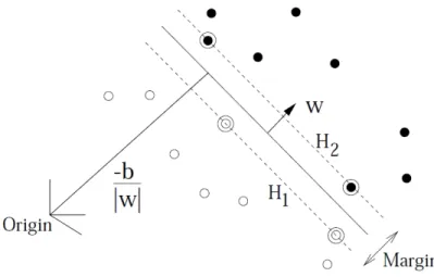
The basic idea of the support vector machine is to create a maximum-margin hyperplane between the classes, as shown in Figure 2.2. The maximum-margin hy-perplane is that hyhy-perplane that creates the greatest distance between the classes. The class instances that are closest to the maximum-margin hyperplane are called thesupport vectors (circled in Figure 2.2). The set of support vectors (tuples of data) define the hyperplane. None of the tuples further from the hyperplane matter to the SVM. This is important in the case of large data sets with a small number of minority classes, as only those tuples along the maximum-margin hyperplane are needed to define the classification.
Vapnik (1999) describes some of the useful theoretical properties of the SVM:
Figure 2.2: Maximum Margin Hyperplane and Support VectorsAdapted from Burges (1998)
• The learning process for constructing an SVM is faster than for a neural network
• While learning the decision rules, the support vectors are determined
• Changing the decision function is possible by changing only the kernel function used to define the feature space
The SVM is inherently a binary classifier. In the case of multiple possible classi-fications, an SVM for each possible decision must be created. An ensemble of SVMs and other classifiers may be profitably used to increase the classification accuracy of a given data set (Witten et al., 2011).
Statistical learning theory
The definition of the learning problem solved using the SVM comes from the statis-tical learning theory described by Vapnik (1999). The statisistatis-tical learning problem is defined in terms of minimizing the loss from misclassified observed data. The problem of pattern recognition (classification) is one of three problems described by Vapnik (1999). In the interest of brevity, the other two problems, regression estimation and density estimation, are not included in this treatment.
The model learning problem consists of three parts:
• A data generator that returns vectors taken from a fixed distributionP(x)
• A “supervisor” that returns an output vector for each of the input vectors.
• A learning machine capable of implementing a set of functions f(x,↵),↵2⇤. Choosing the bestf(x,↵),↵ 2⇤that maps the input to the output is the learning problem. The training data is a set of l independent identically distributed observa-tions taken from P(x, y) =P(x)P(y|x):
(x1, y1), . . . ,(xl, yl) (2.1)
Given these definitions, the learning problem is defined as minimizing the loss due to improper classification of the observations by the learned response of the machine. The expected value of the risk is given by the following equation, known as the risk functional:
R(↵) = Z
L(y, f(x,↵))dP(x, y) (2.2)
The goal of the learning process is to find the function f(x,↵) that minimizes equa-tion 2.2. Since the problem set addressed in this paper is one of pattern recogniequa-tion rather than regression or density estimation, the supervisor function simply outputs either a 0 or a 1, based on its evaluation of the indicator functions f(x,↵),↵2⇤. If the loss function is
L(y, f(x,↵)) = 8 > < > : 0 :y=f(x,↵) 1 :y6=f(x,↵) 9 > = > ; (2.3)
then evaluating the the risk functional given by equation 2.2 returns the probability of classification error. The learning problem in the pattern recognition case consists of
minimizing the probability of classification errors, based on minimizing equation 2.2 with the given training data as inputs.
Feature Selection in SVMs
Selecting which features of a data set to use in the classification process is an important consideration. Selection of features is done to eliminate redundant or irrelevant features from inclusion in the SVM. Careful selection of a subset of features can improve the classification capability of the SVM while reducing computational load. (Weston et al., 2000)
Importance of feature selection Feature selection in SVMs is important to im-prove the performance of the SVM. The performance of the SVM can be considered in two di↵erent ways. First, the speed of running the algorithm on training data and input data is a↵ected by the number of features used in the SVM. Second, the classification and generalization performance is negatively a↵ected by the inclusion of irrelevant or redundant features.
Feature selection algorithms and methods The feature selection problem may be formulated in two di↵erent ways:
• Given a set of features of a cardinalityn, and fixed subset of features of cardi-nality m, where m << n, find the m features that give the smallest expected errors.
• Given a maximum allowable expected error, find the smallestm that gives this expected error.
The expected error in either case is based on equation 2.3, with the input data modified to exclude some of the features by multiplying the input data by a vector
consisting of 0 where the feature is excluded, and 1 where the feature is included. Equation 2.4 shows the formulation of the problem. The task is to find and ↵ that minimize the modified loss functional.
⌧(⇢,↵) = Z
V(y, f((x⇤ ),↵))dP(x, y) (2.4) subject to the conditionsk k=m, where P(x, y) is fixed, but unknown, x⇤ is an element wise product of the input vector and the feature selection vector, V(...) is the loss functional, and k k0 is the 0 norm of the vector .
Two ways to attack this problem are known as the filter method and the wrapper method. The filter method is implemented by preprocessing the data to remove features before the SVM is trained, while the wrapper method provides the subset of features by repeatedly training the SVM with di↵erent feature sets and estimating the accuracy. This is a more computationally expensive procedure, but can give better results, since the power of the SVM is used to help sort out the feature set. This is still an active area of research, and much has been written on the subject of feature selection. Three promising approaches are given next.
Feature Selection in SVMs: R2W2 method Weston et al. (2000) introduce
a method that combines the filter method and the wrapper method in a way that eliminates the computational complexity of the wrapper method while preserving the superior results usually obtained. TheR2W2 algorithm consists of defining the SVM
problem in terms of the dual formulation expressed as the Lagrangian of the problem (as explained in chapter 7 of Hamel (2011)).
The paper defines the radius of the hypersphere,R containing the support vectors in feature space, and the margin, M, and from Theorem 1 in Weston et al. (2000),
the expectation of the error probability is given by E{Perr} 1 lE ⇢ R2 M2 = 1 lE R 2W2(↵0) (2.5)
where the expectation is taken over a training set of size l.
Minimizing equation 2.5 requires a search over a space as large as the number of features, which is a combinatorially difficult problem when a large number of features are included. To make this problem more tractable, Weston et al. (2000) suggest substituting real-valued vector 2Rn for the the binary-valued vector 2 {0,1}n.
This allows the use of a gradient descent algorithm to find the optimum value using the derivatives of the criterion, which are given below from Weston et al. (2000):
@R2W2( ) @ k =R2( )@W 2(↵0, ) @ k +W2(↵0, )@R 2( ) @ k (2.6) and @R2( ) @ k =X i 0 i @K (Xi, Xi) @ k X i,j 0 i j0 @K (xi, xj) @ k (2.7) and @W2(↵0, ) @ k = X i,j ↵0i↵0jyiyj @K (xi, xj) @ k (2.8) In order to test the utility of this method, Weston et al. (2000) derived SVMs using this method, and also using three standard filter algorithms:
• Pearson Correlation Coefficients
• Fisher Criterion Score
• Kolmogorov-Smirnov test
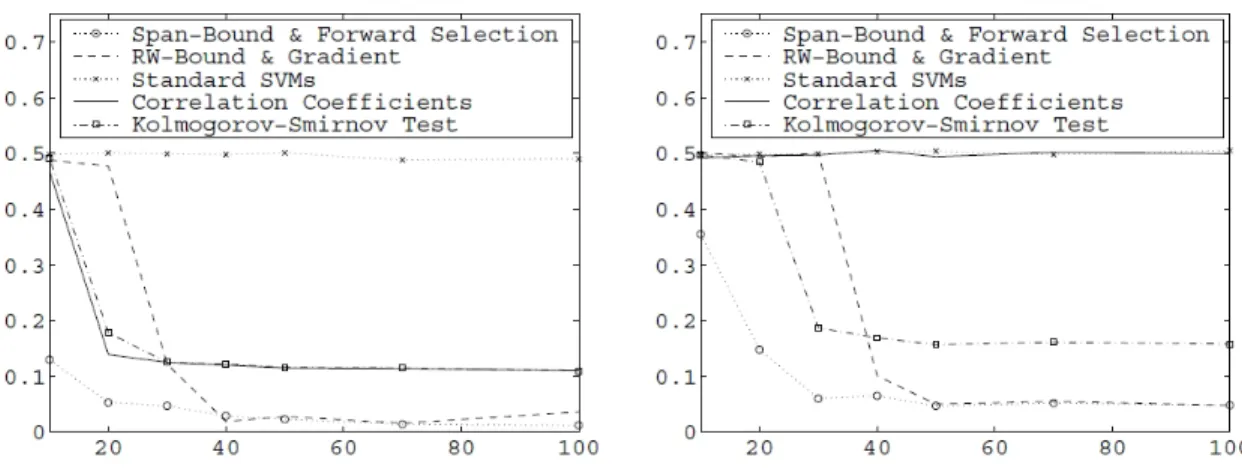
The data for this test was two synthetically derived data sets consisting of a linear problem and a nonlinear problem. The linear problem had six out of 202 dimensions
Figure 2.3: Results for linear and nonlinear models Adapted from Weston et al. (2000)
that were relevant, and even these were partially redundant. In the nonlinear problem, only two out of 52 dimensions were relevant.
The standard SVM algorithms performed poorly on this extremely redundant and irrelevant data set, even with a large number of training points. The best standard methods yielded an error rate of 13%, compared to 3% for this new method. Figure 2.3 shows the compilation of results for this experiment.
The algorithm was also tested on real-world data sets including a face recognition application and a cancer-screening application. In the case of the face recognition application, it outperformed the other methods of feature reduction, but the reduced feature set classifier did not perform any better than the full-rank classifier. For the cancer screening application, the algorithm did much better than the other feature reduction methods, and outperformed the full-rank classifier. Using all 7129 genes, the linear SVM made 1 error out of 34 test examples. The reduced feature set classifier of 20 genes built with the R2W2 classifier made no errors, while 3 errors were made
by a classifier built using the Fisher score. Classifiers using only 5 genes were also produced with theR2W2 method and the Fisher score method, and they made 1 and
While the toy problems were an extreme case of irrelevant data, the experiments showed that the introduction of irrelevant features into an SVM negatively a↵ects the classification ability of the machine, and so features should be screened to be sure that they are contributing to the information needed to properly classify the instances.
Genetic Algorithms for Feature Selection As mentioned previously, there are two di↵erent formulations of the feature selection problem. Either the number of features can be specified and the generalization error estimated, or the allowable gen-eralization error can be specified and the number of features needed can be estimated from the allowable error.
In the filter approach to the feature selection problem, a preprocessing step is used to separate the features to be used in the classification process from the features that are not used. This can be misleading to the classification algorithm, since the classification algorithm does not see all of the features, but only the subset that the preprocessing step did not remove.
In this study of feature selection, instead of using the standard k-fold validation routine, the genetic algorithm is used to estimate the error, based on including or excluding features in the calculation. This approach saves much of the computation that is required for a k-fold validation approach. This method can provide a lower variance, but a higher bias than cross-validation (Frohlich, Chapelle, & Scholkopf, 2003) The CHC genetic algorithm (Whitley, 1994) was used in this work. The defining feature of the CHC algorithm is the use of the population elitist strategy, where the best individuals of each generation replace the worst individuals of the parent generation. This allows faster mutations and hence a faster search strategy.
significant overfitting problem. The study also found that the leave-one-out error bounds can be used as an alternative performance measure. It usually provides a better generalization performance, but leads to more features being selected. Using the same R2W2 bound described earlier, along with the genetic algorithm, shows
a good generalization performance, comparable to the recursive feature elimination (RFE) method. The genetic algorithm is less computationally intensive, taking only about 1
3 the run time of the RFE algorithm for equivalent classification performance.
If the number of significant features is not known before beginning the analysis, the genetic algorithm method provides a more efficient method of determining the feature set to be used in the problem.
Optimal Feature Selection: Simultaneous training and feature selection
Nguyen and De la Torre (2010) provide a view on the problem that is di↵erent from the preceding treatments. This view is that there is value in working on both training and feature selection in one process. This is because, as noted above, doing the procedure in 2 steps can cause a loss of information. Other researchers have proposed this approach before, but their methods led to non-convex optimization problems. The approach of Nguyen and De la Torre (2010) propose a convex framework for jointly learning optimal feature weights and SVM parameters. The method provides a set of weights that are sparse, and therefore are useful for selecting features, with the missing weights corresponding to features that are trimmed.
The error function is modified for jointly learning the kernel and SVM parameters. Parameterizing the kernel and SVM parameters provides the mechanism to handle this learning method. The input space to feature space mapping is provided by a parameter vector, p, where (xi) = (xi, p). Di↵erent values of p provide di↵erent
nor-malized margins, describing the margin of the respective feature spaces in a way that can be compared between the two implementations are employed.
Class Imbalance
Work by Sei↵ert et al. (2007) on very imbalanced data sets shows that even with the minority making up as little as 0.1% of the examples, e↵ective classifiers can be built using techniques to mitigate the e↵ects of the unbalanced data set. Several sampling techniques are explored that have been used in the past to try to mitigate the e↵ects of the unbalanced class membership. The two most common techniques are random minority oversampling, (ROS) and random majority undersampling (RUS). In the former, the minority classes are duplicated randomly in the training data, while in the latter, some majority samples are randomly excluded from the training set.
Rather than randomly selecting majority members, techniques have been devel-oped to more systematically choose majority members to exclude, such as one-sided selection (Kubat and Matwin, 1997), where the majority samples to be discarded are determined to be redundant, or noisy in some way. Wilson’s Editing (Wilson, 1972) uses a kNN classification technique to evaluate which majority members get misclassified when classified against the remaining examples in the training set. The work of Sei↵ert et al. (2007) discussed above used 11 di↵erent learning algorithms and built over 200,000 classifiers. Their conclusions show that various methods of data sampling, a technique for selecting a subset of data for learning purposes, can increase the performance of the classifiers.
On the other side of the equation, another method of incrreasing the proportion of minority members is to manufacture synthetic samples by perturbing some of the features of the real members in a systematic way. This technique is known as
Synthetic Minority Oversampling Technique (SMOTE) (Chawla, Bowyer, Hall, and Kegelmeyer, 2002). The authors acknowledge that in classification problems, it is common for the number of examples of the normal case (the “uninteresting” case) to predominate by a large margin over the unusual or more interesting case, such as in our case of the pulsar vs non-pulsar. The paper shows that the combination of oversampling the minority class and undersampling the majority class can improve classifier performance of several di↵erent classification algorithms.
The methods of generating synthetic minority class members may work for the pulsar search problem since the physics that generate many of the signal properties are known, and new members of the pulsar class may be created by perturbing or modifying the existing class members within the physics from currently accepted pulsar models.
Ensemble Classifiers
Ensemble classifiers (Witten et al., 2011) have properties which may be surprising on first glance. Weak classifiers can be combined to produce strong classification results, in some cases stronger than atraining a model to a high degree of specializa-tion. This is due to the face that an ensemble of weak classifiers has more resilience than the highly trained single model. It has been suggested (Witten et al., 2011) that in many cases, experts are really quite ignorant! The process is similar to the appointment of a diverse committee of humans to help make a decision. Many times the committee members will bring a di↵erent perspective to the table and help the overall competence of the committee, even if they are not an expert in the field being discussed.
Three types of ensemble classifiers are common. Bagging is a technique where the output of several models is used in a non-weighted voting scheme to determine the
output of the group of models. Boosting (Schapire, 1990) is a similar technique, but the outputs of the various base classifiers are weighted in some way related to the strength of their classification of the sample. It is similar to the way a human will give more weight to a person’s opinion who is more learned in a subject.
A third way of combining multiple models isstacking, introduced by D. H. Wolpert (1992). Stacking is a way of combining models in a more intelligent way, using a meta-learner to combine the results of other learners, instead of using a simple voting mechanism, either weighted (boosting) or not weighted (bagging).
It is possible to combine several of the algorithms described in the previous sections to accomplish the classification task. An example of combining techniques is given by Sei↵ert et al. (2009). In this work, di↵erent types of resampling are combined with boosting to create classifiers that outperform more complex classifiers.
Chapter 3
Methodology
Methodology
The study concentrated on improving the classification performance of the work by Eatough et al. (2010) and Morello et al. (2014) by adding support vector machines and in experimenting with ensemble classifiers. Work in feature selection and in mitigating the imbalanced training data available for this problem was also shown to be very important. In particular, improving the false positive responses of the systems was of great interest to the pulsar community. The data set developed by Morello et al. (2014) as part of the SPINN work is from the Parkes Multibeam Pulsar Survey and is a superset of the data used by Eatough et al. (2010). This same data was used in the work by Lyon et al. (2016), to create their optimal feature set, and all of the data has been made public in the form used for the research by Lyon et al. (2016). This research continues use of this data set. The following general process was used as a guide for this research:
• Study the characteristics of normal and millisecond pulsars
• Develop a validation approach
• Study the information available for each pointing in the data
• Reproduce the results of the study by Lyon et al. (2016)
• Develop Support Vector Machine classifiers operating on the HTRU-1 data
• Design, prototype, train, test, and evaluate a system that can handle the HTRU-1 data set and improve upon the performance using the techniques described above
The remainder of this chapter details the methodology used to accomplish the above processes.
Study the characteristics of normal pulsars and millisecond pulsars
As a good hunter knows his quarry, learning the characteristics of di↵erent types of pulsars helps decide which algorithms are appropriate. It was theorized that di↵ er-ent types of pulsars might require di↵erent algorithms for best classification results. Results from previous research (Bates et al., 2012) show that millisecond pulsars have some characteristics, such as pulse width, di↵erent from common (normal) pulsars.
Develop a validation approach
The data sets available for research in pulsar search are necessarily sparse in the fraction of positive class examples. Given the imbalance in the data, it is difficult to develop a comprehensive validation and test data set. One way that this problem can be mitigated is to use multi-fold cross validation. This allows the training data to be used for testing during training by randomly selecting portions of the training data to use for training models, and holding out the rest of the training data for testing that particular model, The process is repeated using a di↵erent random selection of training data to train with, and di↵erent test data. Once the suite of models trained by the cross-validation technique were trained, they were tested with the pristine data that was held out from the training process, which in this case was 25% of the total HTRU-1 data set.
The requirements for pulsar classification were laid out in chapter 1. The most important criteria is that the pulsars should not be missed when candidates are run
through the classifier. But this must be balanced by the number of false positives generated. Obviously, a system that simply classified all samples as pulsars would meet the first criterion, but would be of no benefit. A secondary criterion is needed. The primary measure of the efficacy of the models generated in this reseach is
recall. The recall of the system is a measure of the number of positive samples that are lost by the system. It is defined as:
recall= T P
T P +F N (3.1)
In the field of diagnostic tests, recall is also called sensitivity. This measure was the primary selector for the training process. Other statistics were also calculated and used in the evaluation process. The specificity, which measures the proportion of negative examples correctly classified, is a marker for the false positive rate that was the secondary criterion. A low value of specificity will mean an excess number of false positives will be returned, diminishing the utility of the classifier. Specificity is defined as:
S = T N
T N +F P (3.2)
The FPR is the secondary measure of the e↵ectiveness of the classifier. It is defined as
F P R= F P
F P +T N (3.3)
The FPR can also be calculated from Specificity and Prevalence, where Prevalence is defined as:
P = (T P +F N)
T P +T N +F P +F N) (3.4)
So FPR may be calculated as