Spatial poverty traps?

wes lz;

POLIcy

RESEARCH WORKING PAPER

1862

Spatial Poverty Traps?

loakethe

difference between growth and contraction in living

Jyotsna

Jalan

Mlartin Ravallion :1denUical households?

Apparenty so. Evidence of spatal poverty traps

strengthens the case for

investtn in the geographic

capital of poor people.

The World Bank

Development Research Group

Public Disclosure Authorized

Public Disclosure Authorized

Public Disclosure Authorized

POLICY RESEARCH WORKING PAPER 1862

Summary findings

Can place of residence make the difference between with latent heterogeneity (whereby hidden factors entail growth and contraction in living standards for otherwise that seemingly identical households see different

identical households? consumption gains over time), yet identify the effects of

Jalan and Ravallion test for the existence of spatial stationary geographic variables.

poverty traps, using a micro model of consumption They estimate the model using farm-household panel growth incorporating geographic externalities, whereby data from post-reform rural China.

neighborhood endowments of physical and human They find strong evidence of spatial poverty traps. capital influence the productivity of a household's own Their results strengthen the case - both for efficiency capital. By allowing for nonstationary but unobserved and equity - for investing in the geographic capital of individual effects on growth rates, they are able to deal poor people.

This paper - a product of the Development Research Group - is part of a larger effort in the group to understand the

geographic determinants of poverty and the implications for policy. The study was funded by the Bank's Research Support Budget under the research project "Policies for Poor Areas" (RPO 681-39). Copies of the paper are available free from the World Bank, 1818 H Street NW, Washington, DC 20433. Please contact Patricia Sader, room MC3-632, telephone 202-473-3902, fax 202-522-1153, Internet address [email protected]. December1997. (32 pages)

The Policy Research Working .Paper Series disseminates the findings of work in progress to encourage the exchange of ideas about development issues. An objective of the series is to get the findings out quickly, even if the presentations are less than fully polished. The papers carry the names of the authors and should be cited accordingly. The findings, interpretations, and conclusions expressed in this paper are entirely those of the authors. They do not necessarily represent the view of the World Bank, its Executive Directors, or the countries they represent.

Spatial Poverty Traps?

Jyotsna Jalan and Martin Ravallion'

World Bank

Development Research Group, World Bank, 1818 H Street NW, Washington DC, 20433. The assistance and advice provided by staff of China's State Statistical Bureau-in Beijing and at

various provincial and county offices-are gratefully acknowledged. We thank Jaesun Noh of EVIEWS for technical support. Useful comments on the paper were received from seminar participants at the World Bank, University of Maryland, College Park, and at the MacArthur Foundation/World Bank Workshop on Emerging Issues in Development Economics, Washington DC, July 1997. The financial support of the World Bank's Research Committee (under RPO 678-69) is also gratefully acknowledged.

1 Introduction

Consider two households living in different areas but identical otherwise. Suppose that one of the areas is less well endowed with physical, human and social capital-in short geographic

capital-than the other. A spatial poverty trap can be said to exist if the household living in the

better endowed area sees its standard of living rising over time, while the other does not.

Various theoretical models have helped understand how such poverty traps can arise.2 _{If borne}

out by empirical evidence, spatial poverty traps suggest both efficiency and equity arguments for

investing in poor areas, such as by developing local infrastructure or by assisting labor export to better endowed areas.

Is it possible to test for spatial poverty traps? There are a number of problems.3

Aggregate growth empirics can test for divergence, whereby initially poorer areas grow at lower rates (following Barro and Sala-i-Martin, 1992). However, this is neither necessary nor

sufficient for a spatial poverty trap, since geographic aggregates do not allow one to separate effects which are external to individuals from purely internal effects (Ravallion and Jalan, 1996).

Suppose that one finds lower growth rates in areas with lower average wealth. This may reflect increasing returns to individual wealth, or geographic externalities, whereby living in a poor area lowers retums to individual investments. Aggregate geographic data cannot tell us which it is.

Instead, cross-sectional micro data might be used to test for geographic effects on living

2 On the theoretical possibilities for a poverty trap (with and without externalities) in a

neoclassical one-sector growth model see Azariadis (1996) and references therein.

standards at one point in time.4 However, to test for spatial poverty traps we need to identify dynamic effects, and to control for latent heterogeneity; that calls for longitudinal observations. Both household-level panel data and geographic data are clearly called for to have any hope of identifying spatial externalities in the growth process.

The problems do not end there. The geographic effects that one might find in household panel data may well be spurious in that they arise solely because geographic variables proxy for omitted non-geographic, but spatially autocorrelated, household characteristics. For example, we might find that the average wealth of an area is positively correlated with growth rates at

household level, controlling for individual wealth. But this may be because some household attribute relevant to growth, and positively correlated with average wealth, has been omitted. (Better own education may yield higher growth rates, be correlated with wealth, and be spatially autocorrelated. Then average wealth in the area of residence could just be proxying for

individual education.) One might attempt to deal with this by adding variables. But one might reasonably expect considemble latent heterogeneity in any micro data. Nor is it sufficient to allow for latent fixed effects in the levels of consumption (as is common practice). We need an econometric model which allows for individual effects in consumption growth rates.

At this point one might turn to the standard practice in panel data models of treating the latent heterogeneity as a time-invariant fixed effect (albeit a fixed effect in the growth rates, rather than the levels of consumption). However, this immediately wipes out any hope of identifying impacts of the time-invariant geographic variables of interest-of which there are

4 See, for example, Borjas (1995) on neighborhood effects on schooling and wages in the U.S.,

likely to be many. In that case, the cure to the problem of latent heterogeneity leaves an

econometric model which is unable to answer many of the questions we started out with. Nor,

for that matter, is it obviously plausible that the heterogeneity in individual effects on growth

rates would in fact be time invariant; common macroeconomic and geo-climatic conditions

might well entail that the individual effects vary from year to year.

This paper proposes an estimable microeconometric model of consumption growth which

can identify underlying (including time-invariant) geographic effects while at the same time

allowing for latent heterogeneity in household-level growth rates. We are able to test whether consumption growth rates at the farm-household level vary spatially after controlling for both

observed and unobserved heterogeneity at the household level.

Our theoretical model extends the Cass-Koopmans-Ramsey model of optimal consumption growth in a straightforward way to allow geographic effects on the marginal product of own capital, analogous to the role of knowledge externalities in the models of Romer

(1986) and Lucas (1988). Our econometric model uses longitudinal observations of growth rates

at the micro level collated with other micro and geographic data. The model allows individual

effects with nonstationary impacts, following a specification proposed by Holtz-Eakin, Newey

and Rosen (1988). Our model allows us to simultaneously deal with latent heterogeneity in

growth rates (correlated with both the geographic and non-geographic variables), while still

being able to retrieve estimates of the effects of time-invariant geographic capital on subsequent consumption growth at the household level. We believe that the methodology proposed here for micro-growth empirics has potentially wide applications in understanding the processes whereby

some individuals do so much better than others over time.

We implement the approach using data for rural areas of southern China over 1985-90. There is a widely held view amongst China scholars and observers that many of the poorer rural areas-typically in more remote inland provinces-have shared rather little in the country's overall economic growth since reforms began,5 and there is supportive evidence of rising inter-regional inequality and divergence.6 Anti-poverty policies in China since the mid-1980s have relied heavily on public investment in lagging "poor areas" (Leading Group, 1988; World Bank, 1992; Jalan and Ravallion, 1997b). This is also a setting in which there appears to be very little

migration of entire households from one rural area to another; the limited migration that is observed is the export of labor surpluses, primarily to urban areas, and would only rarely entail that the whole household moves.7 _{Thus we can abstract from the complications that arise in}

identifying geographic effects when location is endogenous.

The following section outlines our model of consumption growth. Section 3 describes our data while section 4 presents our results. Section 5 summarizes our conclusions.

5 For example: "As China's economic miracle continues to leave millions behind, more and more

Chinese are expressing anger over the economic disparities between the flourishing provinces of China's coastal plain and the impoverished inland" (New York Times, Dec. 27, 1995, p.1.)

6 Ravallion and Jalan (1996) provide evidence that counties with lower initial average wealth

saw lower subsequent rates of consumption growth. We also find evidence of spatial externalities. However, our estimation method (following standard methods in the literature on cross-country growth empirics) did not exploit the panel nature of our data, did not allow for latent heterogeneity, and did not

identify the specific aspects of geographic capital that matter to the divergence.

' There are various administrative and other restrictions on migration in China, including registration and residency requirements. For example, it appears to be rare for a rural worker who moves to an urban area to be allowed to enrol his or her children in the urban schools.

2 The micro model of consumption growth

To motivate our empirical work we extend the standard Cass-Koopmans-Ramsey model in a natural way to include production by the farm-household and allow geographic externalities in the production process. We then outline our econometric model and the estimation method.

2.1 Theoretical model

Analogously to the role of firm-specific knowledge and external (economy-wide) knowledge in the Romer (1986) model, we hypothesize that output of the farm household is a concave function of various privately-provided inputs, but that output also depends positively and non-separably on the level of geographic capital, as described by a vector of geographic variables representing physical and social characteristics of the area of residence!8

We make the standard assumption that the household maximizes the utility integral:

0o

, 1-a tl~6 Pd (1)

where a is the intertemporal elasticity of substitution, C is consumption (the logarithm of which is denoted c), and p is the subjective rate of time preference. The household operates a farm which produces output by combining labor and own capital (which can be interpreted as a

composite of land, physical capital and human capital) under constant returns to scale. However, the household's farm output also depends on a vector of geographic variables, G, reflecting

s The model outlined here can be extended to allow (inter alia) depreciation of capital and exogenous rates of technological progress and population growth, but it will preserve this feature.

external effects on own-production. Output per worker or person is F(K, G) where K denotes

capital per worker. Output can either be consumed or invested:

F[K(t), G(t)] = C(t) + K'(t) (2)

The derivation of the optimal rate of consumption growth then follows standard methods for

dynamic optimization, as outlined in an Addendum available from the authors. It can be shown

that the optimal rate of consumption growth satisfies:

C /(t) = [FK(K, G) - p]/a (3)

The key feature of this model for our purpose is that geographic externalities influence consumption growth rates at the farm-household level, through effects on the marginal product of

own capital. The model permits values of G such that the optimal consumption growth rate is negative; given G, output gains from individually optimal investments are not sufficient to cover

the discount rate and so consumption falls. Whether that is anything more than a theoretical possibility will be tested in the following sections.

There are other ways in which geographic effects on consumption growth might arise, not

captured by the above model. For example, we could also allow geographic variables to influence utility at a given level of consumption, by making the substitution parameter and the discount rate functions of G. Or one might introduce borrowing constraints which differ from one area to another. While our empirical model will allow us to test for geographic effects on consumption growth at the micro level it will not allow us to identify the precise mechanism linking area characteristics to growth.

2.2 Econometric model

The theoretical model above motivates an empirical model in which the growth rate of household consumption depends on both its own capital and on geographic capital. To allow for differences in the quality and quantity of family labor (given that labor markets are thin in this

setting) we let education and demographics influence the marginal product of own capital; these may also influence the rates of intertemporal substitution and/or time preference.

However, we also allow for aspects of own capital, and other shift parameters in utility and production functions, which one cannot hope to fully capture in the data available. So there is latent heterogeneity in consumption growth rates. Furthermore, it is possible that these omitted variables will be correlated with the geographic variables, leading to biases in OLS estimates of the parameters of interest.

We have a random sample of N households observed over T dates, where T is small and N is large. Our empirical specification is interpretable as a linearization of equation (3) giving:

\cit = a + PXft +

4z,

&i

where Ac,t is the growth-rate of consumption of household i in time period t, xi, is a ( kx 1) vector of time-varying explanatory (geographic and household) variables, zi is a (p x 1) vector of exogenous time-invariant explanatory (geographic and household) variables, and £j, is the error

term. This is taken to include idiosyncratic effects on the marginal product of own capital and the rate of time preference, as well as measurement errors in the consumption growth rates.

In estimating equation (4), we assume that the error term £j, consists of two components:

household-specific fixed effect correlated with the regressors. (The fixed effect which may also include unobserved geographic effects). The existence of economy-wide factors (including covariate shocks to agriculture) suggests that the impact of latent heterogeneity on growth rates need not be constant over time. For example, there may be a latent effect such that some farmers are more productive, but this matters more in a bad agricultural years than a good one. Thus we allow for nonstationarity in the impacts of the individual effects (Holtz-Eakin et al., (1988)):

S. = O ct + u (5)

it t i t

where u,, is an i.i.d. random variable, orthogonal to the regressors, with mean 0 and variance c2u, and co, is a time-invariant household fixed-effect, with mean 0 and variance al, and is not

orthogonal to the regressors. This specification allows the latent heterogeneity to influence the fluctuations in average consumption growth rates over time as well as the trend at household

level. If O0= 0 for all t, then the model is reduced to the standard fixed effects model. The

following assumptions are made about the error structure:

E(w,x.) * 0, E(O),z) # 0, E(co,u ) 0, E(x.u,) = 0, E(z,u) = 0 V i, t (6)

The composite error term &,, in (5) is clearly not orthogonal to the regressors. Thus, estimating equation (4) by OLS will give inconsistent parameter estimates.

In standard panel data models, the "nuisance" variable co, is eliminated by estimating the model in first differences or by taking time-mean deviations (when there are no lagged dependent

variables in the model).9 However, given the temporal pattern of the effect of coi on Ac,, we

cannot use these standard transformations to eliminate the fixed effect. We use

quasi-differencing techniques, as suggested by Holtz-Eakin et. al. (1988).'° Lagging equation (4) by

one period we get:

ACI, = a +jixi l + 0+t-,)°i +

Uit-Define r, = 0, I 0,,. Premultiplying equation (7) by r, and subtracting from equation (4) we get:

Ac,, = a(l -r,) + rAcit l + Px,t - Pr,xt,l + 4(1 -r?z, + uit - r,u.,t1 (t=3,..,T) (8)

The error term, u, - r, u,,

,

using log consumptions lagged twice (or higher) as instruments for Ac,,.,. Such instruments will

be uncorrelated with u,, - r, ut -1, given that the ui, 's are assumed to be serially uncorrelated. The

Appendix provides a more complete exposition of the estimation method.

An important advantage of this approach over the standard fixed effects specification is that the coefficients of the time-invariant regressors 4 are identified by relaxing the

cross-equation restrictions that the coefficients on the time-invariant variables must be constant over time. Thus the estimation method simultaneously allows us to control for latent heterogeneity

9 An altemative estimation method is the dynamic random effects estimator as suggested by Bhargava and Sargan (1982). However, in this method we have to assume that at least some of the time-varying variables are uncorrelated with the unobserved individual specific effect.

and to identify impacts of time invariant factors, including many geographic variables. This

general specification can be tested against the restriction that 0,=0 for all t.

3 Data

The farm-household level data were obtained from China's Rural Household Survey (RHS) done by the State Statistical Bureau (SSB). A panel of 5,600 farm households over the

six-year period 1985-90 was formed for four contiguous provinces in southern China, namely

Guangdong, Guangxi, Guizhou, and Yunnan. The latter three provinces form south-west China,

widely regarded as one of the poorest regions in the country. Guangdong on the other hand, is a relatively prosperous coastal region (surrounding Hong Kong). In 1990, 37%, 42% and 34% of the populations of Guangxi, Guizhou and Yunnan, respectively, fell below an absolute poverty line which only 5% of the population of Guangdong could not afford (Chen and Ravallion,

1996). Also the south-west appears to have shared little in China's national growth in the 1980s.

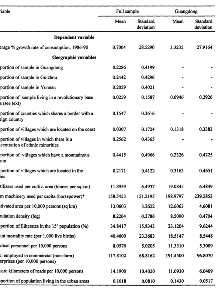
For the full sample over 1985-90, consumption per person grew at an average rate of only 0.70% per annum; for Guangdong, however, the rate of growth was 3.32% (Table 1). Between 1985 and 1990, 54% of the sampled households saw their consumption per capita increase while the rest experienced decline. If we confine our attention to Guangdong only, then we find that 68%

saw rising consumptions over the period.

The data appear to be of good quality. Since 1984 the RHS has been a well-designed and executed survey of a random sample drawn from a sample frame spanning rural China (including

small-medium towns), and with unusual effort made to reduce non-sampling errors (Chen and Ravallion, 1996). Sampled households fill in a daily diary on expenditures and are visited on

average every two weeks by an interviewer to check the diaries, and collect other data. There is also an elaborate system of cross-checking at the local level. The consumption data from such an intensive survey process are almost certainly more reliable than those obtained by the common cross-sectional surveys in which the consumption data are based on recall at a single interview. For the six year period 1985-90 the survey was also longitudinal, returning to the same

households over time. While this was done for administrative convenience (since local SSB offices were set up in each sampled county), the panel can still be formed.1_I

The consumption measure includes imputed values for consumption from own production valued at local market prices, and it an imputed value of the consumption streams from the inventory of consumer durables (Chen and Ravallion, 1996). Poverty lines designed to represent the cost at each year and in each province of a fixed standard of living were used as deflators. These were based on a normative food bundle set by SSB, which assures that average nutritional requirements are met with a diet which is consistent with Chinese tastes; this is valued at province-specific prices. The food component of the poverty line is augmented with an

allowance for non-food goods, consistent with the non-food spending of those households whose food spending is no more than adequate to afford the food component of the poverty line.'2

The household level data were collated with geographic data pertaining to three levels: the village, the county, and the province. At the village level, we have data on topography

" Constructing the panel from the annual RHS survey data proved to be more difficult than

expected since the identifiers could not be relied upon. Fortunately, virtually ideal matching variables were available in the financial records, which gave both beginning and end of year balances. The relatively few ties by these criteria could easily be broken using demographic data.

(whether the village is on plains, or in hills or mountains, and whether or not it is in a coastal

area), urbanization (whether it is a rural or suburban area), ethnicity (whether it is a minority

group village), whether or not it is considered a border area (three of the four provinces are at

China's external border), and whether or not the village is in a revolutionary base area (those

areas where the Communist Party had firmly established its bases prior to 1949). At the county level we have a much larger data base drawn from China's County Administrative Records, from

China's Rural county statistical year books for 1985-90, and from the 1982 Census.'3 These

cover agriculture (irrigated area, fertilizer usage, agricultural machinery in use), population density, average education levels, rural non-farm enterprises, road density, health indicators, and

schooling indicators. At the province level, we simply include dummy variables for the province. All nominal values are normalized by 1985 prices.

The survey data also allow us to measure a number of household characteristics. A

composite measure of household wealth can be constructed, comprising valuations of all fixed

productive assets, cash, deposits, housing, grain stock, and consumer durables. We also have data on agricultural inputs used, including landholding, and on the size and demographic compositions of the households, and levels of schooling.

13 While the county administrative records and the county yearbooks cover rural areas

separately, the census county data does not distinguish between the rural and urban areas. However, given that the objective of including the county characteristics is to proxy for the initial level of progress in a particular county relative to another, the aggregate county indicators should be reliable indicators for the differences in socio-economic conditions across the counties.

4 Results

We begin with a simple specification in which the only explanatory variables are initial value of wealth per capita, both at household and county levels. This model is too simple to be

believed, but it will help as an expository device for understanding a richer model later.

4.1 A simple expository model

Suppose that the only two variables that matter to the consumption growth rate are initial household wealth per capita. (HW) and mean wealth per capita in the county of residence (CW).

The growth model becomes:

Acil = a(1 -r, + r,Ac;,l + 9c(1 -r,)In CWt + 4(1 -r?lnHW, +residualit (9)

In interpreting this equation, it is useful to re-write it in the form:

Aci, =rAc tl + (1 -r,g(HW,, CW,) + residualt (10)

where

g(HWj, CW) =- a + 4ClnCW + ehlnHW

is interpretable as the balanced growth path implicit in (9).

The GMM estimate of this model gives r, values of 0.293, 0.258, 0.130, and 0.253 for

1987 to 1990 respectively. Using standard errors which are robust to any cross-sectional heteroscedasticity that might be present in the data, the corresponding t-ratios are 7.76, 7.95, 4.31, and 5.59. The estimated equation for the balanced growth rate is (t-ratios in parentheses,

also based on robust standard errors):

g(HW,CWM = -0.143- 0.0166lnHW + 0.03781nCW (11)

(5.61) (5.91) (8.13)

which is interpretable as the estimate of equation (3) implied by this specification, where HW is interpreted as a measure of K and CW as a measure of G.

Thus we find that consumption growth rates at the farm-household level are a decreasing function of own wealth, and an increasing function of average wealth in the county of residence,

controlling for latent heterogeneity. We can interpret equation (11) in terms of the model in section 2.1. The time preference rate and elasticity of substitution are not identified.

Nonetheless, given that the substitution parameter is positive, we can infer from equation (11) that the marginal product of own capital is decreasing with respect to own capital, but increasing

with respect to geographic capital. However, there are other possible interpretations; for example, credit might well be attracted to richer areas, or discount rates might be lower.

Notice that the sum of the coefficients on InCW and lnHW in (11) is positive. Thus, on averaging (11) over all households in a given county, we will find aggregate divergence; counties with higher initial wealth will tend to see higher subsequent average growth rates. However, this is due entirely to geographic externalities, rather than increasing returns to own wealth at the farm-household level.

4.2 A richer model

While the above specification is useful for expository purposes, we now want to extend the model by adding a richer set of both geographic and household level variables. Table I gives

the descriptive statistics of the explanatory variables to be used in an extended specification. Table 2 reports our GMM estimates of the extended model for both the sample as a whole and for Guangdong on its own. Again the conventional fixed effects model is firmly rejected in favor of the specification with time-varying coefficients.'4 _{This also means that we can estimate}

the impacts of the time-invariant geographic (and non-geographic) variables.

Our model also includes time-varying household variables, and one time-varying geographic (county-level) variable (Table 1). The question arises as to whether to treat these variables as exogenous or endogenous. We estimated a model where both the county and the household variables were assumed to be exogenous (base model). Next we estimated two alternative models: one where we assumed the county variables to be exogenous, but the time-varying household variables to be endogenous, and another where we assumed the time-time-varying county variable to be endogenous and the household variables to be exogenous. In both cases, we used lagged values as instruments. We then constructed likelihood ratio tests (Hall, 1993; Ogaki, 1993) to test the base model against these two models. The base model was summarily rejected in favor of the model where the time-varying household variables were endogenous, though the base model was accepted when tested against the model where the county variable was endogenous (and the household variables exogenous). Given these test results, Table 2 reports estimates where the time-varying household variables are treated as endogenous and the county variable as exogenous. All the time-invariant variables-county and household-are treated as exogenous. The likelihood ratio test gave similar results when we estimated the model

'4 Wald tests of the null hypothesis that each value of r, is unity gave Chi-square values of

for the households in Guangdong only.

Many of the geographic variables are significant, though not always the same variables for Guangdong as for the sample as a whole. Looking first at the results for the sample as a whole, we find that living in a revolutionary base area entails a higher growth rate than one would have otherwise expected. This suggests favorable treatment to these (historically

significant) areas by the center. While living in a coastal area has no significant effect controlling for other factors, living in a village in a mountainous area has a sizable and significant negative effect (a 0.9 percentage point lower annual growth rate), and living on the plains entails a

significantly higher growth rate ("hills" is the left out category). These results are consistent with better natural conditions for agriculture in the plains than mountains. Both of the

geographic variables which relate to the extent of modernization in agriculture (farm machinery usage per capita and fertilizer usage per acre) have highly significant positive impacts on

individual consumption growth rates. However, land under cultivation per capita does not. T'here is no significant effect of population density. Nor is there any sign that household consumption growth rates tend to be significantly higher in areas with higher proportions of

literate adults."5 The two health-related variables (infant mortality rate and medical personnel per capita) indicate that consumption growth rates at the farm-household level are significantly higher in generally healthier areas. A higher incidence of employment in non-farm commercial enterprises in a geographic area entails a higher growth rate at the household level for those living there. There is a highly significant positive effect of higher road density in an area on

consumption growth. The proportion of population living in urban areas has no effect. The quantitative magnitudes of these effects are not negligible. For example, a one standard deviation increase in farm machinery usage in an area adds 0.6 percentage points to the annual consumption growth rate holding all else constant; a one standard deviation increase in fertilizer usage adds 1.5 points; a one standard deviation increase in the density of medical personnel adds 0.5 (with presumably an additional impact via lower infant mortality), while a one standard deviation increase in rural road density adds 0.7 points.

The results are broadly similar for Guangdong, although some differences are notable. One expects some variables to become less significant due to the lack of variance within this one province. Unlike the sample as a whole, living in a revolutionary base area in Guangdong has no effect on the rate of consumption growth. Nor does living on the plains. Unlike the full sample, cultivated land per person is significant in Guangdong."6 Fertilizer usage is not. Population density emerges as a significant factor (possibly through an effect on local demand for non-farm goods and services, although it may also be picking up a tendency for other infrastructure variables to be better endowed in denser areas.) Infant mortality drops out in Guangdong, probably due to the lack of variance. However, access to medical personnel becomes even more significant. Road density also drops out if we confine attention to Guangdong.

Consistent with the simpler model we started with, there is a clear tendency amongst these geographic variables for their effects to be either neutral or "divergent", in that households have higher consumption growth rates in better endowed areas. This suggests that these

16 While the relatively low inequality in landholding may make it hard to identify this effect in

geographic characteristics tend to increase the marginal product of own capital.

This is in marked contrast to the household-level variables. In addition to allowing for latent farrn-household level effects on consumption growth, we included a number of household level characteristics related to land and both physical and human capital endowments. These effects tend to be convergent. Again focusing initially on the full-sample results, we find that farmn-households with higher expenditure on agricultural inputs per unit land area (an indicator of the capital intensity of agriculture) tended to have lower subsequent growth rates. Fixed

productive assets per capita do not, however, emerge as significant; it may well be that the density of agricultural inputs is the better indicator of own-farrn capital. Higher land per capita also results in a lower consumption growth rate.

Amongst the other household characteristics, there are a number of significant

demographic variables; larger and younger households tend to have higher consumption growth rates. This may reflect the thinness of agricultural labor markets in rural China, so that

demographics of the household influence the availability of labor for farrn work. There is a life-cycle effect, with growth rates increasing with age of the household head up to 44 years, and decreasing after that. Higher literacy amongst adults does not have a significant effect, although the proportion of children with secondary education has a significantly positive effect, and this may be picking up effects of human capital.

Again there are some differences between results for the full sample and those for GJuangdong. Fewer household demographic variables are significant in Guangdong, which suggests better-developed labor markets in rural areas of that province, which is plausible. There is a negative effect of higher incidence of primary school education in Guangdong, although the

left out category for this variable is all households with more than primary school education. So, the result should be interpreted as saying that all households with primary school education saw a drop in their consumption growth rates, compared to households with more than primary school education. Besides this variable, the only other household variable which has a significant impact on the consumption growth rate is the proportion of kids in the age-group 6-11 years.

4.3 Do spatialpoverty traps occur within the bounds of the data?

The above results are consistent with spatial poverty traps. But do such traps actually occur within the bounds of these data? In terms of the theoretical model in section 2.1, while one might find that higher endowments of geographic capital raise the marginal product of own

capital at the farm-household level, it may still be the case that no area has so little geographic capital as to entail falling consumption i.e., the marginal product of own capital in "poor areas" may still exceed the discount rate.

To address this issue, consider first our simple expository model in section 4.1. The poverty trap level of county wealth can be defined as CW* such that g(HW, CW*) = 0 for given HW. The sample mean of lnHW is 6.502 (with a standard deviation of 0.607). Then it is readily verified from equation (11) that lnCW' = 6.64, which is roughly mean log wealth. So if we consider two households with mean personal wealth, one living in a county with slightly above average wealth, the other in one with below average wealth, then our results imply that the former household will see its consumption rising, while it will be falling for the latter. Spatial poverty traps are clearly well within the bounds of these data.

Following the samne approach, we can ask the same question for the richer model. We calculate the critical value of each geographic variable at which consumption growth is zero

while holding all other (geographic and non-geographic) variables constant at their sample mean values. The critical values implied by our results are given in Table 3. We find, for example,

that positive growth in consumption requires that the density of roads exceeds 8.9 square

kilometers per 10,000 people (with all other variables evaluated at mean points). In all cases, the

critical value at which the spatial poverty trap arises is within one standard deviation of the

sample mean for that characteristic.

5 Conclusions

Mapping poverty and its correlates could well be far more than a descriptive tool-it may also hold the key to understanding why poverty persists in some areas, even with robust

aggregate growth. That conjecture is the essence of the theoretical idea of a spatial poverty trap.

But are such traps of any empirical significance?

Aggregate growth empirics cannot answer that question, since aggregation confounds the external effects that create spatial poverty traps with purely internal effects. And, without controlling for latent heterogeneity in the micro growth process, it is hard to accept any test for spatial poverty traps based on micro panel data. In a regression for consunption growth at the household level, significant coefficients on geographic variables may simply pick up the effects of omitted spatially-autocorrelated household characteristics. Yet the standard treatments for fixed effects in micro panel-data models make it impossible to identify the impacts of the many time-invariant geographic factors that one might readily postulate as leading to spatial poverty

traps. Given the potential policy significance of poverty traps, it is worth searching for a

convincing method to test for them.

We have offered a test. This involves regressing consumption growth at the household

level on geographic variables, allowing for nonstationary individual effects in the growth rates. By relaxing the restriction that the individual effects have the same impacts at all dates, the

resulting dynamic panel-data model of consumption growth allows us to identify external effects

of fixed or slowly changing geographic variables. The model can be estimated by the

Generalized Method of Moments.

On implementing the test on farm-household panel data for rural areas of southern China,

we find strong evidence that a number of indicators of geographic capital have divergent impacts on consumption growth at the micro level, controlling for (observed and unobserved) household characteristics. The main interpretation we offer for this finding is that living in a poor area

lowers the productivity of a farm-household's own investments, although we note other possible explanations such as geographic differences in access to credit or in preferences.

The geographic effects we find are strong enough to yield spatial poverty traps. Our

results suggest that there are areas in this part of rural China which are so poor that the

consumptions of some households living in them will be falling even while otherwise identical

households living in better off areas enjoy rising consumptions. By interpretation, equilibriurn growth paths in poor areas entail that the marginal products of own capital for at least some farm households living there are lower than their discount rates.

What geographic characteristics create such spatial poverty traps? We find that there are

in living standards. We also find, however, that the aspects of geographic capital relevant to consumption growth embrace both private and publicly provided goods and services. Private

investments in agriculture, for example, entail external benefits within an area, as do "mixed"

goods (involving both private and public provisioning), such as health care. The prospects for

growth in poor areas will then depend on the ability of governments and community

organizations to overcome the tendency for under-investment that such geographic externalities

Appendix: GMM estimation of the micro growth model

The estimation procedure entails stacking the equations in (8) to form a cross-section system, with one equation for each year. For T=6, the system of equations to be estimated is as

follows:

q3 (A Cj3, X, z, b3) ui3

q4(Ac.4, Xz4, Zib4) = Ui4 (Al)

q5s( c5, Xijs zi, b5) U=5 q6(AC 6 Xi6' z,b1 6) uj6

In these equations, u, (t=3,4,5,6) is the error term u ₁₁-r, u;,, -, x,, is the vector of time-varying

explanatory variables, z, the vector of time invariant variables, and bt = [a,

J,

restrictions on the parameters. It is convenient to write the model in the compact form:

q(Ac,1x1,z ,,b) = i (A2)

where = [ii3uiI 4ui uI ,

I-The GMM procedure estimates the parameters b, by minimizing the criterion function:

QNT(b) = gN(b)'AN1 gN(b) (A3)

where the (r x r% h aNN- is positive definite, and where the (r x 1) vector of sample

N

gN(b) = [w2 Wl1(Ac, x;, z;, b)] (A4)

where w, is a (1 xp) vector of p instruments. Heteroscedasticity is likely to exist across the

cross-sections. We use White's approach to correct for this. The optimal weighting matrix is thus the inverse of the asymptotic covariance matrix:

N

AN = W (A5)

5=1

where z2u is the vector of the estimated residuals. These GMM estimates yield parameter

estimates that are robust to heteroscedasticity.

The first-order conditions of minimizing equation QN,(b) imply that S is the solution to:

GN(S)AN gN(b) = ° (A6)

where G N(£) is the (r x q) matrix with its (i, j)th element GN(b) j.a=g ni .(b) /ab and gn, (b) is the

i 'th element of gN(b). GN(b) is assumed to be of full rank. However, given the nonlinearity in

the criterion function, equation (A6) does not provide us with an explicit solution. We must use

a numerical optimization routine to solve for S. All the computations can be done using (say)

References

Azariadis, Costas, 1996, "The Economics of Poverty Traps. Part One: Complete Markets",

Journal of Economic Growth, 1: 449-486.

Barro, Robert J., and Xavier Sala-i-Martin, 1992, "Convergence", Journal of Political Economy, 100: 223-252.

Borjas, George, 1995, "Ethnicity, Neighborhoods, and Human Capital Externalities", American

Economic Review 85: 365-380.

Chen, Shaohua and Martin Ravallion, 1996, "Data in Transition: Assessing Rural Living Standards in Southern China", China Economic Review, 7: 23-56.

Hall, A. (1993), "Some Aspects of Generalized Method of Moments Estimation", in G. S. Maddala, C. R. Rao, and H. D. Vinod (eds) Handbook of Statistics, Volume 11, North-Holland.

Holtz-Eakin, D., W. Newey and H. Rosen, 1988, "Estimating Vector Autoregressions with Panel Data", Econometrica, 56: 1371-1395.

Jalan, Jyotsna and Martin Ravallion, 1997a, "Transient and Chronic Poverty in Rural China: A Semiparametric Estimation", mimeo, Development Research Group, World Bank.

. and ,

1997b,

Development Program?", Journal of Public Economics, in press.

Leading Group, 1988, Outlines of Economic Development in China's Poor Areas, Office of the Leading Group of Economic Development in Poor Areas Under the State

Council, Agricultural Publishing House, Beijing.

Economics, 12, 3-42.

Ogaki, M. (1993), "Generalized Method of Moments: Econometric Applications", in G. S.

Maddala, C. R. Rao, and H. D. Vinod (eds) Handbook of Statistics, Volume 11,

North-Holland.

Ravallion, Martin, 1997, "Poor Areas", in Giles, David and Aman Ullah (eds) Handbook of

Applied Economic Statistics, New York: Marcel Dekkar (in press).

Ravallion, Martin and Jyotsna Jalan, 1996, "Growth Divergence due to Spatial Externalities",

Economics Letters, 53(2): 227-232.

Romer, Paul M., 1986, "Increasing Returns and Long-Run Growth", Journal of Political

Economy, 94:1002-1037.

World Bank, 1992, China: Strategies for Reducing Poverty in the 1990s, World Bank,

Table 1: Descriptive statistics

Variable Full sample Guangdong

Mean Standard Mean Standard deviation deviation Dependent variable

Average % growth rate of consumption, 1986-90 0.7004 28.5290 3.3235 27.9164 Geographic variables

Proportion of sample in Guangdong 0.2286 0.4199 -

-Proportion of sample in Guizhou 0.2442 0.4296

-Proportion of sample in Yunnan 0.2029 0.4021 -

-Proportion of sample living in a revolutionary base 0.0259 0.1587 0.0946 0.2926 area (see text)

Proportion of counties which shares a border with a 0.1547 0.3616

-foreign country

Proportion of villages which are located on the coast 0.0307 0.1724 0.1318 0.3383 Proportion of villages in which there is a 0.2562 0.4365

-concentration of ethnic minorities

Proportion of villages which have a mountainous 0.4415 0.4966 0.2326 0.4225 terrain

Proportion of villages which are located in the 0.2171 0.4122 0.3163 0.4651 plains

Fertilizers used per cultiv. area (tonnes per sq.km) 11.8959 6.4937 19.0845 6.4849 Farm machinery used per capita (horsepower)* 158.5453 151.2195 198.9797 239.2853 Cultivated area per 10,000 persons (sq km) 13.0603 3.2622 12.6063 4.6081

Population density (log) 8.2264 0.3786 8.5090 0.4704

Proportion of illiterates in the 15+ population (%) 34.8417 15.8343 23.1204 9.6244 Infant mortality rate (per 1,000 live births) 40.4600 23.3683 18.5147 8.5448 Medical personnel per 10,000 persons 8.0576 5.0205 11.3310 5.3009 Pop. employed in commercial (non-farm) 117.8102 68.8162 191.4500 96.8070

enterprises (per 10,000 persons)

Square kilometers of roads per 10,000 persons 14.1900 10.4020 11.0930 6.0409 Proportion of population living in the urban areas 0.1018 0.0810 0.1430 0.0517

Variable Full sample Guangdong Mean Standard Mean Standard

deviation deviation

Household level variables

Expenditure on agricultural inputs (fertilizers & 30.4597 80.5274 60.8067 154.4674 pesticides) per cultivated area (yuan per mu)*

Fixed productive assets per capita (yuan per capita)* 132.1354 217.5793 125.0693 256.0311 Cultivated land per capita (mu per capita)* 1.2294 1.1011 0.9882 0.6476

Household size (log)* 1.6894 0.3461 1.7027 0.3350

Age of the household head 42.1315 11.4225 43.6147 11.0557 '*

Age2of the household head 1,905.5300 1,024.7320 2,024.4600 1,018.8200 Proportion of adults-in the household who are 0.3230 0.2898 0.2163 0.2353 illiterate

Proportion of adults in the household with primary 0.3819 0.3063 0.4210 0.2970 school education

Proportion of kids in the household between ages 0.1173 0.1408 0.1101 0.1426 6-11 years

Proportion of kids in the household between ages 0.0836 0.1066 0.0763 0.1051 12-14 years

Proportion of kids in the household between ages 0.0698 0.1004 0.0740 0.1018 15-17 years

Proportion of kids with primary school education 0.2672 0.3642 0.2500 0.3581 Proportion of kids with secondary school education 0.0507 0.1757 0.0747 0.2227 Proportion of a household members working in the 0.0436 0.2042 0.0558 0.2296 state sector

Proportion of 60+ household members 0.0637 0.1218 0.0601 0.1055 Notes: * indicates that the variable is time-varying in the GMM model. 1 mu = 0.000667 km2

Table 2: Estimates of the consumption growth model

Full sample Guangdong

Coeff. estimate t-ratio Coeff. estimate t-ratio

Constant -0.2820 -3.1625* -1.3575 -5.8606*

Time-varying fixed effects

r8, 0.0399 1.4653 0.1239 2.8878* 0.2269 7.5543* 0.1231 2.4650* r.9 0.0981 3.6426* 0.2969 4.5375* r90 0.4871 11.8983* 0.2979 4.2699* Geographic variables Guangdong (dummy) 0.0040 0.7323 - -Guizhou (dummy) 0.0226 4.2838* Yunnan (dummy) -0.0035 -0.5749 -

-Revolutionary base area (dummy) 0.0256 2.7725* -0.0118 -1.1250

Border area (dummy) -0.0015 -0.3318 -

-Coastal area (dummy) -0.0132 -1.5117 0.0024 0.2771

Minority area (dummy) -0.0034 -0.9705 -

-Mountainous area (dummy) -0.0090 -2.5859* -0.0204 -2.6576*

Plains (dummy) 0.0105 2.7136* -0.0079 -1.1120

Farm machinery usage per capita (xlOOO) 0.0420 3.4328* 0.0597 3.9327* Cultivated area per 10,000 persons 0.0013 1.5013 0.0109 4.8882* Fertilizer used per cultivated area 0.0023 4.5678* 0.0002 0.2615

Population density (log) 0.0160 1.6949 0.1308 5.8433*

Proportion of illiterates in 15' population (xlOO) 0.0159 0.9000 0.0467 1.2352 Infant mortality rate (xl OO) -0.0313 -2.5295* -0.0422 -0.8071 Medical personnel per capita 0.0011 3.6882* 0.0054 8.2851* Prop. of pop. empl. nonfarm commerce (xlOO) 0.0067 2.1156* 0.0130 2.4340* Square kilometers of roads per capita (xlOO) 0.0741 4.3033* 0.0849 1.3341 Prop. of population living in the urban areas -0.0228 -1.0254 -0.3080 -3.3753*

Full sample Guangdong

Coeff. estimate t-ratio Coeff. estimate t-ratio Household level variables

Expenditure on agricultural inputs per cultivated -0.1193 -5.6113* -0.0171 -1.6459 area (xlOO)

Fixed productive assets per capita (x 1000) 0.0042 0.3048 0.0324 1.4772 Cultivated land per capita -0.0151 -2.6279* -0.0149 -1.4027

Household size (log) 0.0473 6.9675* 0.0334 2.6298*

Age of the household head (x 100) 0.2324 2.8321* 0.0357 0.2121 Age2 of the household head (x 100) -0.0026 -2.9200* -0.0001 -0.0629 Proportion of adults in the household who are 0.0079 1.2696 -0.0069 -0.5126

illiterate

Prop. of adults in the h'hold with primary school -0.0040 -0.7948 -0.0207 -2.2251 *

education

Prop. of kids in the household between ages 6- 0.0330 3.4658* 0.0450 2.4429* 11 years

Prop. of kids in the h'hold between ages 12-14 0.0421 3.1405* 0.0458 1.8187

years

Prop. of kids in the h!hold between ages 15-17 0.0096 0.6185 0.0136 0.4990 years

Proportion of kids with primary school -0.4348 -1.0644 -0.0041 -0.0047

education (x 100)

Proportion of kids with secondary school 0.0209 2.4275* 0.0090 0.6972 education

Whether a household member works in the state -0.0132 -1.8790 -0.0150 -1.3721 sector (dummy)

Proportion of 60+ household members 0.0189 1.5487 -0.0205 -0. 6738 Notes: *: indicates significant at 5% level or better

Table 3: Critical values for a spatial poverty trap

Full sample Guangdong

Critical values to Sample mean Critical values to Sample mean Geographic variables avoid spatial (standard avoid spatial (standard

poverty traps deviation in poverty traps deviation in

parentheses) parentheses)

Cultivated area per 10,000 persons - - 12.3861 12.606

(sq km.) (4.608)

Fertilizers used per cultivated area 10.1650 11.896

-(tonnes per sq km) (6.494)

Farm machinery used per capita 65.6550 158.545 158.6500 198.980

(horsepower) (151.220) (239.285)

Population density (log) - - 8.4906 8.509

(0.470) Infant mortality rate (per 1,000 live 52.9245* 40.460

-births) (23.368)

Medical personnel per 10,000 4.4783 8.058 10.8852 11.331

persons (5.020) (5.301)

Population employed in 59.3186 117.810 172.9294 191.450

commercial (non-farm) enterprises (68.816) (96.807)

(per 10,000 persons)

Square kilometers of roads per 8.9250 14.190

-10,000 persons (10.402)

Proportion of population living in - 0.1508* 0.143

urban areas (0.052)

Notes: A spatial poverty trap will exist if the observed value for any county is less than the critical values given above; for those marked * the observed value cannot exceed the critical value if a poverty trap is to be avoided. Critical values are only reported if the relevant coefficient from Table 2 is significantly different from zero. All the critical values reported above are significantly different from zero (based on a Wald-type test) at the 5% level or better.

Policy Research Working Paper Series

Contact

Title Author Date for paper

WPS1842 Motorization and the Provision of Gregory K. Ingram November 1997 J. Ponchamni

Roads in Countries and Cities Zhi Liu 31052

WPS1843 Externalities and Bailouts: Hard and David E. Wildasin November 1997 C. Bernardo

Soft Budget Constraints in 37699

Intergovernmental Fiscal Relations

WPS1 844 Child Labor and Schooling in Ghana Sudharshan Canagarajah November 1997 B. Casely-Hayford

Harold Coulombe 34672

WPS1845 Employment, Labor Markets, and Sudharshan Canagarajah November 1997 B. Casely-Hayford

Poverty in Ghana: A Study of Dipak Mazumdar 34672

Changes during Economic Decline and Recovery

WPSI 846 Africa's Role in Multilateral Trade Zhen Kun Wang November 1997 J. Ngaine

Negotiations L. Alan Winters 37947

WPS1 847 Outsiders and Regional Trade Anju Gupta November 1997 J. Ngaine Agreements among Small Countries: Maurice Schiff 37947 The Case of Regional Markets

WP81848 Regional Integration and Commodity Valeria De Bonis November 1997 J. Ngaine

Tax Harmonization 37947

WPS1 849 Regional Integration and Factor Valeria De Bonis November 1997 J. Ngaine

Income Taxation 37947

WPS1850 Determinants of Intra-Industry Trade Chonira Aturupane November 1997 J. Ngaine

between East and West Europe Simeon Djankov 37947

Bernard Hoekman

WPS1851 Transportation Infrastructure Eric W. Bond November 1997 J. Ngaine

Investments and Regional Trade 37947

Liberalization

WPS1852 Leading Indicators of Currency Graciela Kaminsky November 1997 S. Lizondo

Crises Saul Lizondo 85431

Carmen M. Reinhart

WPS1 853 Pension Reform and Private Pension Monika Queisser November 1997 P. Infante

Funds in Peru and Colombia 37642

WPS1854 Regulatory Tradeoffs in Designing Claude Crampes November 1997 A. Estache

Concession Contracts for Antonio Estache 81442

Infrastructure Networks

Policy Research Working Paper Series

Contact

Title Author Date for paper

WPS1856 Surviving Success: Policy Reform Susmita Dasgupta November 1997 S. Dasgupta

and the Future of Industrial Hua Wang 32679

Pollution in China David Wheeler

WPS1857 Leasing to Support Small Businesses Joselito Gallardo December 1997 R. Garner

and Microenterprises 37664

WPS1 858 Banking on the Poor? Branch Martin Ravallion December 1997 P. Sader

Placement and Nonfarm Rural Quentin Wodon 33902

Development in Bangladesh

WPS1859 Lessons from Sgo Paulo's Jorge Rebelo December 1997 A. Turner Metropolitan Busway Concessions Pedro Benvenuto 30933 Program

WPS1860 The Health Effects of Air Pollution Maureen L. Cropper December 1997 A. Maranon

in Delhi, India Nathalie B. Simon 39074

Anna Alberini P. K. Sharma

WPS1861 Infrastructure Project Finance and Mansoor Dailami December 1997 M. Dailami Capital Flows: A New Perspective Danny Leipziger 32130