Estimation of Distribution Algorithms to Test
Concurrent Software
Jan Staunton and John A. Clark
Department of Computer Science, University of York, UK {jps,jac}@cs.york.ac.uk
Abstract. Previous work has shown the efficacy of using Estimation of Distribution Algorithms (EDAs) to detect faults in concurrent soft-ware/systems. A promising feature of EDAs is the ability to analyse the information or model learned from any particular execution. The analysis performed can yield insights into the target problem allowing practitioners to adjust parameters of the algorithm or indeed the algo-rithm itself. This can lead to a saving in the effort required to perform future executions, which is particularly important when targeting expen-sive fitness functions such as searching concurrent software state spaces. In this work, we describe practical scenarios related to detecting con-current faults in which reusing information discovered in EDA runs can save effort in future runs, and prove the potential of such reuse using an example scenario. The example scenario consists of examining problem families, and we provide empirical evidence showing real effort saving properties for three such families.
1
Introduction
Estimation of Distribution Algorithms (EDAs) have been established as a strong competitor to Evolutionary Algorithms (EAs) and other bio-inspired techniques for solving complex combinatorial problems [8]. EDAs are similar to Genetic Algorithms (GAs), but replace the combination and mutation phases with a probabilistic model building and sampling phase. It has been shown that EDAs can outperform GAs on a range of problems. In addition to strong performance, another advantage of EDAs is the potential for the analysis of the probabilistic models constructed at each generation. Model analysis can yield insights into a target problem allowing for tuning of EDA parameters, or indeed the algorithm itself, potentially saving computation effort in future instances.
Recently, we have shown the potential for EDAs, combined with aspects of model checking, to detect faults in concurrent software by sampling the state-space of the program intelligently [11,12]. Using a customised version of N-gram GP [9], we have achieved greater performance than a number of traditional algorithms, GAs and Ant Colony Optimisation (ACO) on a wide range of prob-lems, including programs expressed in industrial languages such as Java. For
M.B. Cohen and M. ´O Cinn´eide (Eds.): SSBSE 2011, LNCS 6956, pp. 97–111, 2011. c
large problems, exploring the state-space can become expensive, leading to a longer runtime and the potential exhaustion of resources. In order to combat this effect, we propose using information, specifically information from the mod-els constructed, from earlier executions of the EDA in future executions in an attempt to save computational effort. We term this approach “model reuse”.
In this work, we outline practical scenarios related to detecting faults in con-current software in which model reuse could potentially save computation effort. These scenarios could potentially be extended to scenarios involving sequen-tial software, and even hardware systems. We then provide empirical evidence showing the potential of model reuse with regards to detecting faults in problem families. A problem family is a program or system that can be scaled up or down with respect to some parameter, typically the number of processes within the system. Our system is implemented using the ECJ evolutionary framework [7] and the HSF-SPIN model checker [5]. To our knowledge, this is the first instance of model analysis being used to save computational effort, and therefore lower cost, in the Search-Based Software Engineering (SBSE) domain.
This paper is structured as follows: Section 2 gives a brief overview of how EDAs and the EDA-based model checking technique work. Section 3 describes the concept of model reuse, along with a number of practical scenarios in which model reuse could reduce computational effort. Section 4 describes empirical work showing the potential for model reuse in practical scenarios. We conclude the paper with a summary and outline future work in Section 5.
2
EDA-Based Model Checking
2.1 EDAs
Estimation of Distribution Algorithms (EDAs) are population-based probabilis-tic search techniques that search solution spaces by learning and sampling proba-bilistic models [8]. EDAs iterate over successive populations or bags of candidate solutions to a problem. Each population is sometimes referred to as a genera-tion. To construct a successor population, EDAs build a probabilistic model of promising solutions from the current population and then sample that model to generate new individuals. The newly generated individuals replace individuals in the current population to create the new population according to some replace-ment policy. An example replacereplace-ment policy is to replace half of the old popula-tion with new individuals. The initial populapopula-tion can be generated randomly, or seeded with previously best known solutions. The algorithm terminates when a termination criterion is met, typically when a certain number of generations are reached or a good enough solution has been found.
The pseudocode of a basic EDA algorithm is shown in Algorithm 1. Readers who are familiar with Genetic Algorithm (GA) literature can view EDAs as similar to a GA with the crossover and mutation operators replaced with the model building and sampling steps. EDAs can be seen as strategically sampling the solution space in an attempt to find a “good” solution whilst learning a model of “good” solutions along the way. EDAs are sometimes referred to as
Algorithm 1.Pseudocode for basic EDA
P = InitialPopulation(); evaluate(P);
whilenot(termination criterion)do
S = SelectPromisingSolutions(P); M = UpdateModelUsingSolutions(S); N = SampleFromModel(M); P = ReplaceIndividuals(N); evaluate(P); end while
Probabilistic Model-Building Genetic Algorithms (PMBGAs), a full overview of which can be found in [8].
2.2 Searching State-Spaces with EDAs
To search for concurrent faults using EDAs, we use aspects of model checking. Model Checking is a technique for analysing reactive concurrent systems [4]. A model checking tool can automatically verify that a given specification is satisfied by a model of a system. A model checking tool achieves this by taking a descrip-tion of a system and a specificadescrip-tion, and then exhaustively checks all possible be-haviours of that system to determine if the specification is violated. The descrip-tion of the system can be in a number of formats, including being expressed in industrial languages such as Java. Specifications are given as a set of properties and are typically expressed in a formal language such as Linear Temporal Logic (LTL). Example specifications include “The system must not deadlock” and “The server must respond once a request has been made by a client”.
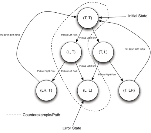
A possible behaviour of a system is typically referred to as a path. A pathp is a sequence of states which begins in an initial state of the system/program, and ends in either a terminal state (a state from which no transition can occur) or a state previously encountered onp. A path can also be seen as a sequence of actions causing transitions between states. A transition system/state space is shown in Figure 1, showing all of the main features pertinent to this work. The goal of a model checking tool is to find a path that violates a given specification, known as a “counterexample”. This goal is typically achieved using a Depth-first Search. If no such path exists in the system after an exhaustive check, then the system is said to satisfy the specification. For large systems, however, it is often impossible to check all possible paths due to a lack of time and memory. This is known as the state-space explosion problem [4]. In these situations, it may suffice to detect a counterexample rather than check the system exhaustively. For this purpose, a number of heuristic mechanisms exist. Best-first Search for instance expands states during the search in an order determined by a heuristic [5]. Heuristics exist for searching for a variety of faults [6,5], including deadlock and violations of LTL formulae. Counterexamples with fewer states are often pre-ferred for debugging purposes, as superfluous transitions are eliminated. To this end techniques including A* search can be used that penalise longer paths [10].
(T, T)
(L, T) (T, L)
(LR, T) (L, L) (T, LR)
Pickup Left Fork Pickup Left Fork
Pickup Right Fork
Pickup Right Fork Pickup Left Fork
Pickup Left Fork
Initial State
Error State Counterexample/Path
Put down both forks
Put down both forks
Fig. 1.Figure of a Dining Philosopher transition system/state space visualised as a digraph. States are shown as circles, with edges between them labelled with actions on the left. The path highlighted is a counterexample that leads to a deadlock state.
Metaheuristic mechanisms have been shown to be promising when used to de-tect faults in concurrent software/systems. Genetic Algorithms have been shown to be effective at detecting deadlock in Java programs [3]. Ant Colony Optimisa-tion has also been shown to be effective at detecting a variety of different errors types, including deadlock and LTL formulae violations [1,2], in Promela models. Recently, we have shown how an EDA-based model checking algorithm based upon N-gram GP can be used to discover short errors in concurrent systems [11,12]. Using this work, we show how the algorithm described in [11,12] can be modified to allow for information in previous runs to save computational effort in later runs. Our system is implemented using ECJ [7] and SPIN [5]. HSF-SPIN is a model checking framework that analyses Promela specifications, and implements a variety of heuristics for checking a range of properties.
2.3 Brief Overview of EDA-Based Model Checking
Before a description of the technique is given, it helps to summarise the overall theme. The goal of the EDA is to detect a path in the transition system which leads to a fault. To this end, the EDA samples a set of paths from the transition system (referred to as a population) and selects a subset of “fit” paths determined by a fitness function. Using the individuals in the fit subset, a probabilistic model is constructed. The model is then sampled in order to construct new paths which replace current members of the population. In order to generate new paths, the model is built so that it can answer the following the question. Given thenmost recent actions that have occurred on the path currently under construction, by what distribution should the next action be selected? The model can be thought of as a strategy for navigating a transition system.
Solution Space. In order to encode paths in the transition system, we use a simple string representation. Paths in a transition system can be seen as a se-quence of actions causing transitions between states. The alphabet of the strings used in this work is the set of all actions possible in the transition system. In this work, the alphabet consists of information gathered by HSF-SPIN whilst constructing the transition system. Examples of the alphabet members used in this work can be found in Figure 2, which shows a typical path through a Dining Philosophers transition system. The alphabet members do not refer to specific philosophers, but instead refer to actions that can be performed by any one of the philosophers in the system. By modelling paths through a transition sys-tem without referring to specific processes, sequences of actions regardless of which processes executed them are modelled. This represents a minor abstrac-tion from modelling acabstrac-tions performed by specific processes, reducing the size of the alphabet and therefore reducing the solution space searched by the EDA.
1 . (NULL TRANSITION)
2 . ( m od e ls / d e a d l o c k . p h i l o s o p h e r s . n o l o o p . prm : 3 2 ) ( b r e ak ) 3 . ( m od e ls / d e a d l o c k . p h i l o s o p h e r s . n o l o o p . prm : 1 2 ) ( l e f t ? f o r k ) 4 . ( m od e ls / d e a d l o c k . p h i l o s o p h e r s . n o l o o p . prm : 1 2 ) ( l e f t ? f o r k )
Fig. 2.A typical trace/string/path from HSF-SPIN on the Dining Philosopher problem with 2 philosophers. This trace ends in a deadlocked state, because all the philosophers have picked up their left fork.
Modelling Paths. In order to model paths in the transition system, we use a customised version of N-gram GP [9]. An n-gram is a subsequence of length nfrom a longer sequence. N-gram GP learns the joint probabilities of fit string subsequences of lengthn. The rationale is that N-gram GP is modelling a strat-egy to use whilst exploring a transition system. The n-grams are seen as a recent history of actions on a particular path. The distribution associated with the n-gram in the probabilistic model describes the actions that are most likely to minimise a fitness function, hopefully leading to a counterexample. The model
is “queried” with n-grams during the sampling phase in order to probabilistically choose actions that are more likely to lead to a fault.
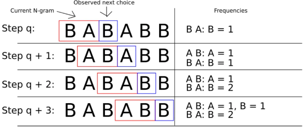
For each generation a set of “fit” paths is selected using truncation selection and the fitness function described later in this work. In order the learn the model or strategy from a set of fit paths, a simple sliding window frequency count algo-rithm is used. Once the paths are selected, a frequency count of actions occurring after each unique n-gram in the paths is performed. The frequency count is then normalised to obtain distributions for each n-gram observed. A simple illustra-tion of this process can be seen in Figure 3. In addiillustra-tion to learning n-gram distributions, in this work the distributions for (n-1)-grams and (n-2)-grams etc. down to 1-grams are also constructed and these additional distributions are used during the sampling phase.
!
!"
!"
!"#
Fig. 3.Illustration of the N-gram learning process (2-grams in this case). A frequency count is performed for each unique N-gram in the selected set of strings (only one string is shown). The boxes represent a basic sliding window algorithm, with frequency counts display on the right.
Sampling the Model. Once a set of individuals are selected and a model created, the model is then sampled to create the next generation. A number of paths are generated from the model to replace individuals in the current generation according to some policy. In this work, we generate the entire new generation using newly sampled individuals. To generate a path in the transition system, the algorithm starts with the initial state of the transition system and an empty path. Then, the algorithm must choose an action to execute from the available actions in the current state. To do this, the model is queried with the most recent n moves from the path, in this case an empty string, and a distribution is returned. From the initial state, a set of actions are possible, each of which leads to a potentially new state. Using the distribution obtained from the model for the current n-gram, an action is probabilistically chosen and executed. If more than one process is in a position to execute the chosen action, then a single process is selected at random from those that can execute the chosen
action at random to progress. This leads to a new state s. The action chosen is appended to the current path, and the process is repeated using the new state and the new path. This process repeats until either an error is found, a terminal state is reached or a state is reached that has been previously encountered on the current path.
N-gram GP was initially used to evolve programs, allowing any sequence of alphabet members to constitute a program. However, in this work we must gen-erate valid paths in the transition system. If we used the process described above without modification, it is entirely possible to generate invalid paths in the tran-sition system. There are a number of special cases when generating a path, and these are described and handled in [11]. Mutation is implemented by taking an arbitrary choice everymtransitions according to some parameter.
3
Model Reuse
A typical GA run will produce a sequence of bags of solutions to a target problem. In the case of detecting concurrent faults, this will amount to sets of paths within the transition system which may or may not lead to an error. Whilst it is possible to use some of these solutions to seed future runs, even a small change to the target problem could destroy the applicability of these solutions. Similarly, Ant Colony Optimisation constructs pheromone trails that may lose relevance once the target problem has been changed. The EDA-based model checking technique, on the other hand, produces a strategy for navigating a transition system in addition to structures that represent solutions. We believe that with some simple steps the models can be used to reduce computational effort on future instances of similar problems. Outlined below are a number of potential practical scenarios for model reuse that could greatly reduce computational effort.
3.1 Reuse during Debugging
The first proposed scenario for model reuse is during the testing/debugging phases of the development life cycle. It is plausible that during any execution of the EDA a constructed model can represent a strategy for finding not just a single error but multiple errors, as well as “problem areas” of the state space. If a single error has been found in an execution e on the ith revision of the system,ecould be halted in order to fix the bug. This would create the i+ 1th revision. Once the error has been corrected, execution can continue using the model constructed in the last generation of e, labelled m. It is also plausible that erroneous actions from theith revision of the system inmcan be mapped to the corrected actions in the revised system, allowing for the EDA to focus on these areas initially. This may potentially eliminate computation if errors still exist in the area of the state space where the initial error was found. Equally, if a practitioner is confident that the error has been corrected, the area of the state space can be added to a tabu list, allowing the EDA to focus effort elsewhere.
3.2 Reuse during Refinement
Another potential scenario for reusing models is during refinement. During im-plementation, versions of the system are refined to meet various ends, including performance improvements and bug fixing. Refinements may increase the size of the transition system enormously. In order to combat this, it is plausible that the EDA can be executed on the more abstract version of the system/software in order to determine potential problem areas that rank highly with the fit-ness function. The models constructed during these initial explorations can then potentially be used to explore future refinements of the system. If refining the system increases the state space size significantly, then significant computational effort could be spared. There is also the potential to map actions from the ab-stract system to actions in the refined system, potentially increasing the saving of computational effort.
3.3 Reuse When Tackling Problem Families
We have speculated in previous papers [11,12] that the EDA-based technique is learning effective strategies for navigating the state spaces of problem families, rather than just the problem instance itself. A problem family is simply a sys-tem which can be scaled up and down respective to some parameter, typically the number of processes/threads in the system/software. This opens up the pos-sibility of models learned whilst tackling small instances of a problem family can be used to save effort whilst finding errors in larger instances. Finding the same error in a number of instances of a problem family can provide additional debugging information, potentially shortening the debugging life cycle. Problem families arise frequently in practical situations [4], in both hardware and software systems.
In this work, we provide empirical evidence showing how computational effort can be saved when detecting errors in problem families. Extra information can be gained from detecting faults in varying instances of a problem family, and this can save time and ultimately lower costs when building and debugging practical systems.
4
Experimentation with Problem Families
4.1 Sample Models
In order to demonstrate the ability for model reuse, we aim to show that the EDA can learn structures in three problem families. The three test cases used in this work are listed in Table 1. The test cases are diverse in the system description as well as the property under test. The dining philosophers model is a classic problem in whichnphilosophers contend over forks in order to eat from a shared meal in the middle.nphilosophers are sat around a circular table withnforks, one between each adjacent pair of philosophers. Each philosopher requires two forks in order to eat. Each philosopher picks up the fork to the left of them,
then the fork to the right, eats some food, then releases the right and left fork in that order. With this behaviour, there is the possibility of deadlock as all philosophers can pick up the left fork denying access to the right fork for every philosopher. The EDA will be aiming to find deadlocked states within the dining philosopher model.
Table 1.Models and the respective properties violated
Model Processes LoC Property
Dining Philosopher No Loopnn+ 1 35 Deadlock
Leadern n+ 1 117 Assertion
GIOPn n+ 6 740 (p→♦q)
For the second test case, a leader election system is modelled by the Leader model. In this model,nprocesses must agree on a common leader process in a unidirectional ring configuration. The faulty protocol used to establish a leader allows members of the ring to disagree on a leader. An assertion represents this specification, and the EDA algorithm will be aiming to find violations of this assertion. The final test case implements the CORBA Global Inter-ORB protocol (GIOP) with nclients using a single server configuration. The system violates a property specified in LTL. This model is particularly large, and is reported as difficult to find errors in for largen(largenbeing n >= 10) [2,12].
In this set of examples, we have a deadlock, an assertion and an LTL violation in order to show the applicability of the technique to errors other than deadlock. Whilst the Dining Philosophers problem is a well studied toy problem, the GIOP model is derived from an industrial source, adding credibility to using this ap-proach in industrial scenarios. Finally, whilst the Dining Philosophers model is symmetrical in nature (all the processes have the same description), the GIOP model is asymmetric, adding further weight to the empirical argument that the technique could be effective in industrial scenarios.
4.2 Heuristics
The fitness function detailed in Algorithm 2 is used to rank solutions and makes use of heuristic information implemented in the HSF-SPIN framework [5]. The heuristics implemented in HSF-SPIN give information about a single state only. Algorithm 3 combines the information from the individual states in a path to give a heuristic measure for the entire path. This is done by simply summing the heuristic information of all the states along the path. The algorithm aims to minimise this cumulative total, whilst favouring shorter paths and paths with errors. The same heuristic is used on all of the runs in this work.
HSF-SPIN implements a variety of heuristics which can be used on various types of properties. In Algorithm 3, the s.HSFSPINMetric is calculated using the following heuristics. We use the active processes heuristic for finding dead-lock in the Dining Philosophers model [6,5]. The active processes heuristic, when given a state, returns the number of processes that can progress in that state.
Algorithm 2.Fitness function used to rank individuals. Individuals that are “closer” to violating a property are favoured.
Require: A, B are Individuals;
if A.error found=B.error foundthen return IndividualWithErrorFound(A,B);
else if A.error foundandB.error foundthen return IndividualWithShortestPath(A,B);
else
return IndividualWithLowestHSFSPINMetric(A,B);
end if
Algorithm 3.HSF-SPIN heuristic metric algorithm. Require: I is an Individual;
aggregateMetric = 0;
for allStates s∈I.P athdo
aggregateMetric += s.HSFSPINMetric;
end for
return aggregateMetric;
When looking for assertion violations in the Leader model, the formula-based heuristic is used [6,5]. The formula-based heuristic estimates how close a state is to violating a formula by examining the satisfaction of constituent sub-formulae in that state. And finally, when searching for LTL formulae violations, we use the HSF-SPIN distance-to-endstate heuristic [6,5]. The distance-to-endstate heuris-tic estimates how many transitions a state is away from the end state of a product B¨uchi automaton, a structure used when verifying LTL properties and imple-mented in HSF-SPIN. Put simply, the distance-to-endstate heuristic estimates how far a state is away from violating the LTL specification.
4.3 Parameters
The parameters for all of the executions are derived from small scale empirical work, as well as experimental results from our previous publications [11,12]. We expect that these parameters may work well on a wide variety of problems, but some problems may need extra tuning. An n-gram length of 3 was used, meaning models for 3-grams, 2-grams and 1-grams are constructed from each generation. The model is completely destroyed and rebuilt from the selected individuals at each generation. This also means that the reused model is essentially a seed model for the runs on larger instances. The population size for each genera-tion was set to 150. This means that 150 paths are sampled from the model to build each generation. The mutation parameter for these experiments is set to 0.001, meaning that on average 1 in 1000 transition choices are made randomly, disregarding the model. The elitism parameter was set to 1, meaning that the top individual from the population is copied to the next generation. In order to build the model from which the next generation is sampled, truncation selection selects the top 20% of individuals from the population. This means that the top
30 individuals from the current population are used to build the EDA/N-gram model. All individuals in the population are replaced at each generation with individuals sampled from the model. The algorithm terminates once it reaches 200 generations, allowing for the potential optimisation of counterexamples. Ini-tially, the model is a blank model meaning that all the paths evaluated during the first generation are completely random.
4.4 Smaller Instances
In order to learn strategies that can be used on any instance of a particular problem family, we ran the EDA algorithm on a small instance of each problem family. For the Dining Philosophers problem family, a small instance is a system with 32 philosophers. For the Leader model, we use a unidirectional ring with 3 members. And finally, for the GIOP model, we use a single server 2 client configuration. For each model, we allow the algorithm to run for a fixed number of generations, allowing execution to continue if an error is found in order to optimise the model and find shorter counterexamples. The model constructed from the final generation of a single execution is the model used in the subsequent executions on the larger instances. The model is simply serialised out to a file to be used as input to a future run. At this stage, there is the possibility of inspecting the model in order to make improvements. In this work however, the model is used verbatim in the execution on the larger model. Models from various runs can potentially be archived for use in future work. Some measurements from these initial runs can be found in Table 2. We have proven empirically in earlier papers [11,12] that the EDA is capable of consistently finding good strategies in the time scales shown in Table 2. The numbers below the First Error header are numbers relating to the first error found during the execution. The best error table shows the numbers related to the shortest error found.
Table 2.Measurements from the initial runs
Measurement Dining Philosophers Leader GIOP
First error: Generations 3 0 0 Path Length 34 35 59 States 73,058 35 729 Time 27.45s 0.3s 0.3s Best error: Generations 3 0 17 Path Length 34 32 21 States 73,058 2,080 80,478 Time 27.45s 0.63s 3m8s
Total for run:
Generations 50 200 200
States 1,150,400 1,040,495 931,691
4.5 Larger Instances
The larger instances of the problem families consist of the following. For the Dining Philosopher problem family, we used a 128 philosopher system. For the Leader system, we used a unidirectional ring with 10 voters. Unfortunately it is not possible to scale this model further due to implementation limitations on the part of the system, not the EDA. And finally, for the GIOP system, an instance with a single server and 20 clients is used. The sizes of both the Dining Philosopher system and the GIOP system were chosen due to the availability of measurements on those systems without model reuse. We are confident that the technique will scale beyond these numbers, but due to time contraints we could not explore larger instances.
The statistics shown in Tables 3, 4 and 5 are taken from 100 executions on the Dining Philosopher, Leader and GIOP systems respectively. Each of the 100 runs used the single model constructed in the initial run stage described in Section 4.4. Any statistics in the “n/m” format are stating the “median/mean”. In order to compare total amounts of computation, the “With Model Reuse” column in the tables includes the computation up to the best error found in the initial runs. We argue that this is a fair definition of the computation involved in building a model initially because practitioners are likely to limit the number of generations to find a good enough error, especially if the EDA-based technique is used regularly during a development life cycle. The “Without Initial Run” column shows the numbers of the reuse run only, without the computation of the strategy on the smaller instance. Statistical comparisons with the results obtained without model reuse are indicated with plus (significant difference) and minus (insignificant difference) symbols. In order to compare the model reuse runs against the non-reuse runs, we use the Wilcoxon rank-sum test with a significance level ofα= 0.05.
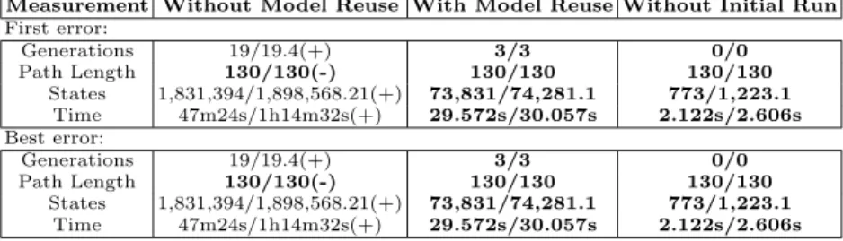
Table 3. Measurements from the model reuse runs on the Dining Philosophers 128 system
Measurement Without Model Reuse With Model Reuse Without Initial Run
First error: Generations 19/19.4(+) 3/3 0/0 Path Length 130/130(-) 130/130 130/130 States 1,831,394/1,898,568.21(+) 73,831/74,281.1 773/1,223.1 Time 47m24s/1h14m32s(+) 29.572s/30.057s 2.122s/2.606s Best error: Generations 19/19.4(+) 3/3 0/0 Path Length 130/130(-) 130/130 130/130 States 1,831,394/1,898,568.21(+) 73,831/74,281.1 773/1,223.1 Time 47m24s/1h14m32s(+) 29.572s/30.057s 2.122s/2.606s
The results in Table 3 show statistics for the Dining Philosopher problem family. In the Dining Philosopher system, there is a single error. The error can be reached in multiple ways but is always at the same depth/path length. This explains the similarity between the first and best results. From the numbers achieved, it is clear that model reuse can have a huge impact on the amount of computational effort required to find errors in the larger instance. The mean time
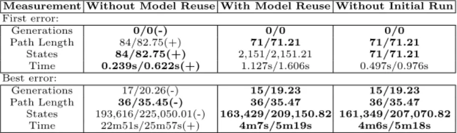
Table 4.Measurements from the model reuse runs on the Leader 10 system
Measurement Without Model Reuse With Model Reuse Without Initial Run
First error: Generations 0/0(-) 0/0 0/0 Path Length 84/82.75(+) 71/71.21 71/71.21 States 84/82.75(+) 2,151/2,151.21 71/71.21 Time 0.239s/0.622s(+) 1.127s/1.606s 0.497s/0.976s Best error: Generations 17/20.26(-) 15/19.23 15/19.23 Path Length 36/35.45(-) 36/35.47 36/35.47 States 193,616/225,050.01(-) 163,429/209,150.82 161,349/207,070.82 Time 22m51s/25m57s(+) 4m7s/5m19s 4m6s/5m18s
Table 5.Measurements from the model reuse runs on the GIOP 20 system
Measurement Without Model Reuse With Model Reuse Without Initial Run
First error: Generations 0/0.01(+) 17/17 0/0 Path Length 132/150.09(+) 61/73.37 61/73.37 States 40,421/60,681.01(+) 90,773/98,194.14 10,295/17,716.14 Time 1m26s/2m1s(+) 3m28s/3m46s 19.56s/38.017s Best error: Generations 30/28.71(+) 20/28.21 3/11.21 Path Length 31/31.21+) 26/25.6 26/25.6 States 13,068,139/12,337,306(+)1,495,644/4,942,260.07 1,415,166/4,861,782.07 Time 6h47m16s/8h13m24s(+) 57m34s/3h12m14s 54m26s/3h9m6s
to discover an error is reduced by over 99%. This means that rather than wait an hour for additional information regarding the error, information can be obtained in a mere 30 seconds, potentially reducing time spent in the debugging cycle substantially in this case. We expected a large gain on the Dining Philosopher family as it is a symmetrical problem. The strategy to finding an error in the Dining Philosopher is trivial, “Always choose the action that is Pickup the Left Fork”.
The results in Table 4 show statistics for the Leader election problem family. In this problem family, the results are less impressive than that of the Dining Philosopher family. We attribute this to the fact that the EDA can find a short counterexample with little computation, often in the first generation before any strategy building has taken place. This suggests that the model is trivial and does not require mechanisms to reduce computational effort. However, we still obtain a significant speed increase in terms of time spent searching the transition system. We attribute this to the EDA exploring a narrower area of the state space on the larger instance due to the initial strategy constructed from the smaller instance. This may avoid expanding useless parts of the search space, resulting in a reduction in CPU and memory usage.
The most impressive results are listed in Table 5 for the GIOP problem family. We expected poorer results on this model due to the description of the system being asymmetric. However, not only is a 62% reduction of mean time in finding a best error achieved (86% reduction in the median time), the quality of the solutions discovered are also improved. The improvement in the path length of the solutions found allow a practitioner to instantly assess the properties of the error. In this instance, the paths are of a similar length meaning it is highly
likely that only a subset of the processes in the system are required to cause the error. If all 20 clients were involved, you can expect a substantial increase in the path length over the 2 client model. The Dining Philosopher system, for instance, requires that all processes perform actions to cause a deadlock, and this is reflected by the increase in path length from the 32 philosopher system to the 128 philosopher system. Model reuse and the ability of the EDA to find and optimise counterexamples efficiently [11,12] could make the EDA-based technique a valuable tool for practitioners, as useful information such as this could be revealed along with other insights. Furthermore, the practitioner could gain this information with zero effort, as there is the potential for this approach to be automated.
5
Conclusion
To summarise, we have presented an approach for saving computational and manual effort when building and debugging concurrent systems using the EDA-based technique described in [11,12]. This is achieved by reusing information, specifically information from the models constructed, from an earlier execution to aid the search in a future execution. The analysis and reuse of modelling information learned by EDAs is an often cited advantage [8], and we have used this advantage in a practical scenario. Using this new approach, we have shown that it is possible to save computational effort when analysing problem fami-lies, and described other scenarios where effort could potentially be saved. Our results show that information can been gained using an insignificant amount of additional computational resources. This information can yield insights that can save time in the debugging phase, which could ultimately lower development costs. The scenario we have tested in this paper could potentially be automated, meaning no manual effort would be required to gain additional information. At the time of writing, we believe that this is the first application of EDA model analysis/reuse in the SBSE domain.
We believe that there is ample scope for further work in this area. The sce-narios for model reuse described and tested in this work are likely a subset of what is possible. There may well be other scenarios in which this work could be beneficial, and not just in the concurrent software testing domain. N-gram GP is essentially a sequence modelling algorithm, and approaches like this could be used wherever the solution space can be represented as a sequence. This could include problems that can be couched as graph search. We feel that the EDA de-scribed in [11,12] can be applied to stress testing. In this application domain, the EDA could be used to learn problematic sequences that cause the performance of systems to degrade or indeed completely fail. Augmenting the sequence mod-elling used in our work is another potential avenue of future research. We have previously outlined a number of ways in which N-gram GP can be improved to further increase efficiency when tackling large problems [11]. Using an entirely different sequence modelling approach may also increase the efficacy of the EDA in the concurrent software testing domain.
Acknowledgments. This work is supported by an EPSRC grant (EP/ D050618/1), SEBASE: Software Engineering By Automated SEarch.
References
1. Alba, E., Chicano, F.: Finding safety errors with ACO. In: Proceedings of the 9th Annual Conference on Genetic and Evolutionary Computation, pp. 1066–1073. ACM Press, New York (2007)
2. Alba, E., Chicano, F.: Searching for liveness property violations in concurrent systems with ACO. In: Proceedings of the 10th Annual Conference on Genetic and Evolutionary Computation, pp. 1727–1734. ACM, New York (2008)
3. Alba, E., Chicano, F., Ferreira, M., Gomez-Pulido, J.: Finding deadlocks in large concurrent java programs using genetic algorithms. In: Proceedings of the 10th Annual Conference on Genetic and Evolutionary Computation, pp. 1735–1742. ACM, New York (2008)
4. Clarke, E.M., Grumberg, O., Peled, D.A.: Model Checking. The MIT Press, Cam-bridge (2000)
5. Edelkamp, S., Lafuente, A.L., Leue, S.: Directed explicit model checking with HSF-SPIN. In: Proceedings of the 8th International SPIN Workshop on Model Checking of Software, pp. 57–79. Springer-Verlag New York, Inc., New York (2001)
6. Edelkamp, S., Leue, S., Lluch-Lafuente, A.: Protocol verification with heuristic search. In: AAAI-Spring Symposium on Model-based Validation Intelligence, pp. 75–83 (2001)
7. Luke, S., Panait, L., Balan, G., et al.: Ecj 16: A java-based evolutionary computa-tion research system (2007)
8. Pelikan, M., Goldberg, D.E., Lobo, F.G.: A survey of optimization by building and using probabilistic models. Computational Optimization and Applications 21(1), 5–20 (2002)
9. Poli, R., McPhee, N.F.: A linear estimation-of-distribution GP system. In: O’Neill, M., Vanneschi, L., Gustafson, S., Esparcia Alc´azar, A.I., De Falco, I., Della Cioppa, A., Tarantino, E. (eds.) EuroGP 2008. LNCS, vol. 4971, pp. 206–217. Springer, Heidelberg (2008)
10. Russell, S.J., Norvig, P., Canny, J.F., Malik, J., Edwards, D.D.: Artificial intelli-gence: a modern approach. Prentice hall, Englewood Cliffs (1995)
11. Staunton, J., Clark, J.A.: Searching for safety violations using estimation of distri-bution algorithms. In: IEEE International Conference on Software Testing, Verifi-cation, and Validation Workshop, pp. 212–221 (2010)
12. Staunton, S., Clark, J.A.: Finding short counterexamples in promela models using estimation of distribution algorithms. To appear: Search-based Software Engineer-ing Track, Genetic and Evolutionary Computation Conference (2011)