ISSUES IN MINING SURVEY DATA
A Project Report
Submitted to the Department of Computer Science In Partial Fulfillment of the Requirements
for the Degree of Master of Science
in
Computer Science University of Regina
By
Syed Uzair Ahmed Bahelvi Regina, Saskatchewan
May 4, 2005
c
Abstract
A survey is a system for collecting information from or about people to describe, compare, or explain their knowledge, attitudes, and behavior. Today, billions of dollars are spent annually collecting survey data, and surveys are everywhere. The extensive use of surveys has lead to collection of huge amount of survey data. This massive amount of data is not of much use unless and until it is analyzed and some useful knowledge is extracted from it. For decades, statistics has been used as a tool for analyzing survey data. Hence, survey data are usually collected and recorded in a format suitable for statistical analysis. Recently, data mining has emerged as an active field for analyzing data. This has led the survey data organizers to record data in a format helpful for data miners. Great care is taken while collecting and recording data, but still there remain a few problems for data miners. In this project we present a few problems faced while mining survey data for association rules and present a solution to solve that problem.
The purpose of a survey can range from describing some phenomenon, to establish-ing some relationships between variables. In this project, we concentrate on bivariate associations, that is, to see whether two variables are associated. We show how crosstabulations, a bivariate analysis technique can be used to determine bivariate associations. We show that the same information can be obtained from association
mining. We then show how association mining becomes more advantageous than crosstabulations as the number of variables for bivariate analysis increase.
Acknowledgments
I would like to express my sincere thanks to my supervisor, Dr. Robert Hilderman for his advice, assistance and financial support. Without his encouragement this work would not have been accomplished. I would also like to thank the Faculty of Graduate Studies and Research, and Department of Computer Science for financial support, my friends and relatives for their moral support, and my parents for making me capable of doing this type of work. Finally, I would like to thank my brother, and my sister.
Post Acknowledgments
I would also like to thank the internal examiners, Dr. Samira Sadaoui and Dr. Lisa Fan for their valuable comments and suggestions on my project report.
Contents
Abstract i
Acknowledgments iii
Post Acknowledgments iv
Table of Contents v
List of Tables viii
List of Figures x
Chapter 1 Introduction 1
1.1 Overview of Knowledge Discovery in Databases . . . 2
1.2 Overview of Surveys . . . 4
1.3 Overview of Survey Data Analysis . . . 6
1.4 Objectives of the Project . . . 7
1.5 Contributions of the Project . . . 7
1.6 Organization of the Project Report . . . 8
2.1 Overview of Association Rule Mining . . . 11
2.2 Key Issues of Surveys . . . 16
2.2.1 Purposes of Surveys . . . 17
2.2.2 Types of Surveys . . . 17
2.2.3 Designs of Surveys . . . 18
2.2.4 Sample Selection in a Survey . . . 19
2.2.5 Type of Information Collected in a Survey . . . 19
2.2.6 Survey Data Processing . . . 19
2.2.7 Types of Variables in a Survey . . . 22
2.2.8 Noise in Survey Data . . . 23
2.3 Conclusion of the Chapter . . . 24
Chapter 3 Data Preparation for Association Rule Mining 25 3.1 Features of the CCHS Data . . . 26
3.2 Survey Data Mining Problems . . . 29
3.3 PreAssociation Algorithm . . . 30
3.4 PreAssociation Software . . . 32
3.4.1 Block Diagram of PreAssociation Software . . . 34
3.4.2 Features of PreAssociation Software . . . 39
3.5 IBM’s Intelligent Data Miner . . . 41
3.6 Conclusion of the Chapter . . . 42
Chapter 4 Crosstabulations and Association Rules 44 4.1 Overview of Crosstabulations . . . 44
4.1.2 Interpreting a Crosstabulation . . . 47 4.2 Crosstabulations Vs Association Rules . . . 48 4.3 Conclusion of the Chapter . . . 50
Chapter 5 Experimental Results 51
5.1 Crosstabulations Method to find Associations . . . 52 5.2 Association Mining Method to find Associations . . . 52 5.3 Interrelation between Crosstabulations and Association Rules . . . . 54 5.4 Comparison between Crosstabulations and Association Mining . . . . 56 5.5 Conclusion of the Chapter . . . 59
List of Tables
2.1 An Example Survey Dataset . . . 12
2.2 Variables contained in the Example Survey Dataset and the Associated Domain Values . . . 13
3.1 Survey Data in the Raw Format . . . 26
3.2 Description of the Survey Data Variables . . . 27
3.3 Description of the Survey Data Variable Values . . . 28
3.4 Survey Data in Market Basket Format . . . 32
3.5 Full Form of PreAssociation Block Diagram Labels . . . 34
4.1 A simple Crosstabulation . . . 45
4.2 Crosstabulation with Row, Column and Total Percentages . . . 46
5.1 Crosstabulation for Sex versus HDI . . . 52
5.2 Association Rules for Sex and HDI . . . 53
5.3 Correspondence between Association Rules and Crosstabulations-Part1 56 5.4 Correspondence between Association Rules and Crosstabulations-Part2 57 5.5 Crosstabulation for Sex versus HDI . . . 58
5.6 Crosstabulation for Sex versus ToD . . . 58
5.7 Crosstabulation for HDI versus ToD . . . 59
List of Figures
1.1 KDD Process . . . 3
3.1 PreAssociation Algorithm . . . 30
3.2 Block Diagram of PreAssociation Software . . . 33
3.3 File Breaker . . . 36
3.4 Data File Tracker . . . 37
3.5 Data Reader . . . 38
3.6 Description Reader . . . 39
3.7 Print Market Basket . . . 40
Chapter 1
Introduction
Recently, data mining has been recognized as a key research topic by many re-searchers and as a powerful data analysis tool in many application areas. One such application is survey data analysis. For decades, statistical tools have remained as the only tools and techniques for survey data analysis. For this reason, survey data are usually created and recorded in a format suitable for statistical analysis. But recent trend of data mining has set the survey data organizers to create data suitable for data miners. Though a lot of care is taken while collecting and recording survey data, there still exist a few issues for data miners. Overcoming such issues is one of the steps of knowledge discovery in databases. In this chapter we present an introduction to knowledge discovery in databases, survey data and survey data analysis.
In Section 1.1, we present an overview of knowledge discovery in databases. Sec-tion 1.2 presents an overview of surveys. SecSec-tion 1.3 presents an overview of survey data analysis and then presents the various factors that affect the survey data analy-sis and the stepwise procedure of survey data analyanaly-sis. In Section 1.4, we present the objective of our project and in Section 1.5 the contributions of our project are
report.
1.1
Overview of Knowledge Discovery in Databases
Data mining, which is also referred to as Knowledge Discovery in Databases (KDD), is defined as a nontrivial process of identifying valid, novel, potentially useful, and understandable patterns in data [20, 25, 10]. Heredataimplies a set of facts (for example, records in a database) and patterns implies some form of an expression in some language describing a small subset of the data. Nontrivial implies that KDD is not a simple computation process, rather it involves some search or inference. The term process implies that KDD is comprised of many steps. Valid implies that the discovered patterns should be valid on new data with some degree of certainty and the term novel implies that the discovered knowledge should not be obvious, that is, the discovered knowledge should be some new information, not already known. Poten-tially usefulimplies that the KDD process should provide some benefit to the user or the system, that is, should help solve some problem or provide some useful knowledge or direction. Finally understandableimplies that the results obtained should be easy for human interpretation.
As shown in Figure 1.1, KDD is an iterative process that consists of a number of steps. Some of the commonly used steps [20, 12, 19, 10] are as follows:
• The goal identification step necessitates understanding of the application do-main, the relevant prior knowledge and then identification of the goal of the KDD process from the user’s point of view.
Patterns Transformed Preprocessed Data Data Target Data Data - - - - - - - - Selection Preprocessing Transformation Data Mining Interpretation/ Evaluation Knowledge Figure 1.1: KDD Process
records and/or data variables that will be mined.
• The data cleaning and preprocessing step includes removal of noise (unwanted or erroneous data), gathering information pertaining to noise, and strategies to handle missing data.
• The data reduction and transformation step reduces the volume of the data through dimensionality reduction and transformations to find invariant repre-sentations of the data.
• Thedata mining step specifies the data mining algorithm to be used for discov-ering patterns and generate a particular representational form such as clusters, classification trees, or association rules.
• The interpretation and evaluation step involves visualization of the discovered patterns and verification of these patterns against the expected results.
• The application step applies the newly discovered and verified knowledge to some problem domain, such as to decision making process or to cross verify the knowledge obtained from some other system.
The steps of the knowledge discovery process are interdependent. That is, the task to be performed in a certain step depends to some extent on the task to be performed in some other step. For example, given a database D, if we decide to extract the knowledge from D in the form of association rules (which can be related to the goal identification step), then the task to be performed in data mining step is association mining. If not already available in the required format, the data transformation step has to transform D into the format required for association mining.
1.2
Overview of Surveys
A survey is a system for collecting information from or about people to describe, compare, or explain their knowledge, attitudes, and behavior [3, 11, 2, 6]. Today, billions of dollars are spent annually collecting survey data, and surveys are every-where. Surveys are now commonly used by both public and private organizations to collect information. Governments, political parties, private corporations, trade unions, community groups, health researches and university researchers are all prime users of survey knowledge. The extensive use of surveys has lead to collection of huge amount of survey data. This massive amount of data is not of much use unless and until it is analyzed and some useful knowledge is extracted from it.
The routine of survey data analysis may not be difficult, but properly to guide it and the accompanying interpretation requires a familiarity with the background of
the survey and with all its stages [11]. Some of the key issues of surveys to become familiar with are as follows [11, 9, 2]:
• The purpose of a survey can range from describing some phenomenon, to es-tablishing relationships between variables, to providing information about what changes can be introduced to produce a desired change in something else.
• Thesample populationis a subset of population treated as representative of the entire population.
• The types of survey which are divided based on the medium through which they are conducted such as (a) mail or postal surveys (b) group-administered or hand-delivered questionnaires (c) face-to-face interviews and (d) telephone interviews.
• The survey design includes longitudinal design, experimental design and cross-sectional design, depending upon the time in which the measurements of the sample population are taken.
• Thetype of informationcollected largely depends upon the purpose of the survey and the industry conducting the survey. The information ranges from lifestyle habits, to households, to participation in election.
• The data processing is the final step of the survey system and the first step towards analyzing survey data. In this step, the answers from the survey re-spondents are translated and transferred into a computerized data file.
1.3
Overview of Survey Data Analysis
Once the data have been collected they are analyzed to get some useful informa-tion. There are three factors that affect on how the data are analyzed [4] including the number of variables being examined (one variable, two variables, and three or more variables), the level of measurement of the variables (nominal, ordinal, and interval/ratio), and the purpose of data analysis (descriptive or inferential).
Depending upon the above three factors, the process of data analysis can be defined stepwise as follows [4]:
• Determine the number of variables in question.
• Depending upon the number of variables, choose the appropriate method of analysis, that is:
– One variable→ Univariate analysis – Two variables →Bivariate analysis – Three variables → Multivariate analysis
• Depending upon the level of measurement of variables, choose an appropriate univariate, bivariate or multivariate technique. Following are some of the sur-vey data analysis techniques.
– Univariate→ Frequency distributions
– Bivariate→ Crosstabulations, Scattergrams, Regression, Rank order correla-tion, Comparison of means
– Multivariate → Conditional tables, Partial rank order correlation, Multiple and partial correlation, Multiple and partial regression, Path analysis
• Depending upon the data analysis technique, choose an appropriate descriptive statistics and an appropriate inferential statistics, if required.
1.4
Objectives of the Project
The objectives of this project are:
• To prepare survey data for generating human interpretable association rules and
• To show that the same information can be obtained from association mining as from crosstabulations, and to show that association mining is advantageous over crosstabulations as the number of variables for bivariate analysis increase.
Realizing this objective consists of two steps:
• To preprocess survey data for association mining.
• To generate association rules, crosstabulations on survey data and compare them.
1.5
Contributions of the Project
This project makes the following contributions to the field of survey data analysis:
• We develop and implement an algorithm to preprocess the survey data for as-sociation mining and also address the data selection step of the KDD process. While doing so, we discuss the various issues pertaining to the format in which
the survey data is typically collected and recorded. The survey data is not pro-vided in the format required for association mining. Therefore, before associa-tion mining funcassocia-tion could be applied, the survey data needs to be preprocessed and transformed to the required format.
• We generate the association rules and build crosstabulations on the survey data and compare them. We theoretically show that the same information can be obtained from the association rules as obtained from the crosstabulations. We show that bivariate associations between n variables can be obtained in just one run of the association mining compared to building n×(n-1)/2 crosstabulations. We then run the experiments to validate our point.
1.6
Organization of the Project Report
The remainder of this report is organized as follows. In Chapter 2, we present the general overview of association rule mining and highlight its characteristics. We then present an overview of the key issues of surveys that are required for survey data analysis.
In Chapter 3, we present the problem faced while generating association rules from survey data. we develop and implement an algorithm to preprocess the survey data for association mining. We then present the functions of our software components and highlight the features of our software. Using IBM’s Intelligent Data Miner [8], we show how to generate association rules from the preprocessed survey data.
In Chapter 4, we present an overview of crosstabulations and show how the as-sociation rules correspond to the information given by crosstabulations. We then
theoretically describe how the association rules are advantageous over crosstabula-tions as the number of variables being examined increase.
In Chapter 5, we present and discuss the experimental results to validate our theoretical justifications.
Chapter 2
Background
In surveys, the information is collected from a sample of people who have been selected to represent a larger population and the resulting information is then gen-eralized back to the larger population. In this way, three types of knowledge can be gained from surveys [11]: (a) accurate description of how attitudes and behaviors are distributed in the population, (b) analysis of the associations among attitudes and behaviors, and (c) clues to cause and effect relationships. To obtain the required knowledge from a survey, the data collected in the survey has to be processed and analyzed using an appropriate technique. Association rule mining is a data mining technique used to find the associations between various items in the given data. The association rules reveal the existing dependencies in the data, that is, the presence of one item or a collection of items implies the presence of some other item or a collec-tion of items. This in turn gives us a deeper insight of the data and helps us make better decisions.
In Section 2.1, we present an overview of association rule mining by reviewing the significant previous work done in this area [14, 23, 1]. In Section 2.2, we present an overview of the key issues of surveys that are important for survey data analysis.
2.1
Overview of Association Rule Mining
In this section, we present the formal definition of association mining, the descrip-tion of the associadescrip-tion rule support, the descripdescrip-tion of the associadescrip-tion rule confidence, and the description of the association rule lift.
• Problem Definition: Formally, association mining has been defined as follows
[14, 23, 1, 10, 18, 24]: Let I = i1, i2, .,im be a set of m distinct literals, called items. Let D be a set of transactions, where each transaction T is a set of items such that T⊂I. A transaction T is said to contain X if and only if X⊂T. An association rule is an implication of the form X→Y, where X⊂I, Y⊂I, and X∩Y = Ø. X is called the antecedent or rule body and Y is called the consequent or rule head of the rule. The rule body expresses the condition that must be satisfied for the rule head to become true. A set of items (such as rule body or the rule head) is called an itemset. So, an association rule also expresses associations between itemsets. The association rule X→Y has support s in transaction set D if s% of transactions in D contain X∪Y. The rule X→Y holds with confidence c in transaction set D if c% of transactions in D that contain X also contain Y. In other words, the confidence of an association rule X→Y measures the conditional probability of Y given X, denoted by P(Y|X). Lift of an association rule is a value that gives us information about the increase in probability of the “then” (consequent) part given the “if” (antecedent) part, that is, lift gives us the information that helps us to determine whether the antecedent part of a rule (rule body) has a positive effect on the consequent part of the rule (rule head), has a negative impact or has no impact at all.
To give a better idea of the support, confidence and lift measures, we demonstrate them with the help of an example. Since the theme of this paper is to demonstrate the potential use of data mining on survey data, a sample survey database is used in the example instead of the typical “market basket” transactional database that is usually described in previous work [14, 23, 1]. Hence, the terminologies relevant to survey data will be used rather then those associated with transactional data. That is, an item will be referred to as a variable, an itemset as a variableset, a transaction as a record, and a TID (Transaction Identification Number) as a record number.
Record
Number SEX HDI NCC ToD
1 Male Excellent 0 Regular
2 Male Excellent 0 Regular
3 Female Good 2 Occasional
4 Male Very Good 1 Former
5 Female Good 2 Occasional
6 Male Good 1 Regular
7 Male Excellent 0 Former
8 Female Fair 3 Never
9 Female Good 2 Occasional
10 Female Poor 5+ Former
11 Female Poor 5+ Occasional
12 Male Fair 2 Former
13 Female Good 2 Never
14 Female Very Good 1 Regular
15 Female Fair 3 Former
Table 2.1: An Example Survey Dataset
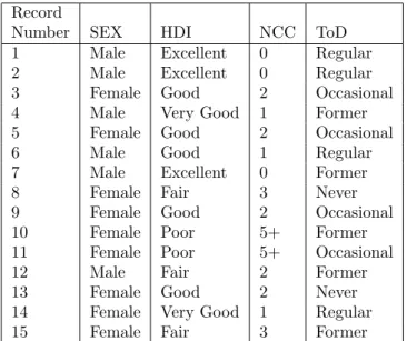
Consider the example survey dataset containing 15 records, shown in Ta-ble 2.1, representing a population health survey data. The Record Number variable contains the unique identification number given to each survey respon-dent. Each of the four remaining variables contains the responses to a series
HDI NCC ToD
SEX (Health Description (Number of (Type of
(Gender) Index) Chronic conditions) Drinker)
Male Excellent 0 Regular
Female Very Good 1 Occasional
Good 2 Former
Fair 3 Never
Poor 4
5+
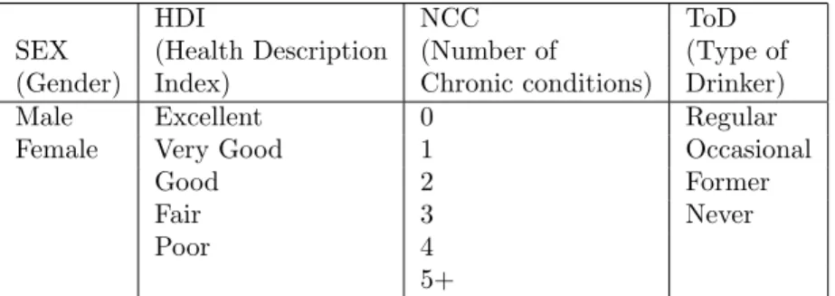
Table 2.2: Variables contained in the Example Survey Dataset and the Associated Domain Values
of survey questions for each respondent. For example, the SEX variable cor-responds to the query “What is your Gender”. Similarly the HDI (Health Description Index), NCC (Number of Chronic Conditions) and ToD (Type of Drinker) variables correspond to the queries “Which category would you con-sider to represent your health”, “How many chronic conditions do you exhibit” and “How often do you drink”, respectively. For example, the person identified by Record Number 3, is of ‘Female’ Sex, exhibits ‘Good’ Health Description Index, has ‘2’ Number of Chronic Conditions and is an ‘Occasional’ Type of Drinker.
Let I ={Sex, HDI, NCC, ToD} be a set of 4 variables. Let D ={records 1 to 15 of Table 1} be a set of records over I, where each record contains a set of variable values. For instance, in Table 2.1, the record 1 ={Male Sex, Excellent HDI, 0 NCC, Regular ToD}. Referring to records 1, 2 and 6 of Table 2.1, we obtain a rule saying “ifSex =Male then ToD = Regular”. This rule has only one variable in rule body (Sex =Male) and rule head (ToD =Regular) that can be represented as: Sex(Male) → ToD(Regular). Similarly, referring to records
1, 2, 3 and 9 of Table 2.1, we obtain the following association rules that have variableset in their rule head and/or rule body: Sex(Male) + HDI(Excellent)
→ToD(Regular),Sex(Female) + HDI(Good) → NCC(2) + ToD(Occasional). The number of variables in the rule body and rule head together form the length of the association rule. Hence, in the above three rules, the first one is of length 2, the second rule is of length 3 and third rule is of length 4.
• Rule Support: Each variableset I, in a set of records D, has an associated
measure of statistical significance called support [25, 23, 1]. For a variableset X⊂I, support can be represented as support(X) = s, if the fraction of records in D containing X iss. That is,support(X) is the number of records containing variableset X divided by the total number of records. For example, from Ta-ble 2.1, support for the variaTa-bleset “(Sex(Male) + HDI(Excellent))” is 3/15 = 0.2 or 20%, which comes from records numbered 1,2 and 7. This can also be represented assupport(Sex(Male) +HDI(Excellent)) = 20%.
In a given set of records, the support of a given rule is always equal to the support of the variableset that consists of the variables in the rule body and the variables in the rule head of the rule. For instance, the support for the rule “Sex (Male) + HDI (Excellent) → ToD (Regular)” is equal to the support for the variableset “Sex (Male) + HDI (Excellent) + ToD (Regular)”.
• Rule Confidence: A given rule has a measure of its strength called the
con-fidence [25, 23, 1]. The rule X → Y in the transaction set D has confidence c represented as,conf(X →Y), ifc% of the transactions in D that contain X also contains Y. For example, from Table 2.1, conf(Sex (Male) + HDI (Excellent)
→ToD (Regular)) = 2/3 = 0.66 or 66%.
Confidence can also be calculated as conf(X → Y) = support(X ∩ Y)/ support(X). It is often desirable to concentrate on rules with high values of support and confidence. Such rules with strong support and high confidence are called as strong rules [23].
• Rule Lift: Lift is the ratio of confidence to expected confidence [13, 15] and expected confidence can be understood as follows: If two variablesets X and Y are statistically independent, the support for records containing both the vari-ablesets X and Y is equal to the product of the support for variableset X and the support for variableset Y. i.e.,support(X∩Y) =support(X)×support(Y). The confidence obtained for such records containing statistically independent variablesets is called expected confidence. From the definition of confidence, we have conf(X→Y) = support(X∩Y)/support(X). Further, assuming statis-tical independence, expected confidence can be written as exp conf(X→Y) = support(X)×support(Y)/support(X) = support(Y). In other words, expected confidence means, “confidence, if the presence of variableset X does not enhance the presence of variableset Y”, which according to the above equation is equal to the support of the variableset Y.
Now, lift can be defined as the factor by which confidence exceeds expected confidence, that is,lift(X→Y)=conf(X→Y)/exp conf(X→Y)=conf(X→Y)/ support(Y). For example, referring to records 1 and 2 of Table 2.1, we have
lift(Sex(Male)+HDI(Excellent)→ToD(Regular)) =conf(Sex(Male)+HDI(Excellent)
association between variables or variablesets, that is, a high lift value indicates a positive relation between the rule head and the rule body. A lift value less than one is considered low and indicates a negative relation between rule head and rule body and lift value of one is considered neutral. Thus the above rule tells us that Male Sex and Excellent HDI has a positive effect on the person being aRegular ToD, that is, if a person is ofMale Sex andExcellent HDI then it is very likely for the person to be a Regular TOD because the lift value is greater than one.
2.2
Key Issues of Surveys
Once the survey data has been collected it has to be analyzed. To properly guide the survey data analysis process, we have to be familiar with the background of the survey and with all its stages [11]. In this section, we briefly present the key issues of surveys [9, 2, 5] .
In Section 2.2.1, we present a few common purposes of surveys. In Section 2.2.2, we present the various types of survey. In Section 2.2.3, we present the different designs of surveys. In Section 2.2.4, we present the advantages of sample selection in a survey. In Section 2.2.5, we briefly present the type of information collected in a survey. In Section 2.2.6, we present the processing of data after surveys are conducted. In Section 2.2.7, we present the types of variables in survey data. In Section 2.2.8, we define noise and briefly present how noise gets collected in a survey data.
2.2.1
Purposes of Surveys
There are many purposes for which a survey is conducted. Some of the common ones are as follows [11]:
• To describe some phenomenon.
• To establish some relationships between variables.
• To describe how attitudes and behaviors are distributed in the population.
• To analyze the associations among attitudes and behaviors.
• To find the clues to cause and effect relationships.
2.2.2
Types of Surveys
Survey respondents can provide answers either orally or in writing. Oral responses come in interviews that can be conducted either in person or over the telephone. Written responses come from self-administered questionnaires that are distributed either through the mail or by delivery. Survey research involves either direct, per-sonal contact with respondents or indirect, less perper-sonal contact. Interviews pro-vide for a two-way exchange of information and thus the closest contact. In con-trast, self-administered questionnaires are impersonal since they allow no dialogue be-tween respondents and researchers. Based on the medium through which the surveys are conducted they have been divided as [9]:(a) Mail or postal surveys (b) Group-administered or Hand-delivered questionnaires (c) Face-to-Face interviews and (d) Telephone interviews.
2.2.3
Designs of Surveys
The three important designs of surveys can be found in [9, 4], including:
• Longitudinal: Designs where measurements are taken at multiple times are
referred to as longitudinal designs. A longitudinal survey involves surveying the same group of people over a longer period of time. This allows us to track trends in population health. These powerful designs help in pinpointing causal influences because we can see how variables change together over time.
• Experimental: In experimental designs a group of individuals are randomly
assigned to either the experimental group or the control group. After grouping, the measurements for dependent variable, which is the same in both the groups, are taken from both the groups. Then the independent variable is activated only for experimental group and the measurements for dependent variable are again taken from both the groups. Finally, the measurements for dependent vari-able taken from both the groups before and after the activation of independent variable are compared. This method provides an effective way of ensuring the change in dependent variable caused by independent variable.
• Cross Sectional: Designs where measurements are taken at one single point
in time are referred to as cross-sectional designs. These designs can be likened to single snapshots from a camera, as compared to a continuous longitudinal view provided by a motion picture.
2.2.4
Sample Selection in a Survey
It would be very expensive, and not very practical, to survey every person in a Country. Collecting information from a sample is more economical than collecting information from an entire population [4]. Sampling, a statistical method, is an established way to determine the characteristics of an entire population using the answers from a randomly chosen sample. The information obtained by surveying a sample population may actually be more satisfactory than that obtained by surveying the entire population. For various reasons, errors occur in data collection. They are more likely to occur when available resources are spread more thinly among more numerous survey units. Consequently, these errors are more likely to occur when enumerating a population than a sample because the former is more numerous than the later.
2.2.5
Type of Information Collected in a Survey
The type of information collected in surveys is very diverse. Some of the topics of information are [11]: population, housing, community studies, family life, sexual be-havior, family expenditure, nutrition, health, education, social mobility, occupations and special groups, leisure, travel, political behavior, race relations and minority groups, old age, crime and deviant behavior.
2.2.6
Survey Data Processing
Once all the questionnaires have been returned or all the interviews completed, the work of analyzing the results begin. A first step in this process is to transfer
Using the data file that results from the coding process, the survey can then be systematically analyzed [9]. All the information necessary to read and understand the data file is provided. The reader knows the name of the variable. In case where the variable name is not sufficient informative for readers, an extended variable name or variable label is given. Values and their labels also appear in the table. If some respondents did not answer the questions or the questions did not apply to them, the number of missing cases is listed.
In Section 2.2.6.1, we present a description on how the information collected from the survey is coded and transferred to the computer data files. In Section 2.2.6.2, we present the format in which survey data typically collected and recorded.
2.2.6.1 Coding the Survey Data
Coding involves transferring the survey information to computer data files. The codes are the values used to represent different responses. For statistical analysis, numeric representations or codes are used for each values of every variable. For ex-ample, if the respondent answers “male” to the question, “what is your gender?” a number such as “0” is chosen to represent male survey respondents. A different num-ber, such as “1” is then assigned to female survey respondents. In case of computer assisted questionnaires or interviews, the coding scheme is developed as part of the questionnaire. Responses are directly and automatically entered into the computer database.
2.2.6.2 Format of Survey Data
While creating the codebook for survey data, each of survey respondent receives an identification number (ID) to differentiate from other survey respondents. The responses to each question (variable) will be coded by assigning a numeric value for each possible response, with all the responses making up a data line. In turn, all the data lines will make up a data set or data matrix. A data line could look like 01 2 23 1 0 10 6 or like 0122310106, with each number representing the value of a variable, as in 01 (ID), 2 (female), 23 (age) and so on.
1. Fixed format: The computer must be instructed on exactly how to read the
data line. For example, the computer is instructed to read column 1 and 2 together as one number; to skip column 3; read column 4 as one number, etc. The number of the digits to be read as one number is referred to as field width, while the left-hand column where the computer starts reading is referred to as the field location. Note that the value “1”, when entered into a field two columns wide is written as “01”, or “1”, with the space preceding the digit 1 representing a blank (known as right justification). The above process is referred to as fixed format because the location of each variable in the data line is fixed. For each variable, then, the computer reads the number in each data line to determine its value.
A completed codebook for fixed format survey data contains the following in-formation [9]:
• Question number (or Identification number): This makes it clear to locate the information.
• Variable name: Each variable name must be unique and usually short names starting with alphabetic character are used.
• Variable label: These are longer character strings clarifying the precise meaning of the shorter variable name.
• Value label: This identifies each category or value of a variable.
• Variable value: A number that stands for or represents each value a vari-able takes on.
• Field width: This identifies how many values the variable can take on.
• Field location or column location: This identifies the column in which the values for a particular variable start.
2. Free format: Data that are entered in free format have the variable values
entered in a consistent sequence for all cases, but the specific field location is not fixed. Each code in this case is separated by a space or a comma. In the case of free format, the codebook would require neither the field location nor the field width.
2.2.7
Types of Variables in a Survey
In a survey there are two types of variables [21], such as:
1. Direct Variables: If the value of a variable is collected directly from the response of the survey respondent, then such a variable is called direct variable.
2. Derived Variables: If the value of a variable is derived from the values of direct variables, then such a variable is called derived variable.
2.2.8
Noise in Survey Data
We define noise as the data values that appear in the data as a result of, unan-swered queries or queries that are not relevant to the survey respondent. These are the values that we do not want to appear in our results.
There are various instances through which noise gets collected in the survey data. We show here two common contexts in which noise gets collected in the survey data, by considering variable values ‘Not Applicable’ and ‘Not Stated’ as noise.
• Noise through direct variables: If the survey respondent does not respond to a direct variable, then its value is recorded as ‘Not Stated’. If a variable is designed specific to the people of a certain region, then the value of that variable is recorded as ‘Not Applicable’ for the people of the other regions. For example, if a variable is designed specific to the people of Saskatchewan, then the value of such variable for the people of Ontario is recorded as ‘Not Applicable’.
• Noise through derived variables: If the value of a derived variable is highly dependent on the particular value‘v’ of a direct variable, then the value of the derived variable becomes ‘Not Applicable’ for any value of the direct variable other than ‘v’. For example, Consider that the value of “Type of Drinker” variable is derived from two variables “Frequency of drinking” and “Ever Had a drink?”. Also consider that the value of “Type of Drinker” variable is highly dependent on the value of “Ever had a drink?” variable. If the value of that variable is ‘No’ or ‘Not Stated’ , then the value of the “Type of Drinker” variable becomes ‘Not Applicable’ or ‘Not Stated’, respectively.
2.3
Conclusion of the Chapter
In this chapter, we presented an overview of association rule mining and high-lighted its parameters. We then presented an overview of surveys and highhigh-lighted the key issues of surveys required for survey data analysis.
Chapter 3
Data Preparation for Association Rule
Mining
For decades, statistics has been used as a tool for analyzing survey data. Hence, survey data are usually collected and recorded in a format suitable for statistical analysis. Recently, data mining has emerged as an active field for analyzing data. This has led the survey data organizers to record data in a format helpful for data miners. Though high care is taken while collecting and recording data, there remain a few problems for data miners. In this chapter we present the problems faced while mining survey data for association rules and present a solution.
In Section 3.1, we present how survey data are typically recorded using CCHS data as an example. In Section 3.2, we present the problems faced while generating association rules from survey data and propose a solution to the problem. In Sec-tion 3.3, we develop an algorithm, which we name as PreAssociaSec-tion algorithm, to preprocess survey data for association mining. In Section 3.4, we present the func-tions and features of the PreAssociation software, which is an implementation of the PreAssociation algorithm.
3.1
Features of the CCHS Data
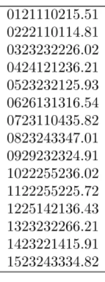
The CCHS is a cross-sectional survey that collects information related to health status, health care utilization and health determinants for the Canadian population [21]. The CCHS operates on a two-year collection cycle, Cycle1.1 and Cycle 1.2. CCHS data that is recorded in the fixed format. The data file used in our exper-iments contains data collected in the first year of collection for the CCHS (Cycle 1.1). Information was collected between September 2000 and November 2001, for 136 health regions, covering all provinces and territories of Canada.
0121110215.51 0222110114.81 0323232226.02 0424121236.21 0523232125.93 0626131316.54 0723110435.82 0823243347.01 0929232324.91 1022255236.02 1122255225.72 1225142136.43 1323232266.21 1423221415.91 1523243334.82
Table 3.1: Survey Data in the Raw Format
The CCHS data has 614 data variables and 130800 records. It is stored in a matrix format with 614 columns, each column corresponding to a data variable and 130800 rows, each row corresponding to a data record, as a typical survey data is stored. Each record corresponds to the responses of an individual survey respondent to all the 614 data variables (questions). The data file is available in various formats,
Variable Name Length Position Variable Description
XYZ1 2 1-2 Record Number
XYZ2 2 3-4 Province
XYZ3 1 5-5 SEX
XYZ4 1 6-6 Health Description Index
XYZ5 1 7-7 Number of Chronic Conditions
XYZ6 1 8-8 Type of Smoker
XYZ7 1 9-9 Type of Drinker
XYZ8 3 10-13 Height
XYZ9 1 14-14 Standard Weight
Table 3.2: Description of the Survey Data Variables
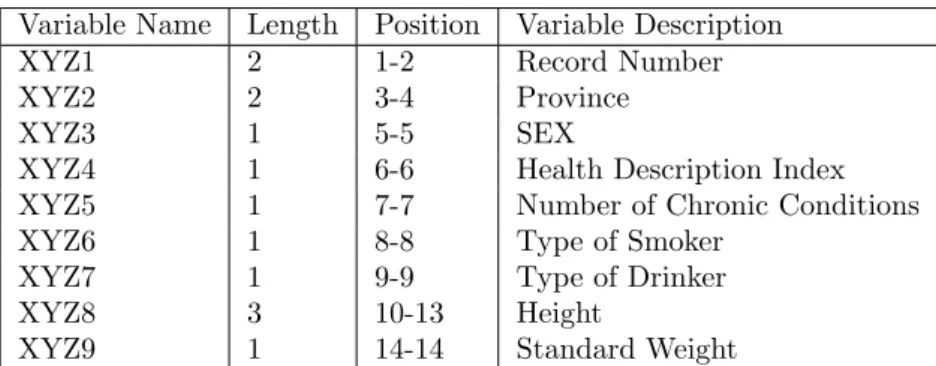
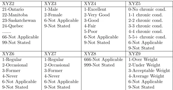
saved with the extensions .sav, .dat, .txt, etc. We have used the .txt file for our experiments. Table 3.1 shows the raw format in which the CCHS data is stored, an encoded text file, by considering a few variables from the CCHS data. Note that the data file has no delimiters that makes it difficult to differentiate between different variables. Also, the data is stored in numeric codes, which makes it difficult to interpret their meaning. Therefore, a separate file is provided to give the details of the data variables. Table 3.2 shows the details of how the data file shown in Table 3.1 is encoded, that is, the variable name, the length of the variable (the number of digits or the number of columns corresponding to the variable), the position of the variable (the column corresponding to the start position of the variable) and the description of the short variable name. For example, the XYZ4 variable has length one, that is, it is represented by one digit in the data file of Table 3.1, is stored in column 6 and stands for Health Description Index. Table 3.3 shows the associated variable values and gives the description of the numeric values. For example, XYZ4 variable has 7 associated numeric values. The description of the numeric values for XYZ4 is also shown in Table 3.3.
XYZ2 XYZ3 XYZ4 XYZ5
21-Ontario 1-Male 1-Excellent 0-No chronic cond.
22-Manitoba 2-Female 2-Very Good 1-1 chronic cond.
23-Saskatchewan 6-Not Applicable 3-Good 2-2 chronic cond.
24-Quebec 9-Not Stated 4-Fair 3-3 chronic cond.
... 5-Poor 4-4 chronic cond.
66-Not Applicable 6-Not Applicable 5-5+ chronic cond.
99-Not Stated 9-Not Stated 6-Not Applicable
9-Not Stated
XYZ6 XYZ7 XYZ8 XYZ9
1-Regular 1-Regular 666-Not Applicable 1-Over Weight
2-Occasional 2-Occasional 999-Not Stated 2-Under Weight
3-Former 3-Former 3-Acceptable Weight
4-Never 4-Never 4-Average Weight
6-Not Applicable 6-Not Applicable 6-Not Applicable
9-Not Stated 9-Not Stated 9-Not Stated
Table 3.3: Description of the Survey Data Variable Values
be read as follows: The survey respondent with record number 01, is from Ontario province, is of male sex, has excellent health description index, exhibit no chronic conditions, is an occasional type of smoker, is a regular type of drinker, has 5.5 feet of height, and isover weight.
Of the 614 variables in the CCHS data, some are direct variables and some are derived variables. By direct variable, we mean that the value of that variable is the direct response of the survey respondent to the questionnaire corresponding to that variable. For example the XYZ4 is a direct variable corresponding to the question “Which category would you consider to represent your health”, provided with cate-gories. By derived variable, we mean that the value of that variable is derived from the values of other direct variables. For example the XYZ7 variable is a derived vari-able derived from the values of the direct varivari-able like “Ever had a drink”, “Frequency of drinking alcohol”, “ Number of drinks at a time” etc.
3.2
Survey Data Mining Problems
While generating association rules from raw survey data, we face a couple of problems, including:
• Uncomprehensible Association Rules: As shown in Section 3.1, survey data is recorded in an ASCII encoded text file. If we apply association mining on it, we will obtain the association rules like:
1→ 2 0 + 1→ 2.
These association rules makes no sense because we cannot figure out which variable they are referring to and hence what value they represent.
• Noise in Survey Data : As explained in Section 2.2.8, a lot of noise gets accu-mulated in survey data and hence if association mining is applied on such data many rules will be generated with noise in their rule body and/or rule head.
To overcome the problem faced while generating association rules from survey data, we seek the following solution, that is, preprocess survey data such that:
• Human interpretable association rules are generated.
• Noise is eliminated before the application of the association mining.
In the following sections, we show how we try to achieve the goal of generating noise free and human interpretable association rules.
PreAssociation Algorithm
1. begin
2. D = {input data file} 3. I = {data description file} 4. O = {output data file} 5. V = {selected data variables} 6. R = {selected data records} 7. for each data record r ∈ R 8. begin
9. for each data variable v ∈ V 10. begin
11. a = read the numerical value for ‘v’ from D 12. if (a ≠Noise)
13. begin
14. d1 = retrieve the description for ‘a’ from I 15. d2 = retrieve the description for 'v' from I 16. print (r, d1+ d2) to O in market basket format 17. end;
18. end; 19. end; 20. end;
Figure 3.1: PreAssociation Algorithm
3.3
PreAssociation Algorithm
Figure 3.1 shows the PreAssociation algorithm developed to preprocess the survey data for association mining. Lines 2 through 6 specify the user inputs to the algorithm. In line 2, the user specifies the input data file D, that is, the file containing survey data in raw format. In line 3, the user specifies the data description file I, that is, the file containing the variable position, variable length, variable description and variable value description. In line 4, the user specifies the output file O, that is, the file in which the preprocessed survey data will be stored. In line 5, the user specifies the particular data variables to be used for preprocessing (hence use for association mining after preprocessing) among the total number of data variables. In line 6, the
user specifies the particular data records to be preprocessed (hence use for association mining after preprocessing) among the total number of data records. Line 7 selects a data recordr, to be preprocessed, from the data file D and loops through lines 8 to 19 until all the data records r ∈ R are preprocessed. The preprocessing of the selected data recordr starts from line 8. Line 9 selects a data variable v, to be preprocessed, from the selected data record r and loops through lines 10 to 18 until all the data variables v ∈ V are preprocessed. The preprocessing of the selected data variables starts from line 10. Line 11 reads the ascii data value,a, for the selected data variable v from the input data file D. Line 12 checks if the data value a is a noise or not. If a is a noise, then preprocessing for that data value stops and the line 9 loops to read the next variable value. If a is not a noise, then lines 13 through 17 are executed. Lines 14 and 15 retrieve the descriptions fora and v from the data description file I. Line 16 prints the descriptions fora andv along with r, in the market basket format, to the output data file O. We explain the algorithm shown in Figure 3.1 in detail by running over the example survey dataset of Table 3.1 that has been built using a few variables and the format of CCHS dataset.
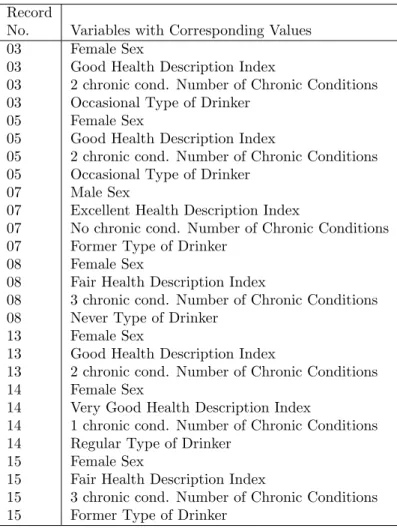
Consider the dataset shown in Table 3.1 as the input data file, D, to the Pre-Association Algorithm. Consider for example selected data variables V = {XYZ3, XYZ4, XYZ5, XYZ7} and selected data records R = {XYZ2 = 23}. Let us also consider Noise ={Not Applicable}. Then after the application of the Pre-Association algorithm to the above data files, we obtain the output data file, O, as shown in the Table 3.4.
If we have a closer look at the output data file above, the variable ’Type of Drinker’ is missing from the record number 13. The reason is that in record number 13, the
Record
No. Variables with Corresponding Values
03 Female Sex
03 Good Health Description Index
03 2 chronic cond. Number of Chronic Conditions
03 Occasional Type of Drinker
05 Female Sex
05 Good Health Description Index
05 2 chronic cond. Number of Chronic Conditions
05 Occasional Type of Drinker
07 Male Sex
07 Excellent Health Description Index
07 No chronic cond. Number of Chronic Conditions
07 Former Type of Drinker
08 Female Sex
08 Fair Health Description Index
08 3 chronic cond. Number of Chronic Conditions
08 Never Type of Drinker
13 Female Sex
13 Good Health Description Index
13 2 chronic cond. Number of Chronic Conditions
14 Female Sex
14 Very Good Health Description Index
14 1 chronic cond. Number of Chronic Conditions
14 Regular Type of Drinker
15 Female Sex
15 Fair Health Description Index
15 3 chronic cond. Number of Chronic Conditions
15 Former Type of Drinker
Table 3.4: Survey Data in Market Basket Format
variable ’Type of Drinker’ has ’Not Applicable’ as its value (coded as 6 in input data file), which we consider as unwanted value or noise in our data file and hence get eliminated from the output data file.
3.4
PreAssociation Software
In this section we present the implementation of the PreAssociation algorithm and name it as PreAssociation software, which preprocesses a given survey data for
PreAssociation Processor IDF SVI N ODF SDR DDF File Breaker Data Reader Data File Tracker Description Reader Print PreAssociation Format VLF VDF vDF SVI SDR N VVD VPF CRN CVI PreAssociation Processor NDV DDF IDF ODF
Figure 3.2: Block Diagram of PreAssociation Software
association mining.
In Section 3.4.1, we present the block diagram of the PreAssociation software and show how its various components function together. In Section 3.4.2, we present the features of the PreAssociation software.
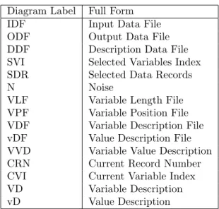
Diagram Label Full Form
IDF Input Data File
ODF Output Data File
DDF Description Data File
SVI Selected Variables Index
SDR Selected Data Records
N Noise
VLF Variable Length File
VPF Variable Position File
VDF Variable Description File
vDF Value Description File
VVD Variable Value Description
CRN Current Record Number
CVI Current Variable Index
VD Variable Description
vD Value Description
Table 3.5: Full Form of PreAssociation Block Diagram Labels
3.4.1
Block Diagram of PreAssociation Software
Figure 3.2 shows the block diagram of the PreAssociation software. Due to space problem, short notations are used to label the block diagram. The full forms of the short notations are given in Table 3.5.
3.4.1.1 Input to PreAssociation Software
The PreAssociation software takes the following five inputs:
1. Input data file (IDF) containing survey data in raw format.
2. Data description file (DDF) describing the input data file.
3. Indexes of the selected data variables (SVI)(a manual list is created to represent all the survey data variables by indexes as shown in Figure 3.4).
4. Selected data records (SDR) that specify the number of records to be pre-processed out of the total number of records and the particular records to be preprocessed. The particular records are selected by, first selecting one or more data variables and then selecting a particular category of that variable/s. For example, we can first select the Sex variable and then select Male category in the Sex variable to preprocess the records with only Male Sex.
5. Noise(N) through which we can specify the unwanted values in the preprocessed survey data and hence the unwanted values in the association rules.
3.4.1.2 Components of PreAssociation Software
The PreAssociation software consists of five components, including:
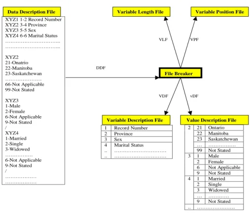
1. File Breaker:
The function of the File Breaker is to break the Data Description File into subfiles. As shown in Figure 3.3, the File Breaker component takes the Data Description File (DDF) as input and breaks it into four different files, that is, Variable Length File (VLF) that contains the lengths of all the data variables in the input data file. Variable Position File (VPF) that contains the starting position of all the data variables in the input data file. Variable Description File (VDF) that contains the descriptions of all the data variables. Value Description File (vDF) that contains the descriptions of the values of all the data variables.
2. Data File Tracker:
XYZ1 1-2 Record Number XYZ2 3-4 Province XYZ3 5-5 Sex XYZ4 6-6 Marital Status ……….. ……….. XYZ2 21-Onatrio 22-Manitoba 23-Saskatchewan ……… 66-Not Applicable 99-Not Stated XYZ3 1-Male 2-Female 6-Not Applicable 9-Not Stated / XYZ4 1-Married 2-Single 3-Widowed ………. 6-Not Applicable 9-Not Stated / ……… ……… 1 Record Number 2 Province 3 Sex 4 .. .. Marital Status ……… ……… 21 Ontario 22 Manitoba 23 Saskatchewan … ………. 2 99 Not Stated 1 Male 2 Female 6 Not Applicable 3 9 Not Stated 1 Married 2 Single 3 Widowed … ………… 4 9 Not Stated .. ………. Variable Description File
Variable Position File Variable Length File
Value Description File Data Description File
File Breaker
DDF
VLF VPF
VDF vDF
Figure 3.3: File Breaker
record has to be read from the Input Data File for processing in the current operation. As shown in Figure 3.4, the Data File Tracker component takes the Input Data File, the Selected Variables Index (SVI), and the Selected Data Records as input and provides the Current Record Number (CRN) andCurrent Variable Index (CVI) as output.
3. Data Reader: The function of the Data Reader is to read the data from
the Input Data File from the specified location, that is, specified record and specified variable in that record.
0000012322…. 0000022111…. 0000032312…. ………. ………. 1308002321…. Province = 23 Total < = 120500 ……… 2 3 4 .. 523
Input Data File
Selected Variables Index Data File Tracker
Selected Data Records
Current Record = Previous Record + 1
Is Current Record Selected?
N Y
Get Next Variable Index
Current Record Number Current Variable Index
3 2
Get Next Record
Y
Figure 3.4: Data File Tracker
(IDF), the Variable Length File (VLF), the Variable Position File (VPF), the Current Record Number (CRN), and theCurrent Variable Index (CVI) as input and provides theAscii Data Value (ADV) as output.
4. Description Reader:
The function of the Description Reader is to retrieve the descriptions for the given variable and the given variable value from the given DataDescription File (DDF).
As shown in Figure 3.6, the Description Reader component takes the Variable Description File (VDF), theValue Description File (vDF), the Noise (N), the
0000012322…. 0000022111…. 0000032312…. ………. ………. 1308002321…. 1 6 2 2 3 1 4 1 .. .. 1 1 2 7 3 9 4 10 .. ..
Input Data File Variable Length File Variable Position File
Data Reader Current Variable Index Current Record Number 3 2 3 2 2 2 2 7 3, 7, 2 23 23
Ascii Data Value
23
Figure 3.5: Data Reader
Current Variable Index (CVI), and the Ascii Data Value (ADV) as input and providesVariable Value Description (VVD) as output.
5. Print Market Basket: The function of the Print Market Basket is to print
the preprocessed survey data in the market basket format.
As shown in Figure 3.7, thePrint Market Basket component takes the Current Record Number (CRN) and theVariable Value Description (VVD) as input and prints them to the Output Data File (ODF) in market basket format.
1 Record Number 2 Province 3 Sex 4 .. .. Marital Status ……… ……… 21 Ontario 22 Manitoba 23 Saskatchewan … ………. 2 99 Not Stated 1 Male 2 Female 6 Not Applicable 3 9 Not Stated 1 Married 2 Single 3 Widowed … ………… 4 9 Not Stated .. ……….
Variable Description File Value Description File
Ascii Data Value
23
Current Variable Index
2 Description Reader 2 2 2, 23 Saskatchewan Province
Variable Value Description
Saskatchewan Province Noise Not Applicable, Not Stated Check if data value is noise
Figure 3.6: Description Reader
3.4.2
Features of PreAssociation Software
In this section we walk through the features available in our software PreAssoci-ation. PreAssociation is implemented in C language on Unix platform.
The PreAssociation software converts the given survey data from survey-format to PreAssociation-format, without which it would not be possible to generate meaning-ful association rules from survey data. Following are some of the helpmeaning-ful features availed by our software:
• The software allows us to select any number of records and any particular records out of the total number of records available. This helps us select a part
000001 Saskatchewan Province 000001 Female Sex 000001 Single Marital Status ……… ……… 000003 Saskatchewan Province 000003 Male Sex
000003 Single Marital Status ……… ……… ……… ……… 120490 Saskatchewan Province 120490 Female Sex 120490 Married Marital Status ……… ………
Output Data File Variable Value Description
Saskatchewan Province
Current Record Number
3
Print Market Basket Format
Saskatchewan Province
3
3, Saskatchewan Province
Figure 3.7: Print Market Basket
• The software gives us the option to select any number of variables of our choice among the total variables available to perform association mining on them. This helps us to concentrate and generate association rules of only those variables, which we are concerned about rather than generating thousands of rules consist-ing of all the variables, makconsist-ing it hard to interpret the results. But at the same time, the program also allows us to select all the variables available depending on our choice and need.
For example, as it has been mentioned earlier, the CCHS was conducted over entire Canada and data was collected from all the provinces and territories. These provinces were in turn divided into various health regions. Taking this point into consideration, we have designed the software such that, it avails us with the option of selecting the data for association mining from any particular province and the program also gives us the option of selecting any particular health region from within that province. This helps us to concentrate on any
sub section of the data and generate rules on it. It also helps us to do a com-parative study at different levels of data. For example, we can compare the rules generated for different health regions within the same province or we can do a comparison at provincial level by comparing the rules generated for dif-ferent provinces. The program also allows us to select all the data records for preprocessing.
• Another feature availed by our software helps us to get rid of the unwanted values (or noise) in the data, without deleting the whole record containing that unwanted value as done by SPSS, a statistic software. By eliminating just the unwanted value and not the entire record containing it, we retain the other valuable information present in that record.
3.5
IBM’s Intelligent Data Miner
In this chapter, we briefly present the tutorial on IBM’s Intelligent Data Miner, a data mining tool and show how to generate the association rules from the Pre-Association data file. Due to the limited space available, we explain only the impor-tant and essential steps.
The process of KDD using the Intelligent Miner include the following steps [8]:
• Create the data object by selecting the input data file.
• Transform the data by reorganizing it, eliminating duplicate records, or con-verting it from one form to another (unfortunately there is no option for trans-forming the survey data for association mining).
• Run the data mining function.
• Visualize and analyze the resulting data.
We now generate association rules from preprocessed survey data using the Intel-ligent Data Miner. We use CCHS dataset as our input data file. For demonstration, we choose the following 4 variables: Sex, Type of Drinker, Health Description Index and Number of Chronic Conditions. We preprocess the CCHS data for the above 4 variables and transform it into PreAssociation format which serves as the input data file for association mining.
From the preprocessed survey data, the two columns, that is the Record Numbers and the Variables with corresponding values become input data fields for Intelligent Miner. Then we have to run the data miner to generate the human interpretable association rules as shown in Figure 3.8.
3.6
Conclusion of the Chapter
In this chapter, we presented the problems faced while generating association rules from survey data. We then presented the algorithm and the software developed to preprocess the survey data for association mining. We also presented the functions of our software components and highlight the features of our software. Using IBM’s Intelligent Data Miner [8], we showed how to generate association rules from the preprocessed survey data.
Chapter 4
Crosstabulations and Association Rules
Bivariate analysis is a statistical data analysis method used to see whether two variables are associated [4]. Two variables are said to be associated when the distri-bution of values on one variable differs for different values of the other. In statistics there are various techniques used for bivariate analysis. The most common one is crosstabulations. In this chapter, we compare crosstabulations with association rules and show how association rules correspond to the information given by the crosstab-ulations. We then show that as the number of variables increase, bivariate analysis through assocation mining is simpler than crosstabulations.
In Section 4.1, we present an overview of crosstabulations. In Section 4.2, we procide a theoretical justification to show the interrelation between crosstbulations and association rules.
4.1
Overview of Crosstabulations
Crosstabulations are a way of displaying data so that we can detect association between two variables [4].
In Section 4.1.1, we present the structure of a crosstabulation. In Section 4.1.2, we present how to interpret a crosstabulation.
4.1.1
The Structure of a Crosstabulation
Sex
Male Female Totals
Regular 3 1 4
Type of Occasional 0 4 4 Drinker Former 3 2 5
Never 0 2 2
Totals 6 9 15
Table 4.1: A simple Crosstabulation
In Table 4.1 there are two variables: Sex across the top and Type of Drinker on the side, having two and four categories respectively. There are two columns (one for each category of the top variable) and four rows (for each category of Type of Drinker). Tables can be described by their size which is represented as number of columns by number of rows. Thus Table 4.1 is a two by four table. There are three sets of totals: those on the side are called row totals (4, 4, 5, 2) since they represent the total number of people in that row. Those on the bottom (6, 9) are column total since they represent the number of people in that column. The number in the bottom right-hand corner (15) is the grand total.
Each column is broken into subgroups according to people’s characteristics on the other variable. Thus the Female column is broken down into four groups: female regular type of drinker, female occasional type of drinker, female former type of drinker and female never type of drinker. Each of these subcategories is called a cell.
The numbers in each cell represent the cell frequency or count.
To easily interpret the associations, the cell frequencies can be converted into percentages. A percentage is calculated by seeing what proportion of the total a particular number represents. But since we have three totals, depending on which total is used we get a different percentage with a different interpretation. For example, let us consider the top right hand cell(1) of Table 4.1, representing female regular type of drinkers, and convert its raw numbers into percentages.
Sex
Male Female Totals
Regular row% 75% 25% 100% column% 50% 11.1% 26.7% total% 20% 6.7% 26.7% Occasional row% 0% 100% 100% Type column% 0% 44.4% 26.7% of total% 0% 26.7% 26.7% Drinker Former row% 60% 40% 100% column% 50% 22.2% 33.3% total% 20% 13.3% 33.3% Never row% 0% 100% 100% column% 0% 22.2% 13.3% total% 0% 13.3% 13.3% Totals row% 40% 60% 100% column% 100% 100% 100% total% 40% 60% 100%
Table 4.2: Crosstabulation with Row, Column and Total Percentages
• The column total will produce a column percentage( column%). Using this we get 1/9 × 100 = 11.1%. This means 11.1% of the females are regular type of drinkers. It does not mean that 11.1% of regular type of drinkers are females.
= 25%. This means that 25% of regular type of drinkers are females.
• The grand total will produce a total percentage( total%). This gives us 1/15
× 100 = 6.7%. This means 6.7% of the whole population sample were female regular type of drinkers.
Table 4.2 shows the crosstabulation with row%, column% and total% after con-version of the cell frequencies of Table 4.1 into percentages.
4.1.2
Interpreting a Crosstabulation
A crosstabulation arranged as in Table 4.2 becomes very difficult to be read. We must decide which percentage to use. When trying to find the associations in the table, total% is of no value. We then have to choose between row% and column%. This choice depends on two things: first, on the way the table is arranged; second, depending on which variable is treated as independent and which as dependent. Once we have decided on the independent and dependent variable, the association between them can be detected by comparing their subgroups or categories. If the categories of the independent variable differ in terms of their characteristics on the dependent variable, then we can say they are associated; if there is no difference then they are not associated.
The process of detecting association in a crosstabulation can be defined as follows [4]:
1. Determine which variable to be treated as independent and which as dependent.
3. Compare percentages for each category of the independent variable within one category of the dependent variable at a time. Thus
• If the independent variable is across the top, use column% and compare these across the table. Any difference between these reflects some associ-ation.
• If the independent variable is on the side use row% and compare these down the table.
In general, we represent the row% or column% as %within the independent vari-able.
4.2