Air Force Institute of Technology
AFIT Scholar
Theses and Dissertations Student Graduate Works
3-21-2013
Automatic Modulation Classification of Common
Communication and Pulse Compression Radar
Waveforms using Cyclic Features
John A . Hadjis
Follow this and additional works at:https://scholar.afit.edu/etd
Part of theSignal Processing Commons, and theSystems and Communications Commons
This Thesis is brought to you for free and open access by the Student Graduate Works at AFIT Scholar. It has been accepted for inclusion in Theses and
Dissertations by an authorized administrator of AFIT Scholar. For more information, please [email protected].
Recommended Citation
Hadjis, John A ., "Automatic Modulation Classification of Common Communication and Pulse Compression Radar Waveforms using Cyclic Features" (2013).Theses and Dissertations. 870.
AUTOMATIC MODULATION CLASSIFICATION OF COMMON COMMUNICATION AND PULSE COMPRESSION RADAR
WAVEFORMS USING CYCLIC FEATURES
THESIS
John A. Hadjis, Second Lieutenant, USAF AFIT-ENG-13-M-20
DEPARTMENT OF THE AIR FORCE AIR UNIVERSITY
AIR FORCE INSTITUTE OF TECHNOLOGY
Wright-Patterson Air Force Base, Ohio
DISTRIBUTION STATEMENT A.
The views expressed in this thesis are those of the author and do not reflect the official policy or position of the United States Air Force, the Department of Defense, or the United States Government.
This material is declared a work of the U.S. Government and is not subject to copyright protection in the United States.
AFIT-ENG-13-M-20
AUTOMATIC MODULATION CLASSIFICATION OF COMMON COMMUNICATION AND PULSE COMPRESSION RADAR
WAVEFORMS USING CYCLIC FEATURES
THESIS
Presented to the Faculty
Department of Electrical and Computer Engineering Graduate School of Engineering and Management
Air Force Institute of Technology Air University
Air Education and Training Command in Partial Fulfillment of the Requirements for the Degree of Master of Science in Electrical Engineering
John A. Hadjis, B.S.E.E. Second Lieutenant, USAF
March 2013
DISTRIBUTION STATEMENT A.
AFIT-ENG-13-M-20
Abstract
This research develops a feature-based maximum a posteriori (MAP) classification system and applies it to classify several common pulse compression radar and communi-cation modulations. All signal parameters are treated as unknown to the classifier system except SNR and the signal carrier frequency. The features are derived from estimated duty cycle, cyclic spectral correlation, and cyclic cumulants. The modulations considered in this research are BPSK, QPSK, 16-QAM, 64-QAM, 8-PSK, and 16-PSK communication modulations, as well as Barker5 coded, Barker11 coded, Barker5,11 coded, Frank49 coded,
Px49coded, and LFM pulse compression modulations. Simulations show that average
cor-rect signal modulation type classification %C > 90% is achieved for SNR> 9dB, average signal modulation family classification %C > 90% is achieved for SNR> 1dB, and an av-erage communication versus pulse compression radar modulation classification %C >90% is achieved for SNR > −4dB. Also, it is shown that the classification performance using selected input features is sensitive to signal bandwidth but not to carrier frequency. Mis-matched bandwidth between training and testing signals caused degraded classification of %C ≈ 10%−14% over the simulated SNR range.
For my Family and Friends who listened to my research ramblings and helped me get through the stressful days
Table of Contents
Page
Abstract . . . iv
Dedication . . . v
Table of Contents . . . vi
List of Figures . . . viii
List of Tables . . . x
List of Acronyms . . . xi
I. Introduction . . . 1
1.1 Research Motivation and Related Research . . . 1
1.2 Research Goal . . . 2
1.3 Research Methodology . . . 3
1.4 Thesis Organization . . . 4
II. Literature Review . . . 5
2.1 Waveforms Considered . . . 5
2.1.1 Communication . . . 5
2.1.2 Radar . . . 8
2.2 Pattern Recognition . . . 15
2.2.1 Likelihood-Based Tests . . . 15
2.2.2 Feature Based Tests . . . 16
2.3 Cyclostationarity . . . 16
2.3.1 Theory . . . 18
2.3.2 Cyclic Autocorrelation Function . . . 19
2.3.3 Spectral Correlation Function . . . 22
2.4 Estimating the Spectral Correlation Function . . . 23
2.4.1 Temporal Smoothing . . . 25
2.4.1.1 FFT Accumulation Method . . . 28
2.4.1.2 Strip Spectral Correlation Algorithm . . . 30
2.4.2 Frequency Smoothing . . . 31
Page
III. Methodology . . . 36
3.1 Simulating Modulations . . . 36
3.2 Simulating SNR with AWGN . . . 41
3.3 Extracting Features . . . 43
3.3.1 Duty Cycle . . . 43
3.3.2 Cyclic Spectral Correlation . . . 45
3.3.3 Cyclic Cumulants . . . 50
3.4 Classifier Training . . . 52
3.5 Performance Criteria . . . 55
IV. Results and Analysis . . . 58
4.1 Simulation Setup . . . 58
4.2 Classifier Performance with Ideal Training Data . . . 60
4.2.1 Signal Modulation Type Classification . . . 60
4.2.2 Signal Modulation Family Classification . . . 65
4.2.3 Communication vs. Pulse Compression Radar Modulation Classi-fication . . . 69
4.3 Classifier Bandwidth Sensitivity . . . 73
4.4 Classifier Carrier Frequency Sensitivity . . . 76
V. Conclusions . . . 77
5.1 Summary . . . 77
5.2 Impact . . . 78
5.3 Recommendations for Future Work . . . 79
List of Figures
Figure Page
2.1 Communication Constellations . . . 7
2.2 Pulse Repetition Interval . . . 10
2.3 Nested Barker4,5Code . . . 14
2.4 Frequency Spectrum of Frequency Translates . . . 21
2.5 SCF Support Region . . . 23
2.6 Temporal Smoothing . . . 27
2.7 FAM Estimate Resolution . . . 29
2.8 SSCA Estimate Resolution . . . 30
2.9 Frequency Smoothing . . . 32
3.1 Waveform Simulation Process . . . 37
3.2 MATLAB® Generated Pulse Shaping Filter Properties . . . 39
3.3 MATLAB® Generated Pulse Shaping Filter Applied to Simulated BPSK Signal 40 3.4 Simulated SNR Scaling Process . . . 41
3.5 Estimating the Duty Cycle in Observation Time∆t . . . 44
3.6 Estimated Duty Cycles Over a Range of SNRdBwith 95% Confidence Intervals 45 3.7 Estimated BPSK SCF at SNR= 20dB . . . 46
3.8 Estimated QPSK SCF at SNR= 20dB . . . 47
3.9 Estimated BPSK SCF at SNR= −5dB . . . 48
3.10 Estimated SCF Feature Ratio . . . 50
3.11 Estimated Cyclic Cumulant Spectrums for BPSK . . . 51
3.12 Classifier Training . . . 54
3.13 Test the Classifier . . . 55
Figure Page 3.15 ROC Curve Examples . . . 57 4.1 Classifier System’s Average Performance for 12 Signal Modulation Types with
Ideal Training Data . . . 61 4.2 Classifier System’s Modulation Type Classification Performance with Ideal
Training Data . . . 62 4.3 Classifier System ROCs for 12 Modulation Types at SNR =9dB . . . 63 4.4 Classifier System ROCs for 12 Modulation Types at SNR =0dB . . . 64 4.5 Classifier System’s Average Performance for 7 Modulation Families with Ideal
Training Data . . . 66 4.6 Classifier System’s Modulation Family Classification Performance with Ideal
Training Data . . . 67 4.7 Classifier System ROCs for 7 Modulation Families at SNR =0dB . . . 68 4.8 Classifier System’s Average Performance for Distinguishing Communication
from Pulsed Radar Modulations with Ideal Training Data . . . 69 4.9 Classifier System’s Pulsed Radar and Communication Modulation
Classifica-tion Performance with Ideal Training Data . . . 70 4.10 Classifier System ROCs for Communication vs Pulsed Radar Detection at
SNR=−5dB . . . 71 4.11 Classifier System’s Performance Sensitivity to Bandwidth . . . 73 4.12 Classifier System’s Modulation Type Classification Performance with
Mis-matched Bandwidth . . . 74 4.13 Classifier System ROCs for 12 Modulation Types at SNR = 8dB with
Mismatched Bandwidth . . . 75 4.14 Classifier System’s Performance Sensitivity to Carrier Frequency . . . 76
List of Tables
Table Page
2.1 Known Barker codes [21] . . . 13
2.2 Some Frank Code Phase Sequences [21] . . . 14
2.3 Some Px Code Phase Sequences [21] . . . 14
2.4 Cumulant Partitions forn=4,q=2 . . . 33
2.5 Cumulants . . . 34
3.1 SCF Classifier Features . . . 49
3.2 Cyclic Cumulant Features . . . 52
3.3 Classifier Features . . . 53
4.1 Classifier System’s Confusion Matrix for 12 Modulation Types at SNR= 9dB . 61 4.2 Classifier System’s Confusion Matrix for the 12 Modulation Types at SNR=0dB 64 4.3 Modulation Families . . . 65
4.4 Classifier System’s Confusion Matrix for 7 Modulation Families at SNR=0dB 68 4.5 Radar and Communication Waveforms . . . 70
4.6 Classifier System’s Confusion Matrix for Communication vs Pulsed Radar Modulations at SNR =−1dB . . . 72
4.7 Classifier System’s Confusion Matrix for Communication vs Pulsed Radar Modulations at SNR =−5dB . . . 72
4.8 Classifier System’s Confusion Matrix for 12 Modulations Types at SNR=8dB with Mismatched Bandwidths . . . 75
List of Acronyms
Acronym Definition
ALRT average likelihood ratio test
ASK amplitude shift keying
AWGN additive white gaussian noise BPSK binary phase shift keying CAF cyclic autocorrelation function
CC cyclic cumulant
CTC cyclic temporal cumulant
CTCF cyclic temporal cumulant function DFT discrete fourier transform
EW electronic warfare
FAM fast fourier transform (FFT) accumulation method FFT fast fourier transform
FSK frequency shift keying
GLRT generalized likelihood ratio test
IF intermediate frequency
LFM linear frequency modulation
MAP maximuma posteriori
MATLAB® matrix laboratory
ML maximun likelihood
OFDM orthogonal frequency division multiplexing PDF probability density function
PMF probability mass function PRI pulse repetition interval
Acronym Definition
PSD power spectral density
PSK phase shift keying
QAM quadrature amplitude modulation QPSK quadrature phase shift keying RADAR radio detection and ranging
RF radio frequency
ROC receiver operating characteristic SCF spectral correlation function
SDR software defined radio
SNR signal to noise ratio
SSCA strip spectral correlation algorithm
TCF temporal cumulant function
TMF temporal moment function
WSCS wide-sense cyclo-stationary
AUTOMATIC MODULATION CLASSIFICATION OF COMMON COMMUNICATION AND PULSE COMPRESSION RADAR
WAVEFORMS USING CYCLIC FEATURES
I. Introduction
T
hischapter summarizes the research presented in this thesis. Its motivation and goalsare explained, as well as the assumptions used to limit the problem’s scope. Last, the organization of information and results presented in this thesis are explained.
1.1 Research Motivation and Related Research
In this digital age, with increasing technology and decreasing electronic component size, many capabilities are being integrated into single complex systems. Also, the ever increasing need for higher data rates and larger bandwidths in the electromagnetic spectrum is demanding efficient, adaptive new methods to utilize the licensed and unlicensed spectrums. The difficult task of increasing spectrum usage while mitigating incurred interference between independent signals can benefit from automatic modulation recognition processes applied to non-cooperative signals of interest.
Cognitive radio technology with software defined radios (SDRs) is receiving much research interest as a potential solution for spectrum management problems because SDRs can adaptively change critical parameters of their receive and transmit operations to adjust to current channel conditions. Accurately sensing and extracting information about current spectrum usage is a key process for a cognitive radio system. In fact, many research papers are solely focused on spectrum sensing techniques for cognitive radios [2, 18, 29]. The increasing complexity of electromagnetic environments is also providing new challenges
for electronic warfare (EW). Spectrums are beginning to overlap and user transmissions are becoming more dynamic in time, frequency, and modulation. Improved sensing techniques of the electromagnetic spectrum is key for future communication and radar systems such as cognitive radios and cognitive radars.
Within spectrum sensing research, automatic modulation recognition has emerged as an important process in cognitive spectrum management and EW applications. Research has been conducted on automatic classification of both digital and analog modulations for at least two decades, and possible applications in cognitive radar and communication systems include threat recognition and analysis, communication interception/demodulation, effective adaptive jammer response, and communication/radar emitter identification [5, 23]. The research continues to trend towards larger modulation sets and more complicated channel environments with minimala priorisignal knowledge. In [30], the feasibility of providing automatic modulation recognition as an integrative technology for radar and communication signals based on features was investigated, but only a limited set of modulation types were simulated and varying signal to noise ratio (SNR) analysis was not provided. [30] is the only research found that addresses both radar and communication waveform modulation recognition. This area remains relatively unexplored and is the focus of this research. A large modulation set including both pulse compression radar and communication modulations is explored for modulation classification with minimal knowledgea prioriof critical received signal parameters.
1.2 Research Goal
The goal of my research is to advance the application of modulation classification presented in the literature by developing and simulating a reliable automatic modulation recognition system capable of discerning between a wide range of non-cooperative com-mon pulse compression radar and communication modulations. Simulated performance
and limitations of the developed system will be assessed over a wide range of received SNR and varying received signal parameters.
1.3 Research Methodology
First, a wide set of communication and pulse compression radar modulations are simulated with varying SNRs by adding additive white gaussian noise (AWGN). Then, promising distinguishing features are researched and chosen for use in a classifier system. The research is directed by the literature which documents successful feature-based classification methods. This thesis applies these research findings to develop and simulate a reliable modulation classification system for both common communication and pulse compression radar modulations.
In [5], a survey is provided of prior research for automatic communication modulation classification techniques. These techniques are organized by statistical-based and feature-based methods. Although statistical-feature-based techniques are theoretically optimal, they are practically inefficient due to computational complexity. Feature-based techniques using cyclic spectrum features and cumulants are shown to have performed well for varying sets of communication modulations and unknown parameters. These same parameters were also shown to perform well for radar waveform modulation recognition in [23], and [30] illustrated that the estimated duty cycle of a received waveform may be used to distinguish between pulsed radar (linear frequency modulation (LFM) and bi-phase barker5 coded)
and conventional communication (AM, FM, ASK, FSK, BPSK, QPSK) signals with 100% accuracy for SNR greater than 8dB.
The research performed in this thesis is focused on leveraging signal properties that have been shown to be successful modulation classification features to develop a versatile classifier system capable of reliably classifying the modulation of several common communication and radar modulated waveforms. These signal properties include signal duty cycle, cyclostationarity, and cyclic cumulant statistics which were researched for
classification feature selection to distinguish between binary phase shift keying (BPSK), quadrature phase shift keying (QPSK), 16-quadrature amplitude modulation (QAM), 64-QAM, 8-phase shift keying (PSK), and 16-PSK communication signals as well as bi-phase Barker5 coded, bi-phase Barker11 coded, bi-phase Barker5,11 coded, Frank49 coded, Px49
coded, and LFM pulse compression radar signals.
1.4 Thesis Organization
Chapter II introduces the basic theory of the communication and radar modulations considered, and describes the common classification methods currently utilized for modulation recognition. It then summarizes the theory found in literature concerning cyclostationarity and various algorithms to estimate the spectral correlation function (SCF). Last, the topic of cyclic cumulants (CCs) is addressed.
InChapter III, the steps taken to develop the modulation classification system based on the theory provided in Chapter II are presented. First, the process of simulating the various communication and radar waveforms is explained as well as the process used to simulate the received SNR. Then, the process of extracting the signal features researched in Chapter II and training the classifier algorithm is explained. Last, the criteria used to assess the developed modulation classification system’s performance are presented.
Chapter IV provides the classifier’s test simulation results as described in Chapter III. Figures for probability of correct classification over a wide SNR range, confusion matrices for SNRs of interest, and receiver operating characteristic (ROC) curves for SNRs of interest are presented for multiple test simulations with varying test parameters. These results are analyzed and compared to assess the classifier’s performance.
Finally, Chapter V gives a summary of the research with an estimate of its findings’ theoretical and operational impact. The thesis concludes with a discussion of potential areas for continued research and further testing.
II. Literature Review
T
hischapter provides a theoretical background of concepts used in this research as wellas a review of previous work published in the area of interest. Section 2.1 covers the various communications and radar waveforms considered in the research. Section 2.2 introduces the two main approaches to classification and pattern recognition. Section 2.3 provides the development of cyclostationary concepts such as the cyclic autocorrelation function (CAF) and spectral correlation function (SCF). These concepts are extended for practical applications by introducing various methods to estimate the cyclic spectrum of signals in Section 2.4. Last, Section 2.5 provides the framework for higher-order cyclic statistics as used in this work.
2.1 Waveforms Considered
This research includes a broad range of common communication and radar waveforms for modulation recognition analysis. This section presents the fundamental theory for defining each modulation type and provides the general equations that represent them.
2.1.1 Communication.
Digital forms of communication can vary envelope, phase, frequency, or any combination of these to relay information through radio frequency (RF) transmission. This information is generally encoded and represented with communication symbols. A modulation scheme utilizing Msymbols is referred to asM-ary. The simplest modulation forms only modulate in one domain and are well known as M-ary amplitude shift keying (ASK), M-ary phase shift keying (PSK), and M-ary frequency shift keying (FSK). M-ary quadrature amplitude modulation (QAM) is a form of modulation in which both amplitude and phase are varied to form communication symbols. In this research, binary phase shift keying (BPSK), quadrature phase shift keying (QPSK), 8-PSK, 16-PSK, 16-QAM, and
64-QAM communication modulations are considered. All theory in this section is derived from information found in [24, 26].
M-ary ASK transfers information through its amplitude where each amplitude level represents a communication symbol. Transmitted ASK symbols at a carrier frequency, fc,
fit the mathematical form
ASK : s(t)= Amcos (2πfct) 0≤t ≤Tsym (2.1)
whereAmis one of M distinct envelope amplitudes representing communication symbols.
In M-ary PSK, however, amplitude is constant because information is transferred through its carrier phase. The carrier phase may have one of M values in any symbol periodTsym
given by
θm =
2π
M (m−1) (2.2)
wherem=1,2,· · · ,M. Therefore, the modulatedM-PSK waveform at a carrier frequency is M-PSK : sm(t)= Acos 2πfct+ 2π M (m−1) ! (2.3) where 0 ≤ t ≤ Tsym and m = 1,2,· · · ,M. From Equation (2.3) we can calculate the
transmitted symbols for BPSK, QPSK, 8-PSK and 16-PSK:
BPSK : sm(t)=Acos (2πfct+mπ) m= 1,2 (2.4a) QPSK : sm(t)=Acos 2πfct+ π 2(m−1) m= 1,2,3,4 (2.4b) 8-PSK : sm(t)=Acos 2πfct+ π 4(m−1) m= 1,2,· · · ,8 (2.4c) 16-PSK : sm(t)=Acos 2πfct+ π 8(m−1) m= 1,2,· · · ,16 (2.4d) where 0 ≤ t ≤ Tsym. Utilizing the trig identity cos(A+ B) = cosAcosB− sinAsinB,
these transmitted signals can be represented in quadrature form with the basis functions φ1(t) = cos(2πfct) andφ2(t) = sin(2πfct). The signal constellations are shown in this two
)
(
1t
φ
)
(
1t
φ
φ
1(
t
)
)
(
1t
φ
)
(
1t
φ
)
(
2t
φ
)
(
2t
φ
φ
2(
t
)
)
(
2t
φ
)
(
2t
φ
)
(
1t
φ
(a) BPSK Constellations)
(
1t
φ
)
(
1t
φ
φ
1(
t
)
)
(
1t
φ
)
(
1t
φ
)
(
2t
φ
)
(
2t
φ
φ
2(
t
)
)
(
2t
φ
)
(
2t
φ
)
(
1t
φ
(b) QPSK Constellations)
(
1t
φ
)
(
1t
φ
φ
1(
t
)
)
(
1t
φ
)
(
1t
φ
)
(
2t
φ
)
(
2t
φ
φ
2(
t
)
)
(
2t
φ
)
(
2t
φ
)
(
1t
φ
(c) 8 PSK Constellations)
(
1t
φ
)
(
1t
φ
φ
1(
t
)
)
(
1t
φ
)
(
1t
φ
)
(
2t
φ
)
(
2t
φ
φ
2(
t
)
)
(
2t
φ
)
(
2t
φ
)
(
1t
φ
(d) 16 PSK Constellations ) ( 1 tφ
) ( 1 tφ
φ
1(t))
(
1t
φ
)
(
1t
φ
)
(
2t
φ
) ( 2 tφ
φ
2(t))
(
2t
φ
)
(
2t
φ
) ( 1 tφ
(e) 16 QAM Constellations
) ( 1t φ ) ( 1t φ φ1(t)
)
(
1t
φ
) ( 1 t φ ) ( 2 t φ ) ( 2 t φ φ2(t))
(
2t
φ
) ( 2 t φ ) ( 1t φ (f) 64 QAM Constellationsdimensional basis function space in Figure 2.1. Also, M-ary PSK signals have constant envelope magnitudes so the constellation points are equally spaced on a circle of radiusA
centered at the origin. The constellations for BPSK, QPSK, 8-PSK, and 16-PSK are shown in Figure 2.1a, Figure 2.1b, Figure 2.1c, and Figure 2.1d respectively.
Figure 2.1a illustrates that BPSK can be equal to 2 level antipodal binary ASK. For the case that its two phases are separated by 180◦, Equation (2.4a) for BPSK is equal
to Antipodal 2-ASK from Equation (2.1). For example, let the phase take the values θ=0 andπso that the transmitted BPSK signal is
sm(t)= Acos (2πfct+mπ) m= 1,2 (2.5a)
= ±Acos (2πfct) (2.5b)
It can be seen that although the phase is being shifted, the amplitude of the BPSK signal envelope can take the two values±Aas in ASK.
M-ary QAM varies both its carrier phase and envelope amplitude to represent data symbols. M-QAM modulated signals can be defined as
M-QAM : sm(t)= Amφ1(t)+Bmφ2(t), 0≤t ≤Tsym, m=1,2,· · · ,M (2.6)
whereφ1(t) = cos (2πfct),φ2(t) = sin (2πfct), Am andBmare defined as Am = (2am−1)−
√
M and Bm = (2bm−1) −
√
M with am and bm all combinations of integers in the set h
1,2,· · · , √Mi. For 16-QAM,AmandBmmay have values [−3,−1,1,3] and for 64-QAM,
AmandBmmay have values [−7,−5,−3,−1,1,3,5,7]. The constellations for 16-QAM and
64-QAM are therefore square lattices instead of circular and are shown in Figure 2.1e and Figure 2.1f respectively.
2.1.2 Radar.
RADAR stands for radio detection and ranging (RADAR) and it summarizes the two main tasks of RADAR systems. That is to detect targets and determine their range from the RADAR system [21]. The selection of a radar waveform and its specifications are
fundamental to the performance and capabilities of a radar system. Generally, the received signal energy determines the reliability of detection, but the specifications of the waveform are responsible for the accuracy, resolution, and ambiguity of range and Doppler (range rate) of the target [21]. Variables that may be manipulated in RADAR waveforms include: operating frequency, peak power, pulse duration, bandwidth, pulse repetition interval (PRI), modulation type/coding, and polarization. In general, continuous wave RADAR has very good Doppler sensitivities but weak range resolution. Pulsed RADAR is very versatile and, depending on design, can have good radar resolution in Doppler and range estimates to provide both long range detection and adequate resolution. Pulsed waveforms have dominated radar design [21]. Also, due to desirable correlation properties, these waveforms are very similar to common communication modulations. Therefore, this research focuses on recognizing linear frequency modulation (LFM), Barker coded, Frank coded, and Px coded pulse compression radar modulations.
First, general radar equations for the simple, pulsed sinusoid as presented in [28] are included to illustrate the important increased performance realized with pulse compression modulations. Pulse compression modulations utilize many modulation schemes common in communications signals. A fundamental parameter of RF transmission is wavelength. RF wavelength is a function of the speed of light,cand carrier frequency fc,
λ= c fc
where the speed of lightc=3×10⁸m/s. In the most simplistic sense, a single tone RADAR
pulse is [28] s(t)=Rect t τ cos (2πfct), 0≤t≤ τ (2.7)
and the range between a monostatic radar system and a target is given by the range equation [28]
R= cTr
PRI
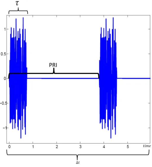
Figure 2.2: Radar Width and Pulse Repetition Interval
whereTris the round trip time of the radar pulse. Alternatively, the maximum unambiguous
range is [28]
Unambiguous Range :Ru =
cPRI
2 (2.9)
where the PRI calculated as the time between RADAR pulses. Figure 2.2 shows two radar pulses in an observation interval ∆t. The range resolution and accuracy is determined by the pulse’s durationτ, the speed of lightc, and the received signal to noise ratio (SNR) as in Equation (2.10) and Equation (2.11) respectively [28].
Range Resolution :∆R≈ cτ
2 (2.10)
Range Accuracy :δR ≈
cτ
2√2 SNR (2.11)
Range resolution represents the distance required between two distinct targets for the RADAR system to reliably distinguish between them. Equation (2.9), Equation (2.10), and Equation (2.11) provide information for characterizing the performance of a RADAR system. Performance improvements in RADAR systems have been towards greater spatial resolution capabilities of targets with noisy backgrounds [28].
The duty cycle of a constant amplitude pulsed signal is the ratio of the average transmit power over the PRI and the peak transmit power within a pulse [28].
δc = τ PRI = Pavg P0 (2.12)
The average transmit power Pavg is the instantaneous transmitted pulse power’s integral
over the PRI divided by the PRI and the peak transmitted power P0 is calculated as the
transmitted pulse power’s maximum value over the pulse intervalτ.
Pavg = 1 PRI Z PRI 0 p(t)dt (2.13a) P0=max p(t)|τ0 (2.13b)
with the instantaneous power of the transmitted pulsep(t)=|s(t)|2.
Range rate, or Doppler, is how the RADAR determines target velocity relative to the RADAR system. The RADAR to target range rate, resolution, and accuracy are given by [28]
Range-Rate :Rdot =
fdλ
2 (2.14a)
Range-Rate Resolution : ∆Rdot=
λ
2τ (2.14b)
Range-Rate Accuracy :δRdot =
λ
There is a trade-offbetween range and range-rate resolution and accuracy determined by the pulse length τ. A long pulse width is desired for acute Doppler resolution and accuracy while a short pulse is desired for fine range resolution and accuracy. However, pulsed radar can achieve both good range and range-rate resolutions through the use of pulse compression techniques. The pulse compression modulations considered in this research are LFM chirped, Barker coded, Frank coded, and Pxcoded waveforms.
Pulse compression waveforms allow the receiver to separate targets with overlapping received pulse returns. A compression filter is used to produce a narrow or compressed pulse from the pulse compression modulated received signal. The duration of the pulse is therefore reduced in the receiver and results in a better range resolution than was expected from the transmitted pulse duration [28]. Therefore, pulse compression modulation grants the increased Doppler range resolution of a long-pulse while retaining the range resolution of a narrow-pulse through received echo processing [8].
LFM was the first and still is a widely used pulse compression method. In LFM, the frequency of the signal is swept linearly during the pulse’s durationτover a bandwidthW
at the rate Wτ. The effective time-bandwidth product of LFM isW×τand contributes to the increased range resolution of a LFM pulse over a simple sinusoidal pulse. The equation for LFM is [21] LFM :s(t)=Rect t τ cos 2πt f0+ W 2τt , 0≤t ≤τ (2.15)
whereW is the bandwidth that is linearly swept during the pulse durationτand f0 is the
center frequency. Using a pulse compression receiver, the range resolution is [21]
∆R≈ c
2W (2.16)
which is dependent on the LFM’s bandwidth instead of its pulse duration as in Equation (2.10).
The next few pulse compression methods use phase-coded RADAR. Instead of linearly sweeping frequency in a pulse durationτ, phase-coding divides the pulse into M
Table 2.1: Known Barker codes [21] Code Length Code
2 11 or 10 3 110 4 1110 or 1101 5 11101 7 1110010 11 11100010010 13 1111100110101
sub-pulses which are assigned a phase value according to a specific phase code sequence. To maintain consistent notation with the communication waveforms, the sub-pulse duration will be referred to asTsymand is calculated asTsym= Mτ [21].
The next pulse compression method uses a very popular and common family of codes known as Barker codes. Barker codes ofMlength yield a max peak-to-peak sidelobe ratio of M. There are only nine known Barker codes [21], all listed in Table 2.1; however, Barker codes can be nested to produce larger, sub-optimal sequences such as the length 20 Barker4,5nested code as shown in Figure 2.3. Bi-phase Barker coded RADAR waveforms
are expressed as [21]
Bi-phase Barker : sm(t)= Rect t
τ
cos (2πfct+cmπ) , mTsym≤t ≤(m+1)Tsym (2.17)
wherecmis themthvalue of a known Barker code listed in Table 2.1.
Frank and Px codes apply for phase sequences of perfect square length M= L2where
smfor (1≤ m≤ M) is equal to s(l1−1)L+l2 for 1 ≤l1 ≤ Land 1 ≤ l2≤ L. These phase codes
produce improved range-rate resolution and accuracy over Barker phase codes [21]. Their sequences are calculated from [21]
s(l1−1)L+l2(t)=cos 2πfct+φl1,l2
Barker 4,5Nested Code Barker4 = 1101 Barker 5= 11101 1 1 1 0 1 1101 1101 1101 1101 1101 1 1 0 1 1 1 0 1 1 1 0 1 0 0 1 0 1 1 0 1 NOT Barker 4,5 =
Figure 2.3: Example of nested Barker4,5 code
Table 2.2: Some Frank Code Phase Sequences [21] Code Length Code
1 0
4 0, 0, 0, π
9 0, 0, 0, 0, 23π, 43π, 0, 43π, 83π
Table 2.3: Some PxCode Phase Sequences [21]
Code Length Code
1 0 4 π4, −4π, −4π, π4 9 π3, −3π, −π, 0, 0, 0, −3π, π3, π where Frank :φl1,l2 =2π(l1−1) (l2−1)/L (2.19a) Px :φl1,l2 = 2π L h(L+1) 2 −l2 i h(L+1) 2 −l1 i , Leven 2π L hL 2 −l2 i h(L+1) 2 −l1 i , Lodd (2.19b)
Frank phase codes produce linearly stepped linear phase segments as do Px codes
except Px codes have their zero phase-rate segment terms in the middle of the pulse instead
of at the beginning [21]. Phase values for the first three square Frank and Px phase codes
2.2 Pattern Recognition
Pattern Recognition has become a very useful tool with applications in many areas including electronic warfare (EW) and Cognitive software defined radio (SDR). Pattern recognition research for selecting and extracting features, developing classifier learning algorithms, and evaluating classifier performance is still prevalent in the literature [1, 5, 7, 19]. For most applications, there are two main methods of pattern recognition that are being used for modulation classification: likelihood-based and feature-based. The likelihood-based approaches strive to minimize false classification and theoretically can achieve near optimal performance, but are impractical in application due to computational complexity. Feature-based methods are much more computationally efficient and have been shown to achieve near optimal performance in the Bayesian sense [5]. A survey of current literature addressing both methods as applied to communication modulation classification was presented in [5] and an example of feature-based classification for radar waveform classification has been presented in [23].
2.2.1 Likelihood-Based Tests.
Likelihood based classification methods hinge on accurately modeling the signal of interest and all other ‘non-signal’ components that comprise the received signal ’s probability distribution. Decisions are made by comparing likelihood ratios against a threshold. Among likelihood-based approaches, two ways to model the received signal’s probability distribution are the average likelihood ratio test (ALRT) and generalized likelihood ratio test (GLRT) [5]. Depending on the information knowna prioriabout the signals being discriminated, either the ALRT or the GLRT is used.
The ALRT method treats received unknown variables as random variables with assumed known probability density functions (PDFs), but the GLRT method treats the received unknown variables as deterministic unknowns. Therefore the GLRT method does not make any assumptions about the signal or the channel parameters. The final decision is
then based on a maximun likelihood (ML) comparison [5, 22]. For a binary classification problem, Lj[H1|r(t)] Lj[H0|r(t)] H1 ≷ H0 λj , j= A(ALRT), G(GLRT) (2.20)
whereλj is a threshold and the method used to compute the likelihood functions Lforms
either the ALRT or GLRT on the left side. H1 represents decision ‘1’, H0 represents
decision ‘0’ in this binary case, andr(t) is the received waveform
2.2.2 Feature Based Tests.
Feature-based classification methods use extracted statistics, or features, from a received signal to make classification decisions based on the reduced data set. This reduced data set is called a feature vector and is represented by ψ. Some examples of discriminating features include symbol rates, signal magnitude variance, duty cycle, instantaneous frequency, instantaneous phase, cumulants, and many others. Many feature-based methods require somea prioriknowledge of signal parameters in order to accurately calculate signal features. The extracted signal features are then used for decision making. Decision making methods are usually based on feature PDFs, or feature vector distances from calculated class feature vector means [5].
In literature, cyclostationary-based features have gained popularity as potential features for modulation recognition because they are insensitive to unknown signal and channel parameters and preserve signal phase information [22]. In [27], the received signal’s fourth-order two conjugate cumulants were used as features to discriminate between BPSK, 4-ASK, 16-QAM and 8-PSK when carrier phases, frequency offsets, and timing offsets were unknown.
2.3 Cyclostationarity
A stationary random process is one where all its joint moments are non-varying and all its functions’ expected values are stationary. wide-sense stationary (WSS) is a weaker
form of stationarity, which requires only the 1st and 2nd order statistics to be stationary (not vary with a shift in the time origin). Therefore, a WSS random process has a mean (µx) and autocorrelation (Rx) that satisfy the following conditions [11, 20]:
E[x(t)]=µx , ∀t Rx(t, τ)=Rx(τ) 4 =E x t+ τ 2 x∗ t− τ 2 , ∀t
whereτis some time delay. Both statistics are independent of the time origin (t) and the auto-correlation function only depends on the time difference (τ) between samples. All stationary random processes are WSS, but not all WSS processes are stationary [20].
Instead of non-varying means and autocorrelations, wide-sense cyclo-stationary (WSCS) random processes have periodic means and autocorrelations [15]. Therefore, for cyclostationary random processes, the mean (µx) and autocorrelation (Rx) are periodic for
some periodT0 and satisfy the following conditions [11]: E[x(t+T0)]=µx(t+T0)=µx(t), ∀t Rx(t+T0, τ)=Rx(t, τ) 4 = E x t+ τ 2 x∗ t− τ 2 , ∀t
RF waveforms commonly exhibit cyclostationary properties due to common operations such as modulating, coding, multiplexing, and sampling which induce periodicities in the statistics of the signals. The periodicities in autocorrelation produce spectral correlations which can be exploited for signal processing [10].
To accurately calculate µx(t) and Rx(t, τ), we would have to use ensemble averaging
over many observations of a single process and have knowledge of PDFs. However, if time averaging over a single observation is equal to ensemble averaging over many observations, the random process can be described as ergodic. It is a reasonable assumption for most waveforms used in communication and radar applications that the first and second-order statistics within the transmitted waveform satisfy the ergodic property [26]. Therefore, to avoid an unnecessary probabilistic discussion, signals in this paper are assumed to be ergodic in the mean and autocorrelation function. This allows us to treat the temporal
average as equivalent to the expected value, or ensemble average [20]. In this thesis, temporal averaging with respect totwill be denoted ash·it.
E[·]=h·it =4 lim T→∞ 1 T Z T/2 −T/2 (·)dt≈ lim N→∞ 1 2N+1 N X n=−N (·) (2.21) 2.3.1 Theory.
In order to derive the mathematical representation of cyclostationarity and, in turn, produce the SCF, it is easiest to start from simple frequency analysis. Time limited and periodic signals can be expanded into a summation of weighted sinusoids known as a Fourier Series x(t)=4 +∞ X n=−∞ Xne j2π T0nt =4 +∞ X n=−∞ Xnej2πn f0t, n∈I (2.22)
where f0, the inverse of the period, T0, is the fundamental frequency, I denotes an
integer set, and the coefficients Xn are the sinusoidal component weights at frequencies
f = Tn
0 = n f0. Therefore, if a signal has a non-zero Fourier Series, it has the additive sinusoidal components of frequency f with weights Xngiven by
Xn 4 = lim T→∞ 1 T Z T/2 −T/2 x(t)e−j2πn f0tdt. (2.23) Let us assume that the signal x(t) contains a finite frequency component given by
a cos (2παt), where a is the frequency magnitude component at f = α. Therefore, the
complex Fourier Series coefficient ofx(t) at frequencyαmay be represented by [10, 11, 15]
Mαx = lim T→∞ 1 T Z T/2 −T/2 x(t)e−j2παtdt (2.24a) =D x(t)e−j2παtE t. (2.24b)
2.3.2 Cyclic Autocorrelation Function.
Now let’s progress to a signal produced by the lag-product of another signal. This quadratic transformation produces
y(t, τ)= x t+ τ 2 x∗ t− τ 2 (2.25) where (·)∗ denotes the complex conjugate andτ is a time delay. The signaly(t) contains additive sinusoidal components if and only if
Myα(τ)= D y(t, τ)e−j2παtE t = x t+ τ 2 x∗ t− τ 2 e−j2παt t , (2.26)
is non-zero for any frequencyα,0.
It may be apparent that Equation (2.26), the Fourier Coefficients of the lag-product
Myα(τ), is a generalized formula of the conventional autocorrelation function ofx,Rx(τ). It
can be shown that in the special case whereα= 0,Mαy=0(τ) is equivalent to the conventional
autocorrelation functionRx(τ). Myα=0(τ)= D y(t, τ)e−j2π0tE t = hy(t, τ)it = x t+ τ 2 x∗ t− τ 2 t (2.27a) Rx(τ)= E x t+ τ 2 x∗ t− τ 2 = x t+ τ 2 x∗ t− τ 2 t (2.27b) Therefore, Myα=0(τ) = Rx(τ) = D xt+ τ2x∗t− τ2E t and M α y(τ) may be interpreted as
an autocorrelation function of x(t) with a cyclic weighting factor of e−j2παt. In literature,
Myα(τ) is commonly expressed as the cyclic autocorrelation function (CAF) and is written
as [10, 11, 13, 15] Rαx(τ)=4 lim T→∞ 1 T Z T/2 −T/2 Rx(τ)e−j2παtdt (2.28a) =D Rx(τ)e −j2παtE t (2.28b) =x t+ τ 2 x∗ t− τ 2 e−j2παt t . (2.28c)
By definition, Equation (2.28) is not identically zero as a function of τif and only if x(t) contains second-order periodicity with frequencyα,0. Therefore, the CAF highlights the
second-order periodicities with frequencyα in the signal x(t). Also, Equation (2.28) has the same form as Equation (2.24) which tells us that Rαx(τ) is a Fourier coefficient in the
Fourier series expansion ofRx(τ) [10].
Rx(τ) 4 = ∞ X n=−∞ Rαx(τ)ej2παt , α= n T , n∈I (2.29)
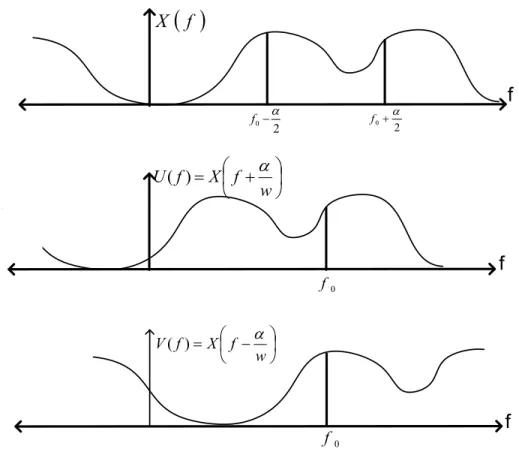
Instead of an autocorrelation function with a cyclic weighting factor, the CAF can also be interpreted as a conventional cross-correlation between two identical signals separated byαin frequency. Letu(t) andv(t) be the signal x(t) multiplied bye±j2πα2t which shifts the frequency components ofx(t) by∓α2 as illustrated in Figure 2.4.
u(t)=x(t)e−j2πα2t (2.30a)
v(t)=x(t)ej2πα2t (2.30b)
The Fourier transforms ofu(t) andv(t) show that their frequency spectrums are
U(f)= F [u(t)]= F hx(t)e−j2πα2ti= X f + α 2 (2.31a) V(f)= F [v(t)]= F hx(t)e+j2πα2ti= X f − α 2 (2.31b)
and the Wiener-Khinchin relation tells us that the Fourier transforms of Ru(τ) and Rv(τ)
give us their Power Spectral Densities (PSDs) [3, 12, 20].
Su(f)=Sx f + α 2 (2.32a) Sv(f)=Sx f − α 2 . (2.32b)
Defining u(t) and v(t) as frequency shifted versions of x(t) leads us to an important conceptual understanding of the CAF. It can be shown that the conventional
cross-2 0 a + f 0 f 0 f 2 0 a -f ÷ ø ö ç è æ + = w f X f U( ) a ÷ ø ö ç è æ -= w f X f V( ) a
( )
f Xf
f
f
Figure 2.4: Frequency spectrum of frequency translatesu(t) andv(t) of x(t)
correlation ofu(t) andv(t) equals the CAF of x(t).
Ruv(τ) 4 =E u t+ τ 2 v∗ t− τ 2 (2.33a) =u t+ τ 2 v∗ t− τ 2 t (2.33b) =x t+ τ 2 e−jπα(t+τ/2) × x t− τ 2 ejπα(t−τ/2) ∗ t (2.33c) =x t+ τ 2 x∗ t− τ 2 e−j2παt t = Rαx(τ) (2.33d) Ruv(τ)=Rαx(τ)
This illustrates the interpretation that the CAF is simply a temporal cross-correlation between frequency-shifted versions of a signal.
2.3.3 Spectral Correlation Function.
According to the Wiener-Khinchin and cyclic Wiener-Khinchin relations, the Fourier transform of the autocorrelation function is the power spectral density (PSD) and the Fourier transform of the CAF is the SCF [12, 13].
Sx(f)= Z ∞ −∞ Rx(τ)e−j2πfτdτ= F [Rx(τ)] (2.34a) Sαx(f)= Z ∞ −∞ Rαx(τ)e−j2πfτdτ=F Rαx(τ) (2.34b) The SCF is represented on a bi-frequency plane because it is a function of both frequency,
f, and cyclic frequency, α. Just as the conventional autocorrelation function is a special case of the CAF for whenα= 0, the PSD is included in the SCF as the special case when α = 0. Remember from Equation (2.33) that the cross-correlation ofu(t) and v(t) equals the CAF ofx(t). It follows that
Sαx(f)= F
Rαx(τ)
= F
[Ruv(τ)]= Suv(f) (2.35)
where Suv(f) is the spectral density of cross correlation between u(t) and v(t) at
the frequency f and Sαx(f) is the spectral density of correlation between the spectral
components of x(t) at f − α2 and f + α2. The SCF of x(t) is the Fourier transform of the temporal cross-correlation between frequency-shifted versions ofx(t).
Suppose that x(t) in u(t) and v(t) in Equation (2.30) are band-limited with a double-sided bandwidth 2B. The SCF region of support for a band-limited signal is illustrated in Figure 2.5. At the cyclic frequency of α = 0, all spectral components of the correlated frequency translates of x(t) overlap. However, for the cyclic frequency α = −B, only spectral components from −B2 to B2 overlap and therefore Sα=−B
x (f) only supports the
frequency region −B2 ≤ f ≤ B2. The frequency translates have no overlapping spectral
components when|α|> 2B.
In [13] and [14], the SCF for analog and digital modulated signals are derived. It is shown that signals with the same power spectral densities may have distinct cyclic
f
f f f)
(
f
X
) (f 2B X ) (f B X ) (f B X 2 B 2 B B B )
(
f
S
x B ) (f 2B X ) ( 2 f Sx B)
(
0f
S
xB
B
B 2 B 2 B B Figure 2.5: SCF Support Region for the Band-limited Signalx(t).
spectrums. Also, the cyclic spectrum is shown to be robust to additive white gaussian noise (AWGN) because stationary noise has no cyclic correlation. Therefore, distinguishing signal features may be extracted from the SCF and can be used for robust classification in varying noise environments. Techniques for estimating the SCF from sampled data are explored in Section 2.4.
2.4 Estimating the Spectral Correlation Function
The theoretical SCF equations presented thus far deal with signals of infinite time duration. In practice, only finite time observations of a signal are available for analysis and, as such, a substantial amount of work has been done to modify the underlying equations to produce efficient, accurate SCF estimates. In general, temporal and frequency smoothing are the two methods used to produce these estimates. Both methods derive from the SCF
cyclic periodogram estimate [9, 10, 25]. SαxT(t, f)= XT t, f + α 2 X∗T t, f − α 2 (2.36) where XT(t, f)= Z ∞ −∞ aT(t−u)x(u)e−j2πf udu (2.37a) =Z t+T/2 t−T/2 x(u)e−j2πf udu (2.37b)
is the finite time Fourier transform ofx(t) withaT(t−u), a data tapering window of width
T. In the context of Spectral Correlation,XT(t, f) is commonly referred to in literature as a
complex demodulate. For statistical reliability, and a reliable estimate, the time-bandwidth product should be much greater than 1 (∆t×∆f 1) [25]. The cyclic periodogram in Equation (2.36) has a temporal resolution dictated by the data tapering window aT(t−u)
in XT(t, f) giving ∆t = T. The frequency resolution is also dictated by the data tapering
window size, ∆f ≈ T1 ≈ ∆1t. The resulting time-bandwidth product of Equation (2.36) is
∆t∆f ≈∆t∆1t ≈1.
Applying time-smoothing to Equation (2.36) gives the time-smoothed cyclic peri-odogram SαxT(t, f)∆t = ∞ Z −∞ SαxT(u, f)·h∆t(t−u)du (2.38a) = ∞ Z −∞ XT u, f + α 2 X∗T u, f − α 2 h∆t(t−u)du (2.38b)
where the new time resolution is defined by ∆t, the width of the sliding data tapering window function h∆t(t − u). To maintain statistical reliability, the data tapering window
function should have a width∆t ∆1f ≈ T so that the time bandwidth product∆t×∆f 1. Applying frequency-smoothing to Equation (2.36) gives the frequency-smoothed cyclic
periodogram Sαx T(t, f)∆f = ∞ Z −∞ Sαx T(t,v)·h∆f(f −v)dv (2.39a) = ∞ Z −∞ XT t,v+ α 2 XT∗ t,v− α 2 h∆f(f −v)dv (2.39b)
where the new frequency resolution is defined by ∆f, the bandwidth of the bandpass filterh∆f(f −v). To maintain statistical reliability, the bandwidth of h∆f(f −v) should be ∆f ∆1
t = 1
T so that the time bandwidth product ∆t×∆f 1. It can be shown that both
the time-smoothed cyclic periodogram and the frequency-smoothed cyclic periodogram approach perfect estimations of the SCF when the following limits are applied [10, 13]
Sαx(f)= lim T→∞∆limt→∞S α XT (t, f,)∆t (2.40a) = lim ∆f→0Tlim→∞S α XT (t, f,)∆f (2.40b)
Both estimates produce a cyclic frequency resolution ∆α ≈ 1
∆t and it follows that to
maintain reliable estimates∆f ∆1
t ∆α. Therefore, the SCF estimate must have finer
resolution in cyclic frequency (α) than in spectral frequency (f) to be statistically reliable. The time smoothing and frequency smoothing methods are generally well suited for different applications of SCF estimation. In general, variants of the time-smoothed cyclic periodogram are well suited for efficient estimation over the entire bi-frequency plane, whereas, variants derived from the frequency-smoothed cyclic periodogram are more suited for estimating the SCF at particular cyclic frequencies [22, 25].
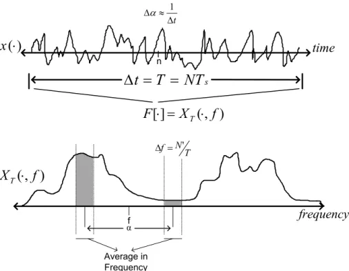
2.4.1 Temporal Smoothing.
All temporal smoothing algorithms for estimating the SCF are derived from the temporally smoothed cyclic periodogram given in Equation (2.38). Incorporating the data
tapering function into the integral and simplifying reduces the equation to Sαx T(t, f)∆t = ∞ Z −∞ Sαx T(t, f)·h∆t(t−u)du = t+∆t Z t SαxT(t, f)du= 1 T t+∆t Z t XT u, f + α 2 X∗T u, f − α 2 du =1 T XT t, f + α 2 X∗T t, f − α 2 ∆t (2.41) where the complex demodulate,XT(t, f), is defined as in Equation (2.37). In [25] and [22],
Equation (2.38) was extended to discrete, sampled time-series.
Sα0X T n, f0∆t = n+N X r=n XTr, fkXT∗ r, flh∆t[n−r] (2.42) whereα0 = fk − fl , f0 = fk+fl
2 , ris a dummy variable, andXT
r, fkis the discrete version
of Equation (2.37) given by XTr, fk= N0−1 X m=0 aT[m]x[r+m]e−j2πfk(r+m)Ts (2.43a) = N0−1 X m=0 aT[m]x[r+m]e−j2πk(r+m)/N 0 (2.43b) where x[n] = x(t)|t=nTs, Ts = 1 2B, fk = k N0T s, and T = N 0T
s. The temporal resolution ∆t = NTs and the frequency resolution ∆f = N10T
s which produces a time bandwidth
product∆t∆f = NN0 and cyclic frequency resolution∆α≈ 1
∆t = 1
NTs. For statistical reliability N N0 and∆α ∆f [25].
Equation (2.41), Equation (2.42), and Figure 2.6 show that the time smoothed cyclic cross periodogram is basically a correlation between the spectral components ofx[n] over the time observation of∆t. The time smoothing is done by allowing a data tapering window of length T time to slide over the total signal observation ∆t time or equivalently a data tapering window of length N0 samples to slides over the total data samples of length N.
Again, the window of size N0 samples or T time should be much smaller than the total observation length ofNsamples or∆ttime for statistically accurate estimates [22, 25].
time
sNT
t
=
D
n s T N T= ')
(
×
x
)
,
(
]
[
X
f
F
×
=
T×
time
frequency Average in Time a D = Dt 1 f α Df =1T)
,
(
f
X
T×
Figure 2.6: Temporal Smoothing [25]
Since this method is deemed computationally inefficient, ways to improve the computational efficiency of the time-smoothed spectral estimates were explored in [25]. One method to improve the computational efficiency is to decimate Equation (2.43) by L, where L < N0, giving XTrL, fk. This reduces the number of correlations in
Equation (2.42) by a factor of L from N to P = NL. Equivalently, instead of calculating Equation (2.43)Ntimes, then decimating toPvalues, a system can simply calculate theP
values ofXTrL, fkby shifting x[n] byLsamples each computation. A decimation factor
of L = N40 has been shown to be a good choice to increase computational efficiency and minimize adverse effects from cycle leakage and cycle aliasing [4]. The time smoothing with decimation cyclic periodogram is [25]
Sα0X T nL, f0∆t = n+P X r=n XTrL, fkXT∗ rL, flh∆t[n−r] (2.44)
where XTrL, fk= N0−1 X m=0 aT[m]x[rL+m]e−j2πk(rL+m)/N 0 (2.45) Another method to improve the cyclic spectral estimates computational efficiency is to multiply both sides of Equation (2.42) with the sinusoidal factor e−j2πqm/N. This shifts
the left side in cyclic frequency by Nq = q∆αwhereq = [0,1,· · · ,N−1] and fits the right side into the form of anN-point fast fourier transform (FFT) [25].
SαX T n, f0∆t e−j2πqm/N = N X r=0 XTr, fkXT∗ r, flh∆t[n−r] e−j2πqr/N (2.46a) Sα1X+q∆α T n, f0∆t =F XTr, flX∗T r, fk?h∆t[r]N (2.46b) =F XTr, flX ∗ T r, fkNF [h∆t[r]]N (2.46c)
where ?denotes a convolution, the notation F [·]N denotes an N-point DFT, XTr, fk is
computed as in Equation (2.43), f0 = fk+fl 2 = k+l 2 f s N0 , and α0 = fk − fl = (l−k) f s N0 . Utilizing the concepts above, [25] presents the FFT accumulation method (FAM) and strip spectral correlation algorithm (SSCA) as computationally efficient time smoothing algorithms to estimate the cyclic spectrum.
2.4.1.1 FFT Accumulation Method.
The FAM applies both decimation and FFTs to Equation (2.42), resulting in
Sαi+q∆α XT nL, f0∆t = P−1 X r=0 XTrL, fkXT∗ rL, flh∆t[n−r]e−j2πqr/P (2.47a) = N L−1 X r=0 XTrL, fkXT∗ rL, flh∆t[n−r]e−j2πqrL/N (2.47b) =F XTrL, fkX∗T rL, flPF [h∆t[r]]P (2.47c)
where XTrL, fk is defined as in Equation (2.45), α0 = αi + q∆α, L is the decimation
factor, andP= NL. The time and frequency resolutions are∆α= fs PL = fs N,∆t= 1 ∆α = Nfs, and ∆f q = ∆ a− |q|∆α. Since∆a = fs N0, ∆f q can be reduced to1− |q|PLN0 fs N0. Therefore,
f D
a
Df
a
2 s f 2 s f -s f -s fFigure 2.7: FAM Estimate Resolution [22, 25]
Figure 2.7 shows the support region for the FAM. To minimize the point estimates near the top and bottom of the channel-pair regions, whereq is large and the time bandwidth product is reduced resulting in less reliable estimates, only the estimates within the region center±∆a/2 are retained. This leaves only the terms corresponding to
−∆a 2 ≤q∆α ≤ ∆a 2 − N 2N0 ≤ q ≤ N 2N0 −1 − PL 2N0 ≤ q ≤ PL 2N0 −1
Therefore, there are missing estimates for some cyclic frequencies,α, where the estimates are less reliable. These missing estimates may contain important cyclic features and therefore, the FAM is not advised when location of cyclic features is unknowna priori.
f D
a
Df
a
0 0=2fk-2f a a D + =f q k 2 s f 2 s f -s f -s fFigure 2.8: SSCA Estimate Resolution [22, 25]
2.4.1.2 Strip Spectral Correlation Algorithm.
The second temporally-smoothed cyclic spectral estimation algorithm is the SSCA, which allows estimates of all cyclic frequencies. In this algorithm, the complex demodulates XTn, fk directly multiply with x∗(n), which produces estimates along the
frequency-skewed lineα= 2fk−2f0. This algorithm has been shown to give highly efficient
estimates of the SCF over the entire bi-frequency plane, but sacrifices fine frequency resolution [25]. The SSCA is given by
Sfk+q∆α XT " n, fk 2 −q ∆α 2 # ∆t = N X r=0 XTr, fkx∗[r]h∆t[n−r]e−j2πqr/N (2.48a) =F XTr, fkx∗[r]NF [h∆t[r]]N (2.48b) whereα0 = fk+q∆αand f0 = fk 2− q∆α
2 . The temporal and frequency resolutions are∆t = N fs, ∆f = T1 = fs N0, and∆α≈ 1 ∆t = fs
N making the time-bandwidth product∆t∆f = N
N0. Like the
2.4.2 Frequency Smoothing.
The frequency-smoothed cyclic periodogram equation was given in Equation (2.39). In [4] and [22], Equation (2.39) was extended to discrete sampled time-series.
Sα0X T n, f0∆f = N0 2−1 X r=−N20 XT n, fk + r T XT∗ n, fl+ r T h∆f[r] (2.49) whereα0 = fk− fl, f0 = fk+fl
2 ,h∆f[r] represents the response of some bandpass filter with
bandwidth∆f, and the complex demodulate
XTn, fk= N−1 X
m=0
aT[m]x[n+m]e−j2πfk(n+m)Ts (2.50)
is now calculated from N samples instead of N0 samples. Figure 2.9 gives a graphical representation of Equation (2.49). The temporal and frequency resolutions for the frequency-smoothed SCF are∆f = NT0 = NTN0
s, ∆t = T = NTs, and∆α ≈ 1
∆t. The
time-bandwidth product is then, ∆t∆f = N0 and we let N0 1 for statistical reliability. It is apparent from Equation (2.49) that there is a trade-off between statistical reliability and spectral resolution [25]. To achieve highly reliable SCF estimates, a large amount of frequency smoothing is desired, but if the spectrum has narrow spectral features, the amount of spectral smoothing should be minimized [25].
2.5 Cyclic Cumulants
Statistics are used to describe and characterize the behavior of processes. Specifically, the moments and cumulants of processes are very useful for describing behavior. Since cumulant functions generally can not be computed from experimental time-series data, they are usually estimated from knowledge of moment functions, which can be computed from experimental data [3]. Temporal and spectral cumulants are shown theoretically to exhibit the property of signal selectivity in [16]. This is the ability to to detect or estimate parameters of a specific signal in a received waveform even when corrupted by noise or
time s
NT
T
t
=
=
D
n)
(
×
x
)
,
(
]
[
X
f
F
×
=
T×
frequency Average in Frequency t D » Da 1 α T N f = ' D)
,
(
f
X
T×
fFigure 2.9: Frequency Smoothing
interference. This property was verified through simulations in [27]. The temporal moment function (TMF) for zero time-lag is [3]
Rx(t, τ=0)n,q 4 = E
x(t)n−q (x∗(t))q
(2.51) and is used to computen-order,q-conjugate moments. It is apparent that the autocorrelation defined in Equation (2.27b) is a specific case of the TMF with n = 2 and q = 1 so
Rx(t, τ)2,1 = E[x(t)x ∗
(t)]. Using the moments, cumulants are calculated through the moment to cumulant formula, also known as the temporal cumulant function (TCF) [16, 17]
Cx(t, τ)n,q = X Pn (−1)p−1(p−1)! p Y j=1 Rx(t, τ)nj,qj (2.52)
where Pn are all distinct partitions of the set [1,2,· · · ,n], pis the number of elements in
each partition, andRx(t, τ)nj,qj is then-order,q-conjugate moment corresponding to the jth
Table 2.4: n=4, q=2 cumulant partitions where (·)∗ denotes a conjugate and ‘1’ and ‘2’ were generically chosen as the two conjugated terms.
n=4,q=2 Partitions Cx(t)4,2 Partitions p Pn (−1)p−1(p−1)! p Q j=1 Rx(t,0)nj,qj 1 (1∗,2∗,3,4) Rx(t)4,2 2 (1∗,2∗) (3,4) − Rx(t)2,2Rx(t)2,0 2 (1∗,3) (2∗,4) − Rx(t)22,1 2 (1∗,4) (2∗,3) −Rx(t)22,1 2 (1∗,2∗,3) (4) −R x(t)3,2Rx(t)1,0 2 (1∗,2∗,4) (3) −Rx(t)3,2Rx(t)1,0 2 (1∗,3,4) (2∗) −Rx(t)3,1Rx(t)1,1 2 (2∗,3,4) (1∗) −R x(t)3,1Rx(t)1,1 3 (1∗,2∗) (3) (4) 2R x(t)2,2Rx(t)21,0 3 (1∗,3) (2∗) (4) 2Rx(t)2,1Rx(t)1,1Rx(t)1,0 3 (1∗,4) (2∗) (3) 2Rx(t)2,1Rx(t)1,1Rx(t)1,0 3 (2∗,3) (1∗) (4) 2R x(t)2,1Rx(t)1,1Rx(t)1,0 3 (2∗,4) (1∗) (3) 2Rx(t)2,1Rx(t)1,1Rx(t)1,0 3 (3,4) (1∗) (2∗) 2Rx(t)2,0Rx(t)21,1 4 (1∗) (2∗) (3) (4) −6R x(t)21,1Rx(t)21,0
values for zero delay values, τ = 0 [6]. Therefore, all n-order moments and cumulants in this research are calculated for τ = 0 and τ will be omitted from the notation. For example,Cx(t, τ)4,2will be expressed asCx(t)4,2. In Table 2.4 an example for calculating
the terms forCx(t)4,2 from Equation (2.52) is shown. There are 15 distinct partitions of the
set [1∗,2∗,3,4] where there are n = 4 items andq = 2 are conjugated. Item ‘1’ and item ‘2’ in the set were generically chosen as the two conjugated terms, but any combination of two may be chosen as long as the selections are maintained throughout the derivation. Summing theCx(t)4,2 partition terms in Table 2.4 gives Equation (2.53).
Cx(t)4,2 =Rx(t)4,2− Rx(t)2,0 2 −2Rx(t)22,1−2Rx(t)3,2Rx(t)1,0−2Rx(t)3,1Rx(t)1,1 +2Rx(t)2,2Rx(t)21,0+8Rx(t)2,1 Rx(t)1,0 2 +Rx(t)2,0Rx(t)21,1−6 Rx(t)1,0 4 (2.53)
Table 2.5: Cumulants Cn,q Equation C2,0 R2,0 C2,1 R2,1 C4,0 R4,0−3C22,0 C4,1 R4,1−3C2,0C2,1 C4,2 R4,2− C2,0 2 −2C22,1 C6,0 R6,0−15C2,0C4,0−15C32,0 C6,1 R6,1−10C2,0C4,1−5C2,1C4,0−15C2,1C22,0 C6,2 R6,2−C2∗,0C4,0−8C2,1C4,1−6C2,0C4,2−3C2∗,0C 2 2,0−12C2,0C2c,1 C6,3 R6,3−3C2∗,0C4,1−9C2,1C4,2−3C2,0C∗4,1−9C∗2,0C2,1C2,0−6C23,1 C8,0 R8,0−28C2,0C6,0−35C24,0−210C 2 2,0−105C 4 2,0
The cumulant equation is greatly simplified when central moments are used instead of raw moments, or the process is known to be a zero mean process, µx = Rx(t,0)1,0 = Rx(t,0)1,1 = 0. In practical situations, a signal can be made a zero mean process by
subtracting the mean from it.Cx(t,0)4,2reduces to Cx(t)4,2 =Rx(t)4,2− Rx(t)2,0 2 −2Rx(t)22,1. (2.54)
A list of the zero-mean cumulant equations derived from Equation (2.52) as functions of lower order moments and cumulants are shown in Table 2.5. Owing to the symmetrical signal constellations considered, thenth-order moments for n odd are zero and therefore, thenth-order cumulants fornodd are also zero and have been dropped from the cumulant equations in Table 2.5 [5].
Much like the CAF is found by Fourier transforming the autocorrelation function, the cyclic temporal cumulant function (CTCF) is produced by Fourier transforming the TCF [16] Cβx(t,0)n,q = ∞ Z −∞ Cx(t,0)n,qe−j2πβtdt (2.55)
which gives the TCF’s frequency components at frequency β. Thenth-order,q-conjugate cycle frequencies (CFs) of interest are atβ = (n−2q) fc [6]. Since AWGN is a stationary,
zero-mean Gaussian process, its cumulants are time independent and non-zero only for the second order. Therefore, AWGN does not have any contribution to the higher-order (n≥3) cyclic cumulants (CCs) of a received signal r(t). Last, the magnitude of the nth-order,
III. Methodology
T
hischapter outlines the work that led to the development of a modulation recognitionsystem. The modulation recognition system is feature-based and designed to discriminate between BPSK, QPSK, 16-QAM, 64-QAM, 8-PSK, 16-PSK, Barker5,
Barker11, Barker55, Frank49, Px49, and LFM modulations using features derived from
theory in Chapter II. All simulations were done in discrete-time with matrix laboratory (MATLAB®), therefore all equations will be presented for discrete-time.
Section 3.1 describes the process used to simulate the waveforms and Section 3.2 describes the process of introducing AWGN to the waveforms to simulate received SNR. Section 3.3 highlights how the features were estimated, Section 3.4 explains the classifier supervised training process, and Section 3.5 gives the metrics used to assess the classifier performance.
3.1 Simulating Modulations
This section describes the process used to simulate the waveforms being considered in this research. The process used to simulate the waveforms in MATLAB® is shown in Figure 3.1.
Equation (3.1) is the discrete version of Equation (2.4) and is used to simulate the discrete symbols for BPSK, QPSK, 8-PSK, and 16-PSK
BPSK : sm[n]=Acos (2πfcnTs+π(m−1)) m= 1,2 (3.1a) QPSK : sm[n]=Acos 2πfcnTs+ π 2(m−1) m= 1,2,3,4 (3.1b) 8-PSK : sm[n]=Acos 2πfcnTs+ π 4(m−1) m= 1,2,· · · ,8 (3.1c) 16-PSK : sm[n]=Acos 2πfcnTs+ π 8(m−1) m= 1,2,· · · ,16 (3.1d)
Pick Waveform Generate Random Communication Symbols Generate Radar Pulse
BPF
Raised Cosine PulseShaping Filter
Simulated Waveform
Figure 3.1: Waveform Simulation Process
where each symbol is defined on the discrete interval 0 ≤ nTs ≤ Tsym, Tsym is the symbol
period, and Ts is the discrete sampling period related to sampling frequency by fs = T1
s.
Equation (3.2) is the discrete form of Equation (2.6) and is used to generate the 16-QAM and 64-QAM symbols
M-QAM :sm[n]=Amφ1(nTs)+Bmφ2(nTs) (3.2)
0≤nTs ≤Tsym m= 1,2,· · · ,M
where φ1(t) = cos (2πfcnTs), φ2(t) = sin (2πfcnTs), Am and Bm are defined as Am =
(2am−1)−
√
M and Bm = (2bm−1)−
√
M with amand bm all combinations of integers
in the seth1,2,· · · , √Mi. For 16-QAM,AmandBmmay have values [−3,−1,1,3] and for
64-QAM,AmandBmmay have values [−7,−5,−3,−1,1,3,5,7].
Since the information symbols in communication waveforms can be modeled as random, each generated communication symbol is uniformly randomly selected. This process was simulated by using the MATLAB® command ‘randi’ which uniformly randomly selects a value from a given set. The resulting communication waveform, s[n], consists of a stream of random symbols sm[n]. This produces pseudo random streams of
each modulation where all symbols are equally likely to occur every symbol period. Also, the signal’s modulated and transmitted information bandwidth isW = 2B= T2
Equation (3.3) is used for simulating an up-chirp pulse with bandwidth,Bcentered at carrier frequency fcwith durationτ.
LFM : s[n]=Rect nT s τ cos 2πnTs fc+ W 2τnTs , 0≤nTs ≤τ (3.3)
Equation (3.4) is used to simulate Barker5, Barker11, and Barker5,11 codes. Barker5 and
Barker11 use the codes given in Table 2.1 corresponding to length 5 and 11 respectively,
but Barker5,11 uses the code generated by ‘nesting’ the length 5 code within a length 11
code sequence similar to the Barker4,5example in Figure 2.3.
Barker :sm[n]= Rect
nT
s
τ
cos (2πfcnTs+cmπ) , mTsym ≤nTs ≤(m+1)Tsym (3.4)
Equation (3.5) is the discrete equation for Frank and Px coded radar pulses with the phases defined as in Equation (2.19).
s(l1−1)L+l2[n]=cos 2πfcnTs+φl1,l2
(3.5)
The radar pulse compression modulations are considered deterministic not random. Their value during a symbol period is predetermined by the specific code sequence corresponding to the pulse compression format/type.
After the waveform symbols are generated, they are filtered using a raised cosine pulse shaping filter in MATLAB® with 50% excess bandwidth and a roll-offfactorβ= 0.4. This filter was used to simulate the pulse shaping filter in a transmitter and to band-limit the transmitted simulated waveform. The impulse response of a raised cosine filter is given by
h[n]= sinc nTs Tsym ! cos πβnT s Tsym 1−2βnTs Tsym 2 (3.6)
This raised cosine filter was generated in MATLAB®using the ‘firrcos’ command with the options: filter order = 10, cutofffrequency = 1.5× Bwhere B = fS ym = T1
S ym , and
−20 −15 −10 −5 0 5 10 15 −0.05 0 0.05 0.1 0.15 0.2 0.25 0.3 Delay τ
(a) Impulse Response of Pulse Shaping Filter Used
s<

![Figure 2.6: Temporal Smoothing [25]](https://thumb-us.123doks.com/thumbv2/123dok_us/797950.2600866/41.918.218.717.130.547/figure-temporal-smoothing.webp)
![Figure 2.7: FAM Estimate Resolution [22, 25]](https://thumb-us.123doks.com/thumbv2/123dok_us/797950.2600866/43.918.301.622.104.475/figure-fam-estimate-resolution.webp)
![Figure 2.8: SSCA Estimate Resolution [22, 25]](https://thumb-us.123doks.com/thumbv2/123dok_us/797950.2600866/44.918.298.622.109.474/figure-ssca-estimate-resolution.webp)