Scholarship@Western
Scholarship@Western
Electronic Thesis and Dissertation Repository8-18-2020 10:00 AM
Ranking comments: An Entropy-based Method with Word
Ranking comments: An Entropy-based Method with Word
Embedding Clustering
Embedding Clustering
Yuyang Zhang, The University of Western Ontario
Supervisor: Yu, Hao, The University of Western Ontario
A thesis submitted in partial fulfillment of the requirements for the Master of Science degree in Statistics and Actuarial Sciences
© Yuyang Zhang 2020
Follow this and additional works at: https://ir.lib.uwo.ca/etd
Part of the Applied Statistics Commons, and the Data Science Commons
Recommended Citation Recommended Citation
Zhang, Yuyang, "Ranking comments: An Entropy-based Method with Word Embedding Clustering" (2020). Electronic Thesis and Dissertation Repository. 7300.
https://ir.lib.uwo.ca/etd/7300
This Dissertation/Thesis is brought to you for free and open access by Scholarship@Western. It has been accepted for inclusion in Electronic Thesis and Dissertation Repository by an authorized administrator of
Automatically ranking comments by their relevance plays an important role in text mining and text summarization area. In this thesis, firstly, we introduce a new text digitalization method: the bag of word clusters model. Unlike the traditional bag of words model that treats each word as an independent item, we group semantic-related words as clusters using pre-trained word2vec word embeddings and represent each comment as a distribution of word clusters. This method can extract both semantic and statistical information from texts. Next, we pro-pose an unsupervised ranking algorithm that identifies relevant comments by their distance to the “ideal” comment. The “ideal” comment is the maximum general entropy comment with respect to the global word cluster distribution. The intuition is that the “ideal” comment high-lights aspects of a product that many other comments frequently mention. Therefore, it can be regarded as a standard to judge a comment’s relevance to this product. At last, we analyze our algorithm’s performance on a real Amazon product.
Keywords: word embedding, word2vec, word cluster, the general entropy, the maxi-mum general entropy comment, K-L divergence.
Gathering information based on other people’s opinions is an essential part of the purchasing decision process. With the rapid growth of the Internet, these conversations in online markets provide a large amount of product information. So when doing online shopping, consumers rely on online product comments, posted by other consumers, for their purchase decisions.
In this thesis, we propose a new method to identify relevant comments under a product. Our method is sensitive to the content of a comment and can successfully filter out unrelated comments. By ranking these relevant comments higher, consumers can better evaluate the true underlying quality of a product.
In the process of writing this thesis, I received a great deal of support and assistance. First of all, I would like to extend my sincere gratitude to my supervisor, Dr. Hao Yu, for his patience, encouragement, and professional instructions during my thesis writing.
Secondly, I would like to express my sincere thanks to my thesis examiners, Dr. Xingfu Zou, Dr. Wenqing He, and Dr. Douglas Woolford, for taking the time out of their busy schedule to read my thesis. Their constructive and useful comments are very much appreciated.
I also owe thanks to my friends and my classmates who gave me their help and time to listen to me and help me out of difficulties.
Last but not least, my gratitude extends to my parents, who have been assisting, supporting, and caring for me all the time.
Contents
Abstract ii
Lay Summary iii
Acknowledgements iv
List of Figures vii
List of Tables viii
List of Appendices ix
1 Introduction 1
1.1 How to judge a comment’s quality?. . . 2
1.2 Ranking Comments using Entropy . . . 4
1.3 Text Representation . . . 7
1.4 Thesis Outline . . . 9
2 Bag of Words Model with Word Embedding Clusters 11 2.1 Word2vec . . . 13
2.1.1 Skip-gram . . . 14
2.1.2 Negative sampling . . . 19
2.2 Word Embedding clusters with K-means . . . 20
2.2.1 K-means Algorithm . . . 22 v
3 Ranking comments with general entropy 25
3.1 General Entropy . . . 27
3.2 Kullback–Leibler (K-L) divergence to the Maximum General Entropy Comment 31 3.3 Evaluate Ranking Quality with nDCG . . . 35
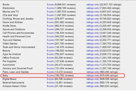
4 Experiment with Amazon Review Data 37 4.1 Amazon Product dataset. . . 37
4.2 Data Cleaning . . . 38
4.3 Word2vec and K-means . . . 40
4.4 Ranking Comments under a Real Amazon Product. . . 44
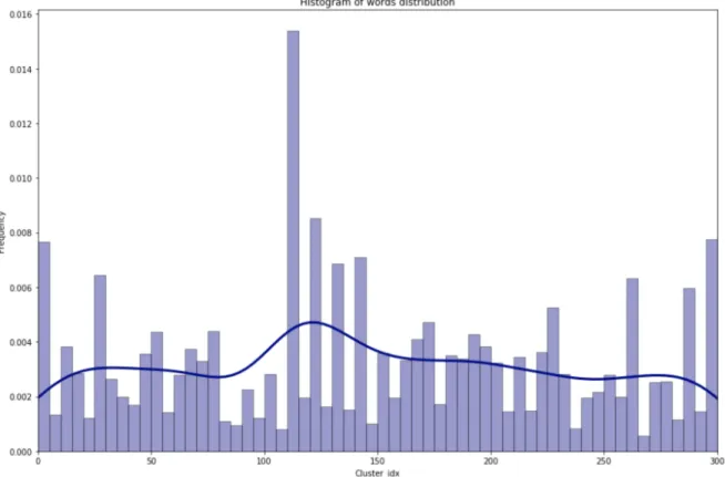
4.4.1 Global Word distribution . . . 44
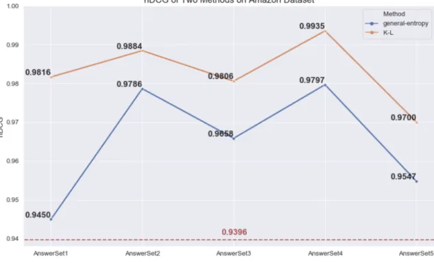
4.4.2 Ranking Performance . . . 46
4.4.3 Relationship Between K-L Divergence and the General Entropy . . . . 53
5 Conclusion 55 Bibliography 57 A Lists of Fake Comments 61 B Python Code 79 B.1 Data Cleaning . . . 79
B.2 word2vec model . . . 82
B.3 word embedding clustering . . . 84
B.4 Experiment with an Amazon Product . . . 85
Curriculum Vitae 86
List of Figures
2.1 Skip-gram model [24] . . . 15
2.2 Word2vec Example . . . 21
4.1 Amazon Product Dataset . . . 38
4.2 Amazon Data Sample . . . 38
4.3 Word2vec results . . . 41
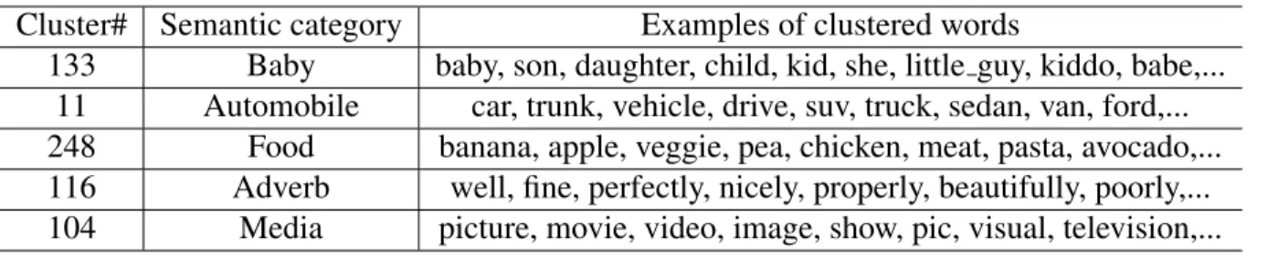
4.4 Product Detail [1]. . . 44
4.5 Global Word Distribution . . . 45
4.6 nDCG of Two Methods on Amazon Dataset . . . 47
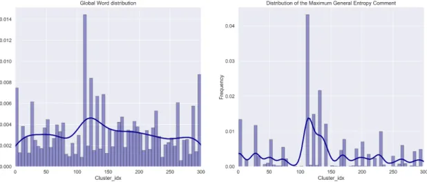
4.7 Global Distribution and the Maximum General Entropy Comment . . . 52
4.8 Relationship between General Entropy and K-L Divergence . . . 53
4.9 Distribution of the general entropy and K-L Divergence . . . 54
1.1 Example of Product Comments . . . 3
4.1 Example of Data Cleaning Process . . . 40
4.2 Parameters of Word2vec Model. . . 41
4.3 Examples of the word embedding clusters . . . 42
4.4 Examples of bag of word clusters representation . . . 43
4.5 Top 3 Most Frequent Word Clusters . . . 45
4.6 Top 3 Least Frequent Word Clusters . . . 46
4.7 Ranking Detail of Fake Comment Set 1 . . . 51
4.8 An Example of Comment with Low Complexity . . . 52
A.1 Detail of Fake Comment Set 2 . . . 65
A.2 Detail of Fake Comment Set 3 . . . 70
A.3 Detail of Fake Comment Set 4 . . . 74
A.4 Detail of Fake Comment Set 5 . . . 78
List of Appendices
Appendix A Lists of Fake Comments. . . 61
Appendix B Python Code . . . 79
Introduction
Nowadays, online shopping has become popular all over the world. The total spending of Canadian online shoppers reached $57.4 billion in 2018, compared to $18.9 billion in 2012, with nearly 84% of Internet users buying goods or services online, which means more than 8 in 10 Canadians shopped online [2]. There are many benefits of online shopping. The most obvious benefit of online shopping is convenience, shoppers can simply access online stores from their computer whenever they have free time available. Another benefit is that online shopping provides a greater diversity of products. This means you can choose goods that suit your requirements and budget the most. However, there are also disadvantages of online shopping. One of the most obvious ones is the lack of interactivity. You can not touch and feel the product you want to buy. Besides, the lack of touch and feel creates concerns over the quality of the product. For example, many people don’t like buying shoes online since people will not know if shoes fit unless they try it. With a large variety of goods and websites, people tend to do a lot of research before making a purchasing decision when doing online shopping. They will browse web pages about product details and, more importantly, check other buyer’s comments on the product site.
Gathering information based on other people’s opinions is an essential part of the purchas-ing decision process [8]. With the rapid growth of the Internet, these conversations in on-line markets provide a large amount of product information. So when doing onon-line shopping, consumers rely on online product comments, posted by other consumers, for their purchase decisions.
However, a large number of comments for a single product may make it harder for people to evaluate the true underlying quality of a product. In this situation, consumers tend to focus on the average rating of a product, like the number of stars on Amazon.com. But in reality, some products can easily obtain high average ratings by cheating while some other products may get unfair low ratings. Therefore, it is very important to extract these relevant and high-quality comments from the product site, which can help consumers obtain accurate information about this product.
1.1
How to judge a comment’s quality?
Before we start to construct a comment ranking algorithm, the fundamental question is how to judge a comment’s quality. Most online business sites evaluate their comments’ quality using criteria such as overall rating or helpfulness. Helpfulness is typically a score measured as the total votes given by consumers, which is an interesting way of defining a comment’s relevance and quality. Many researches in comments ranking area also use this type of helpfulness score as their comments’ evaluation score [32]. However, this method fails to identify these most recent comments with few votes. For example, we may always observe that only a few com-ments published a long time ago have a high helpfulness score in a product site, and most other comments have no votes. The reason for the phenomenon is that most people only read the first few pages of comments before making their purchase decisions. A new comment that has just appeared on the product site and has not received any votes until recently may remain at the bottom of the comment list. This comment may contain important information about this product, thus has the potential to rise to the top of the list.
There is also another type of comment’s quality evaluation method, Chen and Tseng [7] construct an information quality (IQ) framework for Internet product reviews. The IQ frame-work is a multi-dimensional frameframe-work in which each dimension represents a single aspect or construct of information items and is described by a set of features. Chen and Tseng treat each comment as an information item and construct fifty-one features from each comment, includ-ing the content of comments and believability of this product and comment authors’ reputation. Their framework is able to make a detailed comparison between each comment and also have
a good performance when ranking comments. However, their IQ framework requires too much information where most online business websites may not be able to provide, like authors’ rep-utation and product’s believability, and some of the features need human-annotated. Their IQ framework may not be feasible in most applications.
So how to judge each comment’s quality with only a collection of comments under a prod-uct? In our research, we judge each comments’ quality by theirrelevanceandtext complexity. We want to explain this by using an example. Table1.1below shows five comments of one of my favorite book “The Little Prince” on Amazon. It’s very easy for us to see that the first three comments have obviously better quality than the last two. Comment #4 has only two words “Fantastic book”, actually using these two words to describe this book is not inappropriate. So in terms of relevance, we can see that this comment is relevant to this product. However, in terms of text complexity, this comment is too concise and contains little information. Com-bining these two features together, we can easily see why this comment is not as good as the first three comments. Similarly, comment #5 is apparently an advertisement. In terms of text complexity, it’s better than comment #4 but forrelevance, it has almost no relevance to this product.
# Comment Helpfulness
1 One of the most influential books every read. Never forget the light of the child. It is spoken through so many true persons if “time” gone by.
2 2 I bought this book to read to my students. The story is very cute but
a little overwhelming with the underlying Concepts in the book. Al-though it is a story you can read to young children I would recommend waiting and having an older child read this book.
1
3 My favourite book arrived right on time. It has a folded corner but nothing that can’t be ignored. This is the best book in the world. It’s been written for little kids but has a lot of life lessons for us, the grown ups, who have forgotten about that kid that we once were. I highly recommend everyone to read it, at least once.
1
4 Fantastic book! 0
5 Please use this link http://bit.ly/125 to buy “wiki” book. 2 Table 1.1: Example of Product Comments
Relevance is a measure of how a comment is releted to this product andtext complexity
judge a comment’s quality.
1.2
Ranking Comments using Entropy
Ranking comments can be a very important task, and there is no doubt that there are many studies in this field. Some researches treat this ranking task as a supervised learning task, like [13] [3]. Most of them used the consumers’ votes, like helpfulness scores, as their training target. Then they adopted or designed several statistical or machine-learning models based on training data. As mentioned before, the reliability of this training data is hard to be assured; some high-quality comments may have relatively low votes. Moreover, these supervised rank-ing models can not be used on multiple products simultaneously since they have to be retrained for different products.
In this situation, we would like to develop a comment ranking algorithm that is unsuper-vised, which means we do not require any human-annotated training set. Besides, as we men-tioned before, in most cases, online business sites may not be able to provide some information, like the reviewer’s reputation. We prefer to develop an algorithm that ranks comments based on their contents. To construct this ranking algorithm, we need to solve these two problems below..
1. How to define a metric that can evaluate both comments’ relevance and text com-plexity?
2. How to effectively retrive information from comments’ content?
Let’s take a look at the first question first. When it comes to text complexity or informa-tion richness, we will naturally think of Shannon’s entropy [26]. In statistics, entropy is a quantity that can measure any random variable’s average rate of information inherent in the variable’s possible outcomes. For a discrete random variable X with all possible outcomes
{x1,x2, ...xm}and probability mass functionPX(x), the entropy is defined as,
H(X)= − m X i=1 PX(xi) logPX(xi)= m X i=1 PX(xi)IX(xi)=E[IX], (1.1)
as a random variable, thus entropy is actually expectation of self-informationIX. Self-information
can be regarded as the rate of information associated with one particular outcome of a random variable, and then entropy is the average rate of information of a random variable. To use entropy as a ranking metric, we need to consider each comment as a distribution of words, defined asP = [P0, ...,Pn], where nis the number of unique words andPi is the frequency of
ith words in this comment. There are different ways to represent a comment as a distribution, and we will describe later. Entropy is an effective measure of comment’s text complexity, Hsu et al [13] also used entropy as a comment complexity measure in their supervised comments ranking application. For example, if a comment only has one type of word in it like “good good good...good”, then this comment has a distribution withP(good)= 1, and the entropy of this comment is zero.
Take a look at the entropy formula again. We can see that this metric does not measure comment’s relevance to the product. So how to redefine entropy and take comment’s relevance into account? Zhang [31] defined a new entropy value called the general entropy. In his thesis, he developed an unsupervised ranking method on Amazon’s dataset and used the general entropy to measure the answer’s information quality. The general entropy is defined as follows.
E(P)=− n
X
i=0
Qi·Pi·logPi, (1.2)
whereP= [P0, ...,Pn] is the words distribution of an individual comment andQ=[Q0, ...,Qn]
is the distribution of the words of all comments combined under the same product, which is called global distribution. We can see that general entropy assigns weight on each self-information of word where the weight is the corresponding word probability in the global comment set. Since we want to measure the information richness and the relevance of a com-ment, we can give higher weight to these words that other comments also mentioned and lower weight to words that other comments hardly mentioned. More detail about this definition are described in Chapter 3.
The general entropy seems a good ranking metric that can measure both relevance and text complexity. However, in our experiment described in Chapter 4, comment with high com-plexity (for example, very long comment with many different kinds of words) and almost no
relevance to this product can get very high general entropy. These comments may have high ranks since most comments’ entropy scores are close to each other. So instead of calculat-ing scores for every comment, we first find an “ideal” comment and then judge comment by how far or how different it is from our “ideal” comment. Naturally, we can define comment with maximum general entropy as our “ideal” comment, and we call this “ideal” comment the
Maxmium General Entropy Comment. Since the maximum general entropy comment has the maximum general entropy, it keeps a good balance of relevance and information richness. We define theMaxmium General Entropy Commentas follows,
B=argmax
P
E(P). (1.3)
Note that the maximum entropy comment is a comment with the maximum general entropy within all possible comments. This comment may not exist in the existing comment set. Now, the question is how to measure each comment’ “distance” to this “ideal” comment. Since we treat each comment as a distribution, we can useKullback–Leibler (K-L) divergencedefined as follows, DKL(P|B)= n X i=0 Pi·log( Pi Bi ). (1.4)
Notice that this is a divergence, not a “distance”. Actually, K-L divergence is used to mea-sure how one probability distribution is different from others. In our application, we need to compare how each comment is different from the maximum general entropy comment. If a comment is similar to the maximum general entropy comment, it can get low divergence. Oth-erwise, if a comment is very different from the maximum general entropy comment, it may get high divergence. Compare to the method purely using the general entropy, this method achieved better performance in our experiment since it is more sensitive to comments’ rele-vance to the product.
1.3
Text Representation
Now, let’s consider the second problem described before: How to retrieve information from comments’ content effectively?. As we discussed in the previous section, in order to use entropy as our comments’ ranking metric, we need to treat each comment as a distribution of wordsP= [P1, ...,Pn]. Pis a numerical vector where each dimension indicates the frequency
of a word that appeared in the comment, andn indicates the number of unique words in the whole collection of comments. This is actually called the Bag of Words (BOW) model. A bag-of-words is a representation of text that describes the occurrence of words within a document. Despite the simplicity of this representation method, it has two significant disadvantages:
(1) the number of unique words in comments data is about 10000 while each comment has only 10-200 words, using the BOW model will lead to high-dimensional and sparse vectors.
(2) BOW representation doesn’t consider the semantic relation between words, it assumes all the words are independent. This assumption may have some problems, for example, “used bicycle” and “old bike” will be considered entirely different phrases because they have no words in common.
In Zhang’s research [31], he designed a new text representation method to solve these problems. In his method, firstly, he takes the maximum general entropy comment as a refer-ence to find “keywords” in the global comment set. Then he digitalizes each comment only considering these “keywords” and treats all other words as noise. For example, imagine we have a comment:
‘‘This is very easy to clean, very adjustable, and cute! Beautiful! This is the second one I have purchased."
And after data cleaning and removing stopwords, we have
‘‘easy-clean adjustable cute beautiful product second purchased".
Since the vocabulary size is normally far larger than the number of keywords selected, it’s possible that only “adjustable” and “product” are selected as keywords based on the maximum general entropy comment. It has seven words in total, then this comment can be digitalized as [17,17,57], the first two dimensions of this vector indicates two keywords “adjustable” and
“product” and the last dimension is the frequency of noise words. Finally, he will calculate each comment’s general entropy based on the frequency of these keywords and noise and rank comments based on their entropy value. This method can solve the BOW model’s sparsity problem, but it only considers a few keywords and treats other words as noise, which may lose a lot of information. In Zhang’s thesis, he also tried to solve the semantic relation problem of the BOW model. In his thesis, if two words represent the same meaning, he used one of them to replace another word. For example, he used “baby” to replace words like “diminutive”, “wee”, “babyish”, “tiny” and “youthful”. These synonyms are chosen based on a online dictionary called “thesaurus”. As we can see, this method can only partly solve the problem, one word may have multiple meanings in different situations. For example, using “baby” to replace every “tiny” in the comments is appropriate and may give the word “baby” an unrealistic high frequency.
In our thesis, we construct an entirely different method that can solve both the BOW model’s sparsity and semantic problem. We called our model: the bag of word clusters model. Unlike the traditional bag of words model that treats each word as an independent item, we group semantic-related words as clusters using pre-trained word2vec word embeddings [19] [20]. For example, consider the “used bike” and “old bicycle” example, we have four unique words: “old”, “bike”, “used” and “bicycle”. By using traditional BOW model, we can rep-resent “old bike” as vector [12,12,0,0] and represent “used bicycle” as [0,0,12,12]. As we can see, these two vectors are orthogonal, two vectors have no element in common, but in reality “used bicycle” and ”old bike” are semantic related. Using our methods, we will first group similar words like “bicycle” and “bike” into the same cluster and treat them as the same item. For example, we have two groups: cluster #1: “used”, “old”; cluster #2: “bike”, “bicycle”. Then we can represent “old bike” as [12, 12] where each dimension indicates one cluster, then the bag of word clusters representation of “used bicycle” is also [12,12]. Using this example, we can see that our method can solve the BOW model’s sparsity problem, the number of clus-ters is significantly smaller than the number of unique words. Also, we can retrieve semantic information from text, similar phrases “old bike” and “used bicycle” are represented as the same vector in our model. Besides, unlike Zhang’s method, which only considers keywords and treats all other words as noise, our method keeps most words and treats related words as
the same item. We believe our method can extract more information from text, thus has a bet-ter ranking performance. More detail about the bag of word clusbet-ters model is introduced in Chapter 2.
1.4
Thesis Outline
In this thesis, we propose a new unsupervised method to identify relevant comments under a product. There are several advantages of our ranking methods: a) it is entirely unsupervised, which requires no prior domain knowledge and no training data. Therefore, this method can be applied to most of the products’ comments ranking applications. b) This method is sensitive to the content of a comment and can successfully filter out unrelated comments. c) This method has low computational cost since it only requires statistical information from the text.
To help achieve better performance, in Chapter 2, we propose a new text representation method: the bag of word clusters model. Unlike the traditional bag of words model that treats each word as an independent item, we group semantic-related words as clusters using pre-trained word2vec word embeddings and represent each comment as a distribution of word clusters. This method can extract both semantic and statistical information from the text.
In Chapter 3, we give a detailed description of our ranking algorithm. Firstly, we introduced the general entropy, a ranking metric based on the Shannon entropy with respect to the global word distribution of a product’s comments. The general entropy is a simple metric that fo-cuses on both text complexity and relevance. Then, we develop an advanced algorithm that we first define the maximum general entropy comment as an “ideal” comment and rank comments based on their Kullback-Liebler (K-L) divergences to this “ideal” comment. This method is more sensitive to the relevance of the comments to the product and has a better ranking per-formance. Last but not least, we introduced our evaluation metrics: normalized Discounted Cumulative Gain (nDCG).
Chapter 4 introduces our experiment with a real Amazon product using the Amazon prod-uct dataset [12] [17]. We applied both pure general entropy and K-L divergence method on this product and K-L divergence method outperforms pure general entropy method in our ex-periment. By comparing these two methods, we can have a clear view on each method’s
char-acteristics and how they distinguish unrelated comments from actual comments. Moreover, we analyzed the relationship between the two ranking metrics of the general entropy method and K-L divergence method.
Bag of Words Model with Word
Embedding Clusters
In most text mining or text analytics applications, the first and fundamental problem is how we are going to represent text as input to our model or algorithm. More specifically, how to repre-sent the text documents to make them mathematically computable. Various text reprerepre-sentation methods were proposed during the last few years, the most commonly used text representation model in the area of text mining is called the Vector Space Model (VSM) [16], which aims to represent a text document as numerical vectors. One main advantage of VSM is that it is straightforward to compute the similarity between each vector (document), for example, by using cosine similarity.
One of the commonly used VSM is the Bag of Words model (BOW). A bag-of-words is a representation of text that describes the occurrence of words within a document. And to build a BOW model, people need to provide two things: the vocabulary of known words and a measure of the presence of known words. Given the document collectionD={di, i= 1,2,3...n}andm
unique words in these documents. Mathematically, each documentdican be represented by an m×1 vectorvi ∈Rm×1. For instance, consider there are three documents in this collectionD:
d1: I like learning text mining.
d2: What is text mining?
d3: Apple tastes good.
Now we can make a list of all words in our model’s vocabulary. The unique words here 11
(ignoring case and punctuation) are:{I,like,learning,text,mining,what,is,apple,taste,good}. As you can see, we have 10 unique words and 12 words in total within this collectionD.
The next step is to score each word in the documnet. There are many methods of scoring which we will discuss later. Let’s consider the simple Boolean first. If a word appears in a document, its corresponding weight is 1; otherwise, it is 0. Since our vocabulary has 10 words, we can use a fixed-length vector representation, with each position in the vector to score a word. Then the vector representations of these three documents are like this,
v1 =[1,1,1,1,1,0,0,0,0,0]
v2 =[0,0,0,1,1,1,1,0,0,0]
v3= [0,0,0,0,0,0,0,1,1,1],
notice that the order of word index is the same as the unique word list above.
The intuition of this model is that the information within a document is from its content, which are words in this case. Documents are similar if they have similar words in it. Since each of the three vectors has a fixed length, we can use cosine similarity to measure their similarity. Consider two vectorsA~andB~ with a fixed lengthN, cosine similarity is defined as follows,
Cosine S imilarity= A~·B~ ||A~||||B~|| = Pi=N i=1 AiBi q Pi=N i=1 A2i q Pi=N i=1 B2i , (2.1)
whereAiandBi are components of vectorsA~andB~, respectively.
The cosine value ranges between [−1,1], 1 for vectors pointing at the same direction, 0 for orthogonal, and -1 for vectors pointing in the opposite direction. For documents, the term values are usually non-negative, so the cosine similarity ranges between [0,1], the higher the value is, the more similar two documents are.
Now we can calculate the similarity between documentsd1,d2andd3 using this formula,
cos(d1,d2)=0.4472; cos(d1,d3)=0; cos(d2,d3)=0.
other because they are both talking about text mining, d3 has no relation withd1 and d2 thus
their cosine similarity is zero.
The BOW model is very straight forward and easy to implement. For the word weight in the BOW model, besides the simple Boolean model, we can also use counts of words, frequency or term frequency–inverse document frequency (tf-idf) as word weight, more information about this is referred to [25].
Despite the simplicity of this representation method, we will face two significant disadvan-tages if we want to adapt this method on our comments data: (1) the vocabulary size in com-ments data is about 10000 while each comment has only 10-200 words, using the BOW model will lead to high-dimensional and sparse vectors. (2) BOW representation doesn’t consider the semantic relation between words, it assumes all the words are independent. This assumption may have some problems, for example, “used bicycle” and “old bike” will be considered as entirely different phrases because they have no words in common.
In this chapter, we will develop a new text representation method based on the BOW model to overcome these disadvantages. Firstly, we will introduce word embeddings, a learned repre-sentation of words where words with the same meaning will have similar reprerepre-sentations [16]. Then we will introduce word2vec [19] [20], word2vec is a very effective algorithm to train word embeddings based on the local documents. With these word embeddings, we can easily group similar words as a cluster using the clustering method. Finally, instead of representing document (comment) as “bag of words”, we represent them as “bag of word clusters”. In this way, we can retrieve semantic information from the text, for example, “bike” and “bicycle” will be grouped together because they have the same meaning. Moreover, the BOW model’s sparsity problem will be handled since the number of clusters is significantly smaller than the vocabulary size.
2.1
Word2vec
Just like the BOW model, representing words as vectors is also a very essential topic in text mining and especially natural language processing area. With the increasing applications of machine learning and neural network in the natural language area, we need an efficient word
vectorization method that can represent word as vectors and also bring enough semantic infor-mation within the vector. Several methods are proposed during the last few years, and one of the most popular methods is word2vec.
Word2vec was created and published in 2013 by a team of researchers led by Tomas Mikolov at Google [19] [20]. Word2vec is a group of related models used to produce word vectors (also called word embeddings). Usually, word2vec can be referred to two model archi-tectures and two related training techniques:
- 2 model architectures: continuous bag-of-words (CBOW) and skip-gram(SG). CBOW aims to predict a center word from the surrounding context in terms of word vectors. Skip-gram does the opposite and predicts the probability of context words from a center word.
- 2 training techniques: negative sampling and hierarchical softmax. Negative sampling defines an objective by sampling negative examples, while hierarchical softmax defines an objective using an efficient tree structure to compute probabilities of appearance for all the vocabulary.
In our application, the skip-gram model with negative sampling will be used and introduced in this chapter, for a detailed explanation of other models in word2vec, one can refer to [24]. Moreover, since skip-gram is a neural network model, if you are not familiar with the neural network model, you can refer to [10].
2.1.1
Skip-gram
The basic idea of SG model is to predict context words based on a center word. More precisely, as in a sentence, our model is to take each current word as an input and predict words within a specific range before and after the current word. For example, we have the sentence “I am closing the window”, take the center word ”closing” as an input, the model will be able to predict the surrounding words: “I”, “am”, “the”, “window”. Generally, this model is a classifier on a binary prediction task: “is wordwilikely to appear near wordwjin a sentence?” However,
we do not care about the prediction task, and we will take the learned classifier weightsW as our word embeddings.
neural network with only one hidden layer. In our setting, the vocabulary size isV, and the hidden layer size isN. The units on adjacent layers are fully connected. The input is a one-hot encoded vector, which means for a given word wi in vocabulary, only the ith term in vector
[x1,x2,x3, ...xV] will be 1, and all the other terms are 0.
As you can see, there areC panels in the output layer, indicating the predicted multinomial distributions of C surrounding words of the input word. For example, yc,j is the predicted
probability of wordwj’s presence at positionc. Before training the model, you can arbitrarily
change the length of context windowCand the size of hidden layerN.
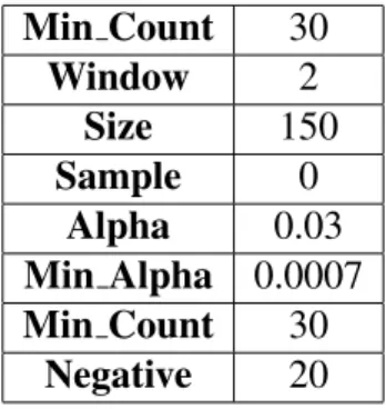
Figure 2.1: Skip-gram model [24]
As you can see from the Figure2.1, the weight matrix between the input layer and hidden layer is represented by aV × N matrixWV×N. Each row ofWV×N is the N-dimension vector
representation of the corresponding word of the input layer. Formally, we denote row i ofWV×N
asvwi
T. Given an input wordw
xwith xi∗ =1 and xj =0 for j,i∗, we have
h=WTx=WT(i∗,) := vw
I. (2.2)
So the hidden layer h = {hi}is simply copying a row of the weight matrix WV×N, which
means the link function between the input layer and the hidden layer is linear. From the hidden layer to the output layer, we have another weight matrixW0N×V, and all panels of the output
layer share the same weight matrix. For each position in the context of the input word, we can compute a score vectoruc,
uc =W0 Th,
(2.3) where c is from 1 toC. Then we denote jth column of W0N×V asv0wj, and each term of the
vectoruc would be,
uc,j =v0wj T
h= v0wj T
vwi. (2.4)
This is the score of wordwj at positionc, but not the final output. Remember the output
is the predicted probability of each word in the vocabulary at each position in the context, which is a multinomial distribution. Here we use the softmax function to convert each score to a probability, given the input word wI, the predicted probability of the word wj appear at
positioncis, ˆ P(wO,c =wj|wI)=yˆc,j = exp(uc,j) PV j0=1exp(uc,j0) , (2.5)
wherewO,cis the actual context word at positioncand ˆyc,j is the jthterm of the output panelc.
Substituting (2.4) into (2.5), we have
ˆ P(wO,c = wj|wI)=yˆc,j = exp(v0wj T vwI) PV j0=1exp(v0wj0TvwI) . (2.6)
From Mikolov, et al [20],vwandv0
ware called the “input” and “output” vector
representa-tion of wordw.
probability of observing actual output wordswO,1,wO,2, ...,wO,Cgiven the input center wordwI,
so the loss functionEis the negative log of this conditional probability (since we always want to minimize the loss function),
E= −log ˆp(wO,1,wO,2, ...,wO,C|wI) = −log C Y c=1 ˆ p(wO,c|wI) = −log C Y c=1 exp(uc,j∗c) PV j0=1exp(uc,j0) = − C X c=1 uc,j∗ c + C X c=1 log V X j0=1 exp(uc,j0), (2.7) where j∗
c is the index of the actual c-th output context word in the vocabulary, notice that this
model makes a very strong assumption that all context words in different positions are inde-pendent of each other. With the loss functionEdefined, we can now derive the update equation for the weight matrix in the model. Here we used a training technique called backpropagation, which in general is to update weight backward. In our case, it is to update hidden→output matrixW0 first, then update input→hidden matrixW, for more detail about backpropagation, please refer to [10].
First, let us derive the gradient of the loss function with respect to output scoreuc,j, ∂E
∂uc,j
= yˆc,j−yc,j := ec,j, (2.8)
where yc,j will be 1 if j is the index of the actual output word and 0 otherwise, note that the
derivative is simply the prediction errorec,j.
Now let us denote each component ofW0 asω0
i j, by using the chain rule, we can obtain the
gradient ofEwith regard toω0i j,
∂E ∂ω0 i j = C X c=1 ∂E ∂uc,j · ∂uc,j ∂ω0 i j = C X c=1 ec,j·hi. (2.9)
Then with learning rate ηwe can have the update equation for hidden layer→output layer weight matrixW0,
ω0(new) i j =ω 0(old) i j −η· C X c=1 ec,j·hi (2.10) or v0w(jnew)= v 0(old) wj −η· C X c=1 ec,j·h. (2.11)
(2.11) is the update equation for the output vector. Now we can move to the input→hidden matrixW, first we take derivative of Eon hidden layerhi,
∂E ∂hi = V X j=1 C X c=1 ∂E ∂uc,j · ∂uc,j ∂hi = V X j=1 C X c=1 ec,j·ω0i j (2.12)
and takexkas thekthunit of the input layer, using the chain rule again, the derivative ofhiwith
respect to each element ofWis
∂E ∂ωki = ∂E ∂hi · ∂hi ∂ωki = V X j=1 C X c=1 ec,j·ω0i j· xk. (2.13)
Remember the input xis a one-hot encoded vector, only one component is 1, and all the others are 0. So at each iteration, only one row of the weight matrixWwill be updated, which is the ”input vector”vwI, and the update equation is
v(wnew) I =v
(old)
wI −η·EH, (2.14)
whereEHis a N-dimensional vector with each elementEHi is defined as
EHi = V X j=1 C X c=1 ec,j ·ω0i j. (2.15)
Now we have already obtained the update equation ofWandW0, when training this model,
at each iteration, the output matrix W0 will be update first using equation (2.11) and then we use the updated matrixW0(new)to update matrixWby using equation (2.14). Normally, we use
2.1.2
Negative sampling
In the previous section, we discussed the original form of the skip-gram model without any optimization techniques. As you can see, there is a problem with the update equation (2.11): its computational complexity is too large. During training process, for each training iteration, it will scan all the wordswj in the vocabulary and compute its predicted probability and error.
Since there are C context words, the computational complexity will be O(C ×V) while the vocabulary sizeV can go easily beyond 104. Doing such computation at each iteration is very expensive. And to get a high-quality vector representation of words, the model needs to be trained on a large amount of text data.
To fix this problem, Mikolov et al. proposed a method in [20] called negative sampling. Instead of updating every output vectors at each iteration, we only update a sample of them. Of course, we will keep these positive sampleswc,j∗c in our sample set and randomly select a few
words in the vocabulary as negative samples.
Before training, people can determine a distribution themselves for sampling negative sam-ples, in Mikolov et al.’s paper [20], they used a unigram distribution:
Pα(w)= count(w) α
P
w0count(w0)α
, (2.16)
whereαis commonly set as 0.75. We can chooseknoise words for every postioncaccording to this distribution, and these groups of noise words are denoted asWc,neg ={wc,j|j=1,2,3, ...,k}.
For the loss function E, instead of using a multinomial distribution like 2.7, Mikolov et al defined a simplified loss function,
E = − C X c=1 logσ(uc,j∗ c)− C X c=1 X j0∈W c,neg logσ(−uc,j0), (2.17)
whereσ(x)= 1+1e−x is a sigmoid function. To obtain the update equation, let’s first take
∂E ∂uc,j = σ(uc,j)−1, i f wc,j =wc,j∗ c σ(uc,j), i f wc,j ∈Wc,neg 0, otherwise (2.18) = σ(uc,j)−yc,j, i f wc,j ∈ {wc,j∗c} ∪Wc,neg 0, otherwise . (2.19) Remember thatwc,j∗
c is the actualcthoutput context word andyc,jequals to 1 only if j= j
∗
c
and equals to 0 otherwise. Now we can obtain the update equation for the output vector,
∂E ∂v0 wj = C X c=1 ∂E ∂uc,j · ∂uc,j ∂v0 wj = PC c=1(σ(uc,j)−yc,j)·h i f wc,j ∈ {wc,j∗ c} ∪Wc,neg 0 otherwise (2.20) v0w(jnew) = v0w(jold)−η· PC c=1(σ(uc,j)−yc,j)·h i f wc,j ∈ {wc,j∗c} ∪Wc,neg v0w(jold) otherwise , (2.21)
as you can see, we only need to update vectors of wc,j ∈ {wc,j∗
c} ∪Wc,neg, while other output
vectors will remain the same. So the computational complexity per iteration will be reduced fromO(C×V) toO(C×k) wherekusually ranges from 5 to 20.
2.2
Word Embedding clusters with K-means
Training using word2vec model produces N-dimensional vectors for each word in our vocab-ulary. These word embeddings have many good properties that we can use. Since each word embeddings have the same sizeN, it is easy to measure the distance between a pair of word em-beddings. Another property of these pre-tained word embeddings is that semantically related words usually have a close distance. Here we use the cosine similarity defined at (2.1), and the more similar two words are the higher cosine similarity of their word embeddings. Fig2.2are three examples of words “baby” “apple” and “well” with their top 10 most similar words in
the whole vocabulary with around 104 words. More detail about how these word embeddings trained is described in Chapter 4.
Figure 2.2: Word2vec Example
As you can see, the most similar words calculated by cosine similarity are very similar to the target words, for example, “child”, “babe”, “infant”, “little guy” are indeed very similar with target word “baby”. The top 10 most similar words of “apple” are all fruit or vegetables. And what’s more surprising is that these most similar words are not just semantically related with target words but also syntactically. In the most similar words of “well”, most of the words are adverbs.
As we mentioned before, instead of treating each word as an independent term, we prefer to group similar words as a cluster and treat the words in the same cluster as the same term. Here we need a clustering method to be able to put similar words in the same group as well as keep not similar words in different groups.
The clustering of word embedding is actually applied to various studies. Gonzalez et al. [21] developed a system to extract mentions of adverse drug reactions (ADRs) from the highly informal text in social media. In their model, by grouping word embeddings using k-means, they can assign the same cluster number to similar words as a feature that adds a higher-level abstraction to the feature space. Wang et al. [28] constructed a convolutional neural network
(CNN) for short text classification and used word embedding clusters as a feature extension.
2.2.1
K-means Algorithm
In our method, we adopt the K-means algorithm [11] to perform word embeddings clustering. K-means is a straightforward and efficient algorithm for general clustering. We will introduce how k-means are applied in our method, let us review this algorithm first.
In this clustering problem, we are givennword embeddings as our training set{w(1),w(2), ...,w(n)}
andw(i) ∈
RN. The number of clusters is a pre-set parameterK, and the K-means algorithm are
as follows:
1. Initialize cluster centroidsµ1, µ2, ..., µK ∈RN randomly;
2. Repeat until convergence: {
for everyi∈ {1, ...,n}, set
c(i) :=arg min
j ||w
(i)−µ
j||2 (2.22)
for every j∈ {1, ...,K}, set
µj = Pn i=11{c( i)= j}w(i) Pn i=11{c(i)= j} (2.23) }
For every repetition, there are two steps, first is to assign each training sample w(i) to its nearest cluster µj and update its assigned cluster index ci. Then, update the clusterµ
j to the
mean of the points assigned to it. The K-means algorithm can also be regarded as a coordinate descent on the distortion functionJ,
J(c, µ)=
n
X
i=1
||w(i)−µc(i)||2. (2.24)
As you can see, the distortion function is a non-convex function, so the K-means algorithm can easily get stuck in local minima. One common solution to this problem is to run K-means many times with different random initialization ofµand out of all different clusters founded, use the one with the lowest distortionJas our final solution.
we mentioned before, but K-means use only Euclidean distance as the distance measure. Al-though other clustering methods can use cosine as a distance measure like K-medoids [15], we still use K-means due to its much higher computational efficiency. And we can justify that for normalized vectors, cosine similarity and Euclidean distance are linearly connected. For two normalized vectors A = {Ai}, B = {Bi}(PA2i =
P
B2i = 1), the Euclidean distance between A
andBis ||A−B||2= X(Ai−Bi)2 = X (A2i +B2i −2AiBi) = X A2i + X B2i −2 X AiBi = 1+1−2 cos(A,B) = 2(1−cos(A,B)). (2.25)
Note that for normalized vectors cos(A,B) = √ PAiBi
P A2i √ P B2i = P
AiBi. The higher two word
embeddings’ cosine similarity is, the closer their Euclidean distance is, which is consistent with our objective. Thus in our application, we will perform k-means on the normalized pre-trained word embeddings.
2.2.2
Bag of word clusters representation
As we discussed at the beginning of this chapter, instead of representing text documents as “bag of words”, we would like to represent them as “bag of word clusters”. Now we have our pre-trained word embeddings, and then we perform K-means algorithm, which assigns each word a unique cluster index. Then constructing bag of word clusters representation of text document can be summarized as the following steps:
1. Preprocess and tokenize the text (see Chapter 4 for more detail of data preprocess), then each text will be represented as a list of words;
2. Given pre-trainedKword cluster, replace each word in the list as its cluster index, if there are unknown words, replace them with K+1, so this vector will be transformed to numerical lists with the number 1 toK+1;
where each term will be the calculated frequency of clusters with the corresponding index number. And this new vector is our “bag of clusters” representation of text.
As you can see, we will be able to transform each text into aK+1-dimensional vector. For example, we have a short text:
‘‘I love eating apples, they are delicious"
and we have four pretrained word clusters:C1 = {“I”,“they”,“you”},C2 ={“apple”,“pear”,
“banana”},C3 = {“is”,“are”,“was”},C4 = {“delicious”,“good”,“tasty”}. First, we tokenize
this text as a vector v = [“I”,“love”,“eating”,“apples”,“they”,“are”,“delicious”], then re-place these words with corresponding clusters v = [1,5,5,2,1,3,4], remember to replace unknown words with ”k+1” which is 5 here. Next we calculate each cluster’s relative fre-quency: f1 = 27, f2 = 17, f3 = 17, f4 = 17, f5 = 27, and represent this text with new vector
v0 =[f
1, f2, f3, f4, f5]=[27,17,17,17,27].
Text digitalization or representing text as numerical vectors is an essential part of every text mining application. Our “bag of word clusters” model can extract not only statistical information but also part of semantic information from text.
Ranking comments with general entropy
In this chapter, we will introduce our comment ranking method. Firstly, we will introduce
General Entropy [31] and how to rank comments directly based on the entropy value. Then we will introduce theMaximum Entropy Comment, by treating the maximum entropy com-ment as an ”ideal” comcom-ment, we can measure each comcom-ments distance to the ”ideal” comcom-ment by using K-L divergence and rank comments based on this distance. Moreover, there are two features of our comment ranking algorithm:
1) Our method is unsupervised, which means there is no human-labeled training set we can learn from, all we have is a group of comments without any order. In other words, our method does not depend on an annotated training set;
2) Judging the quality of a comment is subjective, and we can’t just create a judgement standard from nothing. So the objective of our method is not to distinguish these top-ranked comments but to make sure those unrelated or “fake” comments have as lower ranks as possi-ble. In general, one of the objectives of our method is to filter out “bad” comments.
Ranking comments can be a very important task. As the internet develops fast, people tend to get information from these comments on websites, for example, when doing online shopping, people always like to check the comments of a product and these comments have a great influence on their decisions. So there is no doubt that there are many studies in this field. Chiao-Fang Hsu et al [13] proposed a machine learning based approach for ranking comments on the social Web. They extract several different features from each comment: comment visibility, user reputation and content-based features, in the content-based features,
they also used entropy as a comment complexity measure. Since the comment data they used have already been ranked by community ratings (for example, the number of “likes”), they treat this ranking problem as a regression problem where the objectiveyis community ratings. Burges et al. [6] designed a cost function for the ranking problem and constructed a neural network model, Ranknet. This model is simple to train and has excellent performance with a large amount of data. Tulio et al. [3] developed an application to filter out spam comments on youtube called TubeSpam. They vectorized each comment using the BOW model with term weight as term frequency and used these vector as input to their model. Their study compared several different machine learning models like decision tree, SVM, knn, etc. In their application, the Bernoulli Naive Bayes model is chosen since it offered a good balance between robustness and computational effort.
We learned a lot from these studies about how they extract information from these com-ments. However, most of them used a supervised learning technique with a large amount of pre-classified data. There are also some researches about unsupervised text ranking, but not as many as the supervised ones. Rada and Paul proposed TextRank [18], a graph-based model for text processing. This model’s objective is to extract keywords and key sentences from a long document, which is also called text summarization. For key sentence extraction, each sentence will be the node of this graph model and fully connectedto each other, and the transition prob-ability between each node is the calculated similarity between sentences. After setting up the graph model, they let computer simulate traversing the whole graph and calculate the score of each sentence. At last, sentences with high scores will be extracted as key sentences. This algorithm is motivated by Google’s PageRank [5] and perform well on long documents like research papers. Vinicius et al. [29] proposed MRR (Most Relevant Reviews), an unsuper-vised algorithm that identifies relevant reviews based on the concept of graph centrality. The intuition behind this approach is that central reviews highlight aspects of a product that many other reviews frequently mention. MRR is a graphic model where vertices represent reviews connected by edges and each edge is the similarity between a pair of reviews. Then reviews are ranked with the centrality scores calculated by the PageRank algorithm.
The graphic model like TextRank is state of the art in unsupervised text ranking area. How-ever, the graphic model focuses more on the relevance or similarity between each pair of
com-ments. In our methods, we focus more on comments information quality as well as its relevance to the whole group of comments under a specific product.
General Entropy was first introduced by Zhang [31], he developed a ranking method on Amazon’s question-answering dataset and used general entropy as a measure of answer’s in-formation quality. However, he has an entirely different text digitalization method with us, he only considered each word’s frequency in the document and chose some of the most fre-quent words as keywords while all other words as noise. His method can also solve the high-dimension problem of text digitalization but did not extract semantic information from text. For example, under a food product, most comments described this food as “delicious”, only a few of them used the word “tasty”. If we treat high-frequency word ”delicious” as keyword and low-frequency word “tasty” as noise word, then comments using ”delicious” will be considered having higher information quality than comments using “tasty”, which is not reasonable. While in our digitalization method, we will group similar words like “delicious” and “tasty” and treat them as the same item. There are also other differences in terms of the ranking algorithm, and we will discuss them later in this chapter.
3.1
General Entropy
After the pre-trained word embedding clustering, givenn clusters of words andmcomments under a product, we regard the collection of allmcomments together as theGlobal Comments Set. Then we can calculate the number of each word cluster appears in the global comments set, which can be represented as{NumG0,NumG1,NumG2, ...,NumGn}, notice thatNum
G
0 is the number
of unknown words that appear in the collection. Now we can define theglobal probabilityof word clusteriin the global comments set as,
Qi =
NumGi
NumG0 +NumG1 +NumG2 +...+NumG n
. (3.1)
And for all global probabilities, we have
n
X
i=0
Remember that in Chapter 2, to ensure these word embeddings’ quality, our word2vec model has to be trained on a large corpus with around 104-105 unique words. Then we can
group these words intonword clusters. One feature of our bag of word clusters model is that these pre-trained word clusters can be used for many products at the same time. So for one product, it’s possible that no word within its global comments set falls into the word clusteri∗. In other words, it’s possible that global probabilityQi∗ = 0 for this product.
In our comments ranking method, we tend to treat each text or comment as a distribution of word clusters. If two comments have similar distributions, they probably expressed similar meanings. And as an unsupervised method, without any training set, the global comments set’s distribution can be an essential reference for determining each individual comment’s relevance to others. We believe that under a product, most comments will focus on some specific as-pects of this product, which tend to have similar distributions of words, if a comment have a completely different word distribution with the others, it might be a “fake comment.”
The same as global probability, for an individual comment with index j, we have the num-ber of each word cluster in the comment as{Num0j,Num1j,Num2j, ...,Numnj}, the probability of
word clusteriin the jthcomment can be defined as,
Pij = Num
j i
Num0j +Num1j+Num2j +...+Numnj
, (3.3) where n X i=0 Pij =1, (3.4)
note thati f Qi = 0 thenP j i =0.
As we mentioned in Chapter 2, each comment including the global comments set can be represented by an+1 dimensional vector, with our new definition, for global comment set, the vector is [Q0,Q1,Q2, ...,Qn] and for individual comment j is [P
j 0,P j 1,P j 2, ...,P j n]. By treating
each comment as a distribution, we can assess each comment’s information quality by calcu-lating entropy based on these probabilities.
In statistics, entropy is a quantity that can measure any random variable’s average rate of information inherent in the variable’s possible outcomes, and the concept of entropy was
first introduced by Claude Shannon [26]. For a discrete random variable X with all possible outcomes{x1,x2, ...xm}and probability mass functionPX(x), the entropy is defined as,
H(X)= − m X i=1 PX(xi) logPX(xi)= m X i=1 PX(xi)IX(xi)=E[IX], (3.5)
whereIX(xi) is self-information associated with outcome xi. We can treatIX(xi)= −logPX(xi)
as a random variable, thus entropy is actually expectation of self-informationIX. Self-information
can be regarded as the rate of information associated with one particular outcome of a random variable, then entropy is the average rate of information of a random variable. As you can see, self-information IX(xi) is simply a negative log of the probability of this event, and this
is monotonically decreasing in probability PX(xi). To help understand self-information, take
a simple example, imagine a person randomly select a book from a library, and he observes that the word “the” is in this book. This observation hardly gives him any information since the word “the” has a very high probability appearing in any document. However, if he observes the word “Shakespeare” in that book, he may learn that the book might relate to literature or po-etry. The word “Shakespeare” has a lower probability appearing in a book, and this observation definitely contains more information than the last one.
In terms of comments, we treat each comment as a multinomial distribution of word clus-ters with probabilityPj = [P0j,P1j,P2j, ...,Pnj], that is if we randomly sample a word from this
comment, this word should have this probability distribution. For the worst scenario, if a com-ment only has one type of word in it like “good good good...good”, then this comcom-ment has a distribution withP(good) = 1, and the entropy of this comment is zero. For the best scenario, without any constraint, the uniform distribution is the maximum entropy probability distribu-tion for a random variable. The reason is that the entropy score is the “expected informadistribu-tion gain” and the hardest distribution to predict is the uniform distribution when using a binomial score. [30]. For example, if a comment has an equal probability of every word cluster in it, it would have the maximum entropy. However, if we use entropy defined at (3.3) as our ranking score, a comment with uniform distribution would rank highest under any product, which can-not be used in our application. That is why we have to consider each comment relevance to the others, so we define theGeneral Entropyas follows,
Definition 1 (General Entropy) Given global probability Q = {Q0,Q1, ...,Qn} and a com-ment with probabilityPj ={Pj
0,P
j
1, ...,P
j
n}, the general entropy of this comment is
E(Pj)= − n X i=0,Pij,0 Qi·P j i ·logP j i.
Notice that Pij can be 0 since a comment may not include all word clusters. The general entropy can measure the average information rate for an individual comment j with respect to the global probability. From the entropy definition at 1, we can see that general entropy assigns weight on each self-information of word cluster where the weight is the corresponding global probability. As we mentioned before, the global probability can be regarded as a high-level abstraction of the topic in the comments under this product. Since we want to measure the information richness and the relevance of a comment, we can give higher weight to these words that other comments also mentioned and lower weight to words that other comments hardly mentioned.
At last, we can summarize our general entropy ranking algorithm as follows:
Algorithm 1Ranking comments based on the general entropy
Input:
The set ofnword clusters;
The set ofmcomments under a product;
Output:
Ranking results of all comments;
1: Covert all comments into their bag of word clusters representations;
2: Calculate the global probabilityQ=[Q0,Q1,Q2, ...,Qn];
3: Calculate each comment’s probability: Pj = [P0j,P1j,P2j, ...,Pnj], j=1,2...m;
4: Calculate each comment’s general entropyE(Pj);
5: Rank comments based on their general entropy, comment with higher general entropy is ranked higher;
3.2
Kullback–Leibler (K-L) divergence to the Maximum
Gen-eral Entropy Comment
In the previous section, we introduced the general entropy, which simultaneously measures information richness and relevance of a comment. However, in our experiment, comment with high complexity (for example, very long comment with many different kinds of words) and almost no relevance to this product can get pretty high general entropy. These comments may have high ranks since most comments’ entropy scores are close to each other. So instead of calculating scores for every comment, we first find an “ideal” comment and then judge comment by how far or how different it is from our “ideal” comment. Naturally, we can define comment with maximum general entropy as our “ideal” comment, and we call this “ideal” comment the Maxmium General Entropy Comment. Since the maximum general entropy comment has the maximum general entropy, it keeps a good balance of relevance and information richness. We define theMaxmium General Entropy Commentas follows,
Definition 2 (Maxmium General Entropy Comment) Given global probabilityQ= {Q0,Q1,
...,Qn}, the maximum general entropy commentB:={B0,B1, ...,Bn}are defined as
B=argmax
P
E(P),
whereP:={P0,P1, ...,Pn}andPni=0Pi = 1.
Note that the maximum entropy comment is a comment with the maximum general en-tropy within all possible comments. This comment may not exist in the existing comment set. However, it can be regarded as a standard to judge each comment’s relevance to the product. The following theorem shows that the maximum entropy comment exists and is unique, given a collection of comments.
Theorem 3.2.1 Given gloabl probabilityQ = {Q0,Q1, ...,Qn}and an index set C that i ∈ C if Qi , 0 and i < C otherwise. Then there exist an unique maximum general entropy answer B = {B0,B1, ...,Bn}so thatB = argmaxPE(P)and Bi =
e−1−Qiλ i∈C 0 i<C , whereλis a unique
value andPn
i=0Bi = 1.
Proof Fori<C,Qi =0, which means word clusters with indexinever appear in the collection
of all comments. Then for any comments in the collections,Pij =0 fori<C and j=1,2, ...m.
Since we would like to compare each comment in the collections with the maximum entropy comment, we determine allBi = 0 fori<C.
Fori∈C, in order to maximizeE(P), we define the objective function f as,
f(P0,P1, ...,Pn, λ)=−
X
i∈C
Qi ·Pi·logPi+λ(1−P0−P1−...−Pn),
whereλis the Lagrange multiplier.
Take the derivative of f with respect toPi ∂f
∂Pi
=−Qi−Qi·logPi−λ =−(1+logPi)Qi−λ,
then set the derivative to 0,
−(1+logPi)Qi−λ=0.
We have the solution to the equation above, ˆ
Pi =e
−1−λ
Qi f or i∈C. (3.6)
Assume we have more than one element in set C, to solve λ, we have two conditions 1> Pˆi >0 and
Pn
i=0Pˆi =1. Based on the first condition,
for alli∈C,
1> Pˆi >0.
ˆ
Piis exponential thus bigger than 0, then for anyi∈C,
ˆ
Pi = e
−1−λ
Take logarithm on both sides, 1+ λ Qi >0, then, λ >−Qi.
Since this inequality holds for allQi, to conclude, we have
λ >−min{Qi|i∈C}. (3.7)
Based on the second condition, we set the objective function
g(λ)= n X i=0 ˆ Pi−1 =X i∈C e−1−Qiλ −1.
Taking the derivative ofgwith respect toλ,
∂g ∂λ =− X i∈C 1 Qi ·e−1− λ Qi.
The derivative ofgis negative forλ >−min{Qi|i∈C}which meansgis monotone
decreas-ing function, then we have
lim
λ→−min{Qi|i∈C}
g(λ)> 0and lim
λ→∞g(λ)=−1.
Thus the solution ofλis unique.
In conclusion, we have the maximum general entropy comment Bi =
e−1−Qiλ i∈C 0 i<C ,
whereλis a unique value .
After the definition of the “ideal” comment, now we need a method to measure each com-ment’s distance to the maximum general entropy comment. As we mentioned before, we treat each comment as a multinomial distribution with probability {P0j,P1j, ...,Pnj}, that is if we
Pij. We treat the maximum general entropy answer the same way, the maximum general en-tropy answer is a multinomial distribution with{B0j,B1j, ...,Bnj}, to measure how one probability
distribution is different from others, we use Kullback–Leibler (K-L) divergence define as follows,
Definition 3 (Kullback–Leibler (K-L) divergence) Given jth comment probabilityPj = {Pj
0,
P1j, ...,Pnj}and the maximum general entropy commentB={B0,B1, ...,Bn}, the Kullback–Leibler divergence from the maximum general entropy commentBto jth commentPj is defined to be
DKL(Pj|B)= n X i=0,Pj i,0 Pij·log(P j i Bi ).
In statistics, we call B the prior probability distribution and Pj the posterior probability distribution, and the K-L divergence fromBtoPjis,
DKL(Pj|B)= n X i=0,Pij,0 Pij·log(P j i Bi ) = − n X i=1,Pij,0 Pij·log(Bi)−(− n X i=1,Pij,0 Pij·log(Pij)) = − n X i=1,Pj i,0 Pij·log(Bi)−H(Pj). (3.8)
According to the entropy defination at (3.5), DKL(Pj|B) is actually the information gain if
we use distribution Bto approximatePj. When two distributions are close to each other, this
value can be relatively small, and large if two distributions are very different. The first item
−Pn
i=1,Pij,0P
j
i ·log(Bi) in (3.8) are calledcross-entropy, which is a very popular loss function
of classification problem in machine learning area.
Algorithm 2 Ranking comments based on K-L divergence to the maximum general entropy comment
Input:
The set ofnword clusters;
The set ofmcomments under a product;
Output:
Ranking results of all comments;
1: Covert all comments into their bag of word clusters representations;
2: Calculate the global probability: Q=[Q0,Q1,Q2, ...,Qn];
3: Calculate each comment’s probability: Pj =
[P0j,P1j,P2j, ...,Pnj], j=1,2...m;
4: Based on the global probability Q, find the maximum general entropy comment: B = {B0,B1, ...,Bn};
5: Calculate each comment’s K-L divergence to the maximum general entropy commentB;
6: Rank comments based on their K-L divergence, comment with lower divergence is ranked higher;
7: return Ranking results.
3.3
Evaluate Ranking Quality with nDCG
In the previous section, we introduced our new comment ranking algorithm, naturally, the next step is to assess this algorithm by evaluating the ranking quality. Here we introduce normal-ized Discounted Cumulative Gain (nDCG) [14], it is often used to measure the effectiveness of web search engine algorithms, but it can also applied to text ranking application. Many re-search mentioned before [13] [29] adapt this method to assess their ranking algorithm. Firstly, let us defineDiscounted Cumlative Gain (DCG).
Definition 4 (Discounted Cumlative Gain (DCG)) Given a ranked list with m comments, and reli is graded relevance of the result at position i, Discounted Cumulative Gain is defined as
DCGm= m X i=1 reli log2(i+1).
According to this definition, if a comment with high graded relevance appears lower in the ranking result, it will be penalized as the graded relevance value is reduced logarithmically proportional to the position of the ranking result. To achieve high DCG value, the algorithm should rank a high relevance comment higher than low relevance one. Notice that in our
application, graded relevance reli is a manually annotated comment quality score that will
not be used as an input in our algorithm, more detail about our experiment are described in Chapter 4.
While DCG is already a valid measure of ranking quality, it does not have a proper upper and lower bound to let people better compare the performance of different ranking results, then
normalized Discounted Cumulative Gain (nDCG)is defined as follows,
Definition 5 (normalized Discounted Cumulative Gain (nDCG)) Given a ranked list with m comments and its DCG value, the normalized Discounted Cumulative Gain is computed as,
nDCGm =
DCGm IDCGm
, where IDCGmis the Ideal Discounted Cumulative Gain.
IDCGm is straightforward to compute where the ideal ranking result is to rank these
com-ments directly based on their graded relevance. nDCG ranges from 0 to 1 while 0 will not be able to achieve, and the closer our nDCG is to 1, the better quality our result has.
Experiment with Amazon Review Data
In this chapter, we will introduce our experiment built on the Amazon product dataset [12] [17], which contain
![Figure 2.1: Skip-gram model [24]](https://thumb-us.123doks.com/thumbv2/123dok_us/741222.2593849/24.918.305.651.443.828/figure-skip-gram-model.webp)
![Figure 4.4: Product Detail [1]](https://thumb-us.123doks.com/thumbv2/123dok_us/741222.2593849/53.918.112.781.368.683/figure-product-detail.webp)