Physically inspired methods
and development of data–driven
predictive systems
by
Marcin Budka
A thesis submitted in partial fulfilment for the degree of Doctor of Philosophy
School of Design, Engineering & Computing Bournemouth University
This copy of the thesis has been supplied on condition that anyone who consults it is understood to recognise that its copyright rests with its author and due acknowledgement must always be made of the use of any material contained in, or derived from, this thesis.
Traditionally building of predictive models is perceived as a combination of both science and art. Although the designer of a predictive system effectively follows a prescribed procedure, his domain knowledge as well as expertise and intuition in the field of machine learning are often irreplaceable. However, in many practical situations it is possible to build well–performing predictive systems by following a rigorous methodology and offsetting not only the lack of domain knowledge but also partial lack of expertise and intuition, by computational power. The generalised predictive model development cycle discussed in this thesis is an example of such methodology, which despite being computationally expensive, has been successfully applied to real–world problems.
The proposed predictive system design cycle is a purely data–driven approach. The quality of data used to build the system is thus of crucial importance. In practice however, the data is rarely perfect. Common problems include missing values, high dimensionality or very limited amount of labelled exemplars. In order to address these issues, this work investigated and exploited inspirations coming from physics. The novel use of well–established physical models in the form of potential fields, has resulted in derivation of a comprehensive Electrostatic Field Classification Framework for supervised and semi–supervised learning from incomplete data.
Although the computational power constantly becomes cheaper and more accessible, it is not infinite. Therefore efficient techniques able to exploit finite amount of predictive information content of the data and limit the computational requirements of the resource–hungry predictive system design procedure are very desirable. In designing such techniques this work once again investigated and exploited inspirations coming from physics. By using an analogy with a set of interacting particles and the resulting Information Theoretic Learning framework, the Density Preserving Sampling technique has been derived. This technique acts as a computationally efficient alternative for cross–validation, which fits well within the proposed methodology.
All methods derived in this thesis have been thoroughly tested on a number of benchmark datasets. The proposed generalised predictive model design cycle has been successfully applied to two real–world environmental problems, in which a comparative study of Density Preserving Sampling and cross–validation has also been performed confirming great potential of the proposed methods.
Abstract III List of figures IV List of tables V Acknowledgements VII List of abbreviations IX Notation IX 1 Introduction 1 1.1 Background . . . 1
1.2 Project description and goals . . . 3
1.3 Original contributions and publications resulting from this work . . . 4
1.4 Organisation of the thesis . . . 5
2 Machine learning and physically inspired techniques 7 2.1 Introduction . . . 7
2.2 Designing a predictive system . . . 8
2.2.1 Classical predictive system design cycle . . . 9
2.2.2 Generalised predictive system design cycle . . . 11
2.3 Physically inspired learning . . . 21
2.3.1 Data field models . . . 22
2.3.2 Information Theoretic Learning . . . 25
2.4 Concluding remarks . . . 28
3 Electrostatic Field Classification Framework for incomplete data 30 3.1 Introduction . . . 30
3.2 Data field classifiers . . . 31
3.2.1 Gravity Field Classifier . . . 31
3.2.2 Electrostatic Field Classifier . . . 32
3.3 Improvements of the original Electrostatic Field Classifier . . . 33
3.3.1 Excess of repelling force . . . 33
3.3.2 Simulation step size . . . 34
3.3.3 Early label assignment and label conflict resolution . . . 35
3.4.2 Traditional approaches to missingness . . . 39
3.5 Electrostatic field framework for incomplete data . . . 41
3.5.1 Incomplete test data . . . 42
3.5.2 Incomplete training data . . . 43
3.5.3 Incomplete both test and training data . . . 44
3.6 Experiments . . . 47
3.7 Concluding remarks . . . 50
4 Density Preserving Sampling for error estimation and model selection 55 4.1 Introduction . . . 55
4.2 Generalisation error estimation . . . 56
4.2.1 Hold–out and random subsampling . . . 56
4.2.2 Cross–validation . . . 57
4.2.3 Bootstrap . . . 58
4.2.4 Bias and variance of error estimation methods . . . 59
4.3 Information Theoretic Learning for entropy manipulation . . . 59
4.3.1 Renyi’s quadratic entropy . . . 59
4.3.2 Auto and cross correntropy . . . 60
4.4 Density Preserving Sampling procedure . . . 61
4.4.1 Estimation of correntropy for unsorted datasets with different cardinalities 62 4.4.2 Correntropy based sampling procedure . . . 63
4.5 Experiments . . . 64
4.5.1 Toy problems . . . 65
4.5.2 Benchmark datasets . . . 68
4.6 Discussion . . . 75
4.7 Concluding remarks . . . 76
5 PDF divergence estimators and their applicability to representative data sampling 77 5.1 Introduction . . . 77
5.2 Estimation of the probability density functions . . . 78
5.2.1 Parzen window method . . . 78
5.2.2 k–Nearest Neighbour method . . . 79
5.3 Probability density function divergence measures . . . 80
5.3.1 Kullback–Leibler divergence . . . 80
5.3.2 Jeffrey’s divergence . . . 81
5.3.3 Jensen–Shannon divergence . . . 82
5.3.4 Cauchy–Schwarz divergence . . . 82
5.3.5 Mean Integrated Squared Error . . . 83
5.4 Empirical convergence of the divergence estimators . . . 84
5.4.1 Experiment setup . . . 84
5.4.2 Estimation of the Kullback–Leibler divergence . . . 88
5.4.3 Estimation of the Jeffrey’s divergence . . . 88
5.4.4 Estimation of the Jensen–Shannon’s divergence . . . 88
5.4.5 Estimation of the Integrated Squared Error . . . 95
5.5.1 Experiment setup . . . 99
5.5.2 Correlation between divergence estimators and bias . . . 99
5.6 Discussion . . . 105
5.7 Concluding remarks . . . 109
6 Applications 110 6.1 Introduction . . . 110
6.2 Ridge regression ensemble for toxicity prediction . . . 110
6.2.1 Background . . . 110
6.2.2 Environmental Toxicity Prediction Challenge . . . 111
6.2.3 Data description . . . 111
6.2.4 Main assumptions . . . 111
6.2.5 Generalisation error estimation . . . 112
6.2.6 Base model pool . . . 112
6.2.7 Data preprocessing . . . 114
6.2.8 Ensemble generation and evaluation . . . 116
6.2.9 Experiments . . . 116
6.2.10 Summary of case study findings . . . 117
6.3 Predictive modelling of water pollution using biomarker data . . . 119
6.3.1 Background . . . 119
6.3.2 Dataset properties . . . 120
6.3.3 Classification with a single model . . . 121
6.3.4 Feature selection . . . 126
6.3.5 Ensemble model . . . 130
6.3.6 Experimental results . . . 131
6.3.7 Summary of case study findings . . . 136
6.4 Concluding remarks . . . 137
7 Conclusions 138 7.1 Project summary . . . 138
7.2 Main findings and contributions . . . 140
7.3 Further research . . . 142
A Benchmark datasets 144 B Classifiers, regressors and preprocessing techniques 149 B.1 Classifiers . . . 149
B.2 Regressors . . . 152
B.3 Preprocessors . . . 153
C Information Theoretic Learning framework 155 C.1 Renyi’s quadratic entropy . . . 155
C.2 Mutual information between continuous random variables . . . 156
C.3 Mutual information between continuous and discrete random variables . . . 159
1.1 Structure of the thesis and chapter dependencies . . . 6
2.1 Learning strategies and how they relate to each other . . . 8
2.2 Relationship between input, output, and target predictions spaces, true and approximated mappings, noise process and error function . . . 9
2.3 Classical design cycle of a predictive model . . . 10
2.4 Generalised design cycle of a predictive system . . . 12
2.5 Curve fitting example . . . 14
2.6 Errors as a function of the amount of training (a) and performance of models chosen on the basis of (b) training error and (c) test error . . . 16
2.7 Bias–variance dilemma for a two–class classification problem . . . 18
2.8 Bayes error in a two–class classification problem. . . 19
2.9 Relation between entropy and mutual information . . . 27
2.10 ITL criterion for a learning machine . . . 28
2.11 Correspondence between the generalised predictive system design cycle and physically inspired methods described in the thesis . . . 29
3.1 Regularisation coefficient estimation . . . 34
3.2 Early label assignment issue . . . 35
3.3 Distance concentration for various measures, for a random vector drawn from a unit hypercube (solid line denotes the mean value, shaded region denotes the mean+/−2 standard deviations). Notice the units on the left. All three distances have been compared on the rightmost plot (Euclidean – bottom line, Manhattan – middle line, fractional of order0.5– topmost line). . . 37
3.4 Unit circles for L2−norm (dotted), L1−norm (dashed) and L12−norm (solid) based distance . . . 38
3.5 Overview of the framework architecture . . . 42
3.6 Representation and classification of incomplete test patterns . . . 43
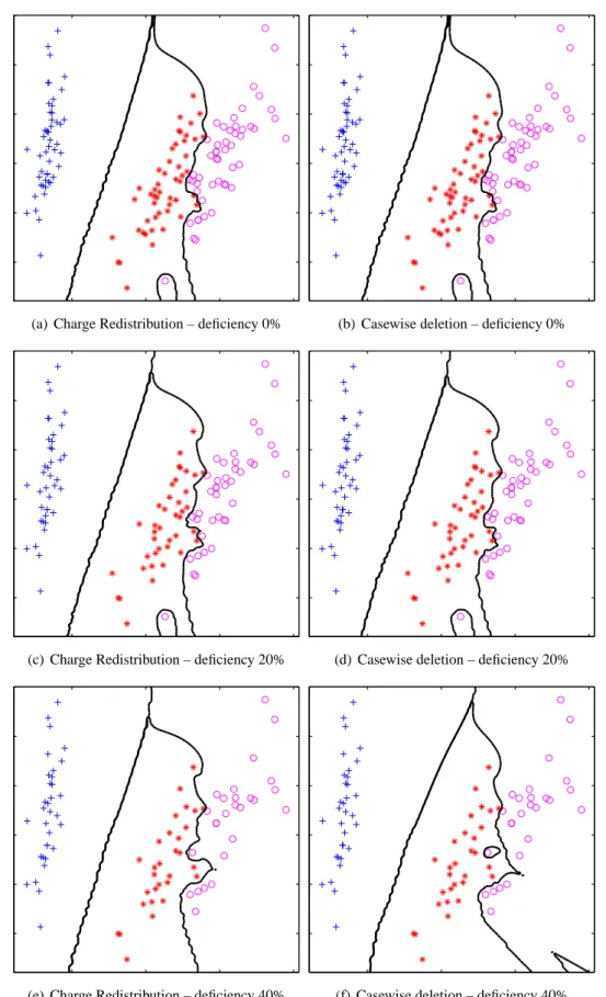
3.7 EFC decision boundaries for a 2–D PCA projection of the Iris dataset for Charge Redistribution (left column) and casewise deletion (right column) as the deficiency level increases. . . 45
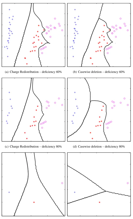
3.8 EFC decision boundaries for a 2–D PCA projection of the Iris dataset for Charge Redistribution (left column) and casewise deletion (right column) as the deficiency level increases (contd.) . . . 46
3.9 Decision boundaries for complete and maximally deficient PCA projection of the Iris dataset . . . 48
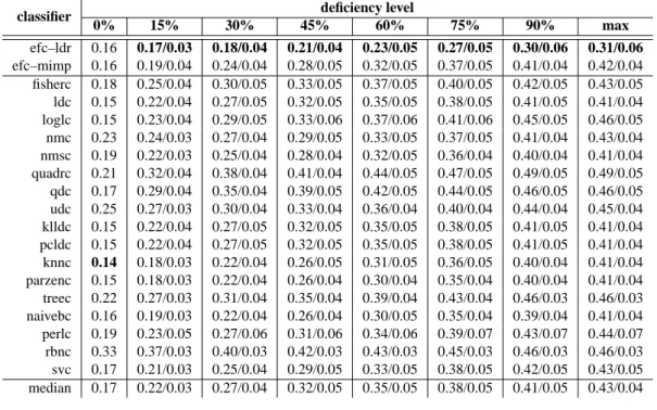
3.10 Performance for incomplete test data and various deficiency levels (recognition rates) . . 48
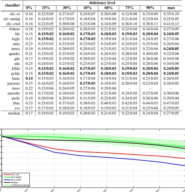
3.13 Performance for missing labels and various deficiency levels (recognition rates) . . . 52
3.14 Performance for missing labels, incomplete both test and training data and various deficiency levels (recognition rates) . . . 53
4.1 Hold–out method; ‘f1’,‘f2’,‘f3’ denote features, ‘id’ denotes instance indexes . . . 56
4.2 Cross–validation; ‘f1’,‘f2’,‘f3’ denote features, ‘id’ denotes instance indexes . . . 57
4.3 Bootstrap method; ‘f1’,‘f2’,‘f3’ denote features, ‘id’ denotes instance indexes . . . 58
4.4 Density Preserving Sampling procedure; ‘f1’,‘f2’,‘f3’ denote features, ‘id’ denotes instance indexes . . . 64
4.5 Synthetic datasets . . . 65
4.6 Cone–torus – scatter plots of 8 DPS–S folds . . . 66
4.7 Cone–torus – scatter plots of 8 CV folds . . . 66
4.8 Cone–torus – decision boundaries for qdc trained on DPS–S (solid line) and CV (dotted line) folds . . . 67
4.9 Synth–mat – decision boundaries for qdc trained on DPS–S (solid line) and CV (dotted line) folds . . . 67
4.10 Mean correntropy between each fold and the original dataset . . . 68
4.11 Mean between–fold correntropy . . . 68
4.12 Mean absolute bias (averaged over all classifiers). . . 69
4.13 Mean absolute bias (averaged over all datasets) . . . 69
4.14 Standard deviation of error estimate (averaged over all classifiers) . . . 70
4.15 Standard deviation of error estimate (averaged over all datasets) . . . 70
4.16 Bias of DPS error estimate calculated using a single fold (averaged over all classifiers) . 73 4.17 Correlation between bias and correntropy . . . 73
4.18 Single model v. combination errors for Cone–torus dataset . . . 74
4.19 Single model v. combination errors for Synth–mat dataset . . . 74
4.20 Discrete Error Distributions for Cone–torus dataset and qdc (error rates given in brackets) 74 4.21 Discrete Error Distributions for Synth–mat dataset and treec (error rates given in brackets) 75 5.1 Contour plots for the toy problems: solid line –p(x), dotted line –q(x) . . . 85
5.2 Parzen density based Kullback–Leibler divergence estimator DˆKL (horizontal axis – sample size, vertical axis – estimated value) . . . 89
5.3 kNN density based Kullback–Leibler divergence estimator D˜KL (horizontal axis – sample size, vertical axis – estimated value) . . . 90
5.4 Parzen density based Jeffrey’s divergence estimatorDˆJ (horizontal axis – sample size, vertical axis – estimated value) . . . 91
5.5 kNN density based Jeffrey’s divergence estimator D˜J (horizontal axis – sample size, vertical axis – estimated value) . . . 92
5.6 Parzen density based Jensen–Shannon’s divergence estimator DˆJS (horizontal axis – sample size, vertical axis – estimated value) . . . 93
5.7 kNN density based Jensen–Shannon’s divergence estimator D˜JS (horizontal axis – sample size, vertical axis – estimated value) . . . 94
5.8 Parzen density based ISE estimatorISEˆ (horizontal axis – sample size, vertical axis – estimated value) . . . 96
5.9 kNN density based ISE estimator ISE˜ (horizontal axis – sample size, vertical axis – estimated value) . . . 97
5.11 Correlation between bias and divergence estimates averaged over the latter . . . 100
5.12 Correlation coefficient histograms for all dataset/classifier/divergence estimator triplets . 100 5.13 Histograms of datasets and divergence estimators for the 198 constant divergence no–correlation cases (numbers of cases denoted on the vertical axis) . . . 101
5.14 Correlation between signed bias and divergence estimates, averaged over datasets . . . . 101
5.15 Correlation map for signed bias and divergence estimates, averaged over classifiers . . . 102
5.16 Correlation maps for each dataset and signed bias (axes like in Figure 5.14) . . . 103
5.17 Correlation coefficient histograms for each divergence estimator and signed bias (X axis: [−1,+1], Y axis:[0,+40]) . . . 104
5.18 Histograms of datasets, classifiers and divergence estimators for the 806 high (≥ 0.9) signed bias correlation cases (numbers of cases denoted on the vertical axis) . . . 105
5.19 Scatter plots of the Cone–torus subsamples for lowest divergence values with superimposed decision boundaries of the qdc classifier . . . 106
5.20 Scatter plots of the Cone–torus subsamples for highest divergence values with superimposed decision boundaries of the qdc classifier . . . 107
6.1 Regression error (MSE) on PCA transformed dataset v. the number of principal components115 6.2 Predicted v. target values for the blind–test data . . . 118
6.4 Statistical properties of the data . . . 122
6.5 Mean imputation (dashed vertical line) v. imputation from univariate distribution (solid vertical line) for the 10thfeature, superimposed on the PDF (blue solid line) . . . 132
6.6 Nested cross–validation scheme. NFOLD denotes the total number of folds. . . 132
6.7 Test versus validation errors (mean values of repeated cross–validation). . . 134
6.8 Test versus validation errors (mean values + stdev of repeated cross–validation) . . . 134
6.9 Misclassification rates of the best level 2 models for each test object (NCV) . . . 135
3.1 Dataset details . . . 47
3.2 Performance for incomplete test data and various deficiency levels . . . 49
3.3 Performance for incomplete training data and various deficiency levels . . . 50
3.4 Performance for incomplete both test and training data and various deficiency levels. . . 51
3.5 Performance for missing labels and various deficiency levels . . . 52
3.6 Performance for missing labels, incomplete test and training data and various deficiency levels . . . 53
4.1 Bias and variance summary . . . 70
4.2 Ranking of top 3 classifiers . . . 71
4.3 Correlation between true generalisation error and error estimates . . . 72
5.1 Divergence measure estimators . . . 87
5.2 Automatic bandwidth selection methods . . . 87
5.3 Gaussian kernel covariance matrix . . . 88
6.1 Details of toxicity prediction descriptors and training/test datasets . . . 112
6.2 Regression error on PCA transformed dataset / errors reported in the literature . . . 114
6.3 First–Pass Winners ranking / DPS–U performance . . . 117
6.4 Mussel biomarker data class details . . . 120
6.5 Experiment scenarios . . . 123
6.6 10–fold cross–validation errors . . . 123
6.7 8–fold Density Preserving Sampling errors (DPS–S) . . . 124
6.8 Leave–one–out cross–validation errors. . . 124
6.9 Classification errors after removal of a single feature (10–fold CV) . . . 127
6.10 Classification errors after removal of a single feature (8–fold DPS–S) . . . 127
6.11 Single feature classification errors (10–fold CV) . . . 128
6.12 Single feature classification errors (8–fold DPS–S) . . . 128
6.13 Classification errors for PCA–transformed dataset (10–fold CV) . . . 129
6.14 Classification errors for PCA–transformed dataset (8–fold DPS–S) . . . 129
6.15 Test errors of combinations, component and candidate classifiers (NCV) . . . 133
6.16 Test errors of combinations, component and candidate classifiers (NDPS) . . . 133
A.1 Benchmark datasets summary . . . 145
B.1 Classifiers used in the experiments. . . 151
B.2 Regressors used in the experiments . . . 153
First of all I would like to thank my supervisor Prof. Bogdan Gabrys for inspiring and encouraging me to take on this PhD project. I am also very thankful for his expert advice, invaluable feedback and most importantly, for keeping me motivated at all times. Special thanks also go to Dr. Katarzyna Musiał for quick and efficient proofreading.
The data used in Section 6.3 was collected during the ‘Developing an Index of the Quality of the Marine Environment (Marine Environment I.Q.) based on biomarkers’ project no. 173343/S40, funded by the Research council of Norway. Thanks are due to the staff at IRIS – Biomiljø for providing the data and collaboration.
Others who contributed to this work are the anonymous reviewers who gave me their valuable feedback to my academic output. Their comments and insights also helped to improve many aspects of this work.
I would also like to thank my wife Dominika for constant support and understanding. Finally, I would like to express my gratitude to my parents for always pushing me in the right direction in both personal and academic sense. This thesis is also dedicated to the memory of those who are no longer with us.
The work contained in this thesis is the result of my own investigations and has not been accepted nor concurrently submitted in candidature for any other award.
The abbreviations are given in an alphabetical order.
AMISE Asymptotic Mean Integrated Squared Error
ANN Artificial Neural Network
BSS Blind Source Separation
CIP Cross–Information Potential
CR Charge Redistribution
CV Cross–Validation
CWD Casewise Deletion
DPS Density Preserving Sampling
DPS–S Supervised DPS
DPS–U Unsupervised DPS
DPS–SU Supervised + Unsupervised DPS
LOO Leave–One–Out
EFC Electrostatic Field Classifier
EFCF Electrostatic Field Classification Framework
EM Expectation Maximisation
GFMM General Fuzzy Min–Max
GCF Generalised Correlation Function
GFC Gravity Field Classifier
GTU Generalised Theory of Uncertainty
ICA Independent Component Analysis
IF Information Force
IP Information Potential
ISE Integrated Squared Error
ITL Information Theoretic Learning
JIP Joint Information Potential
kNN k–Nearest Neighbour
LDA Linear Discriminant Analysis
LDR Local Dimensionality Reduction
MAE Mean Absolute Error
MAR Missing At Random
MCAR Missing Completely At Random
MCS Multiple Classifier System
MI Mutual Information
MIF Marginal Information Force
MIMP Mean Imputation
MIP Marginal Information Potential
MISE Mean Integrated Squared Error
ML Maximum Likelihood
MLP Multi–Layer Perceptron
MNAR Missing Not At Random
MMI Maximum Mutual Information
MRS Multiple Regressor System
MSE Mean Squared Error
MV Majority Voting
NCV Nested Cross–Validation
NDPS Nested Density Preserved Sampling
OLS Ordinary Least Squares (regression)
PC Pre–Classification
PCA Principal Component Analysis
PCs Principal Components
PDF Probability Density Function
PLS Partial Least Squares (regression)
PMIP Partial Marginal Information Potential
PV Plurality Voting
RoT Rule of Thumb method
QSAR Quantitative Structure–Activity Relationship
RBF Radial Basis Function
RMSE Root Mean Squared Error
SVM Support Vector Machine
UCIP Unnormalised Cross–Information Potential
Notation
symbol description example
x scalar value x= 1
xi scalar value asithelement of a set f(xi) = 2xi
x column vector x= 1 2 ,x= x1 x2
xi column vector asithelement of a set f(xi) = 2xi
X matrix X=
x1,1 x1,2
x2,1 x2,2
Xi vector asithcolumn of a matrix X=X1 X2 . . . XN
X[R×C] matrix withRrows andCcolumns X=
x. . .1,1 x. . .1,2 . . .. . . x. . .1,C xR,1 . . . xR,C X set X ={x1, x2, . . . , xN}
X random variable or scalar, depending on the context D={(X, T)}, N = 100
Since a part of this thesis has been devoted to sampling techniques, for consistency a convention used by statisticians has been followed and the word ‘sample’ denotes a collection of data instances rather than a single instance, which is often the case in the machine learning literature.
if we will keep our eyes and ears open.” Ralph Waldo Emerson (1860), ”Conduct of Life”
Introduction
The amount of digital data generated worldwide every year is growing at an unprecedented rate. Automatic data acquisition and storage through website tracking, loyalty programmes, industrial process monitoring or medical records to name a few, has never been so cheap and easy. According to the IBM UK predictions, the amount of digital data in the world will double every 11 hours by the end of this year [27].
It might seem that one of the major challenges we are now facing is how to utilise this massive amounts of data to its full potential. There are however other problems, the machine learning community has been trying to address for many years, which concern the quality of acquired data. Unfortunately none of the data acquisition procedures, be it automatic or manual, is perfect in practice. There are many reasons for this. The sensors we are using to monitor various processes have limited precision and sometimes fail, leading to either noisy or outlying measurements, or even no measurements at all. The chemical or biological tests we perform are often mutually exclusive and destructive, leaving us with incomplete information to support further decisions. Finally, human errors made during data collection or while later entering the data into the database also are a source of inconsistences. Moreover, we should always remember that although often used as such, in general the term ‘data’ is not a synonym of ‘information’. Thus there is always a risk that a data collection process, if not planned consciously and carefully enough, can produce a huge amount of useless numbers, resulting in waste of both time and money.
The pursuit of addressing the issues emerging from growing amounts of varying quality data, often stored in different, incompatible formats, left the smart information systems evolving into large number of very specific techniques only capable to work in highly constrained environment, on limited evidence and with poor complexity control mechanisms. This induces the need for some kind of unifying framework, an information–based ‘theory of everything’ [45] many researchers are constantly looking for.
1.1
Background
With a magnitude of various, constantly evolving predictive modelling techniques in use, the number of completely novel approaches designed from scratch is relatively low. By looking at the last 30 years or so, there was only a handful of truly seminal, ground–breaking inventions in the machine learning field, some dating back even to the mid 20thcentury.
In the very early days of machine learning, when the computational power was very expensive and in general not easily accessible, the rule based expert systems, sometimes referred to as the1st generation methods, were a dominating approach [33]. They didn’t have high computational
demands, yet in many applications they have performed sufficiently well. A common feature of all rule based systems is, that the decision making process is completely transparent, so it is always possible to explain exactly why the final decision is what it is. This fact in conjunction with reasonable performance in some applications results in expert systems still being used today in a number of cases, like banking or finance planning [79]. Perhaps the biggest drawback of rule based systems is that the rules had to be created manually by a knowledge engineer on the basis of knowledge extracted from domain experts. The knowledge extraction was a daunting process not only because the experts often did not agree with each other, but also because their predictions in many cases tended to be inaccurate. Moreover as the system evolved, the number of rules had to grow, as was the case with the number of exceptions to the rules and then exceptions to exceptions etc. The systems thus started losing their simplicity and transparency. Clearly, some new workhorse of machine learning was needed.
The increase in computational power and its accessibility enabled researchers to look in another direction – learning directly from data and not from the experts anymore. Due to the increasing number of success stories of the Artificial Neural Networks (ANNs) in various applications [11, 69] a huge paradigm shift towards learning from exemplars has been observed, with a central belief that all information needed to develop a predictive model is contained in the data. Domain knowledge has started to be seen as unnecessary, partly because it wasn’t easily integrable into the ANN models. The shift to the learning from exemplars paradigm has brought a group of new, previously not known problems, like estimation of the generalisation ability of the developed model [181], the multitude of local minima encountered during model training, which is usually a gradient–driven optimisation process and many more. Nevertheless, the late 80s and the 90s were definitely dominated by the neural networks.
At the beginning of the 21st century the interest has gradually switched towards a new technique – the Vapnik’s Support Vector Machines (SVMs) [28, 176, 177], which do not have many of the drawbacks of neural networks and have very sound theoretical foundations. The large number of past and current success stories (the three publications on SVMs referenced above currently have in excess of 45k citations), makes SVMs the state–of–the art technique for classification and regression as of today. SVMs, as well as neural networks are sometimes regarded as the2ndgeneration machine learning methods.
Throughout the years there was also a great deal of research effort focused on the application of probability theory to machine learning. The Bayesian artificial intelligence and especially Bayes networks designed and used with the help of graphical models are more and more often seen as the technique for bridging the gap between the domain knowledge driven and data–driven approaches [12, 93]. Although the Bayesian framework effortlessly combines them both, and is especially well suited for online learning, as always, there are some problems. One of the most important is the computational complexity of calculations involving manipulation of possibly high–dimensional probability density functions (PDFs). Since in all but the simplest cases this cannot be done exactly, a number of approximate methods like variational Bayes [12] or expectation propagation [109] has been designed to address this issue. This raises an important question of how much and in what circumstances one can trust the estimates. The reality is that often for the estimates of the probability density functions to be at least remotely accurate, one needs immense amounts of data, which are very computationally costly to process. Nevertheless, the probabilistic Bayesian models certainly have the potential of becoming the 3rd generation machine learning techniques.
All the methods briefly discussed above differ at various levels. One of these differences is the inspiration underlying their development by pushing researchers in previously unexplored
directions. The natural environment is without a doubt the most fruitful source of inspiration in the field of machine learning. At a very high level, observation of a decision making processes performed by the human experts resulted in the development of expert systems. At a lower level, an attempt to copy the principles of operation of human brain led to invention of the ANNs. The multiagent systems [39] or Genetic Algorithms (GA) [51] are just a few more examples.
The mathematical and statistical theories are another rich sources of inspiration, leading to development of the already mentioned Support Vector Machines and the whole field referred to as the Bayesian Artificial Intelligence.
There is however another, often overlooked source of potential inspiration – physics. There exist tremendous similarities between physical world and artificial intelligence in the context of machine learning. At the elementary level of information, uncertainty and complexity matter and information naturally intertwine with each other and the physics of matter and energy often provides the best description of information and its uncertainty [186]. In this setting energy defined as an ability to do work corresponds to uncertainty as an ability to obtain information.
The inherent self–organisation property of various physical systems, which leads to complex emergent behaviour of interacting parts, resulting from following a small set of elementary rules [7] is yet another interesting phenomenon. This property at an individual particle level not only strongly resembles machine learning tasks like clustering or data transformation, but also perfectly fits within the ‘learning from exemplars’ paradigm mentioned earlier.
Finally, with numerous machine learning problems which still remain open, the guidance of well established and understood physical models may prove extremely beneficial.
1.2
Project description and goals
The main objective of this research project is to explore and investigate some of the similarities between physical world and computational intelligence in order to find inspirations and design a new breed of nature inspired machine learning techniques. The rationale behind this line of research lies in an attempt to adopt the well defined and formalised knowledge describing the physical world to the immature artificial learning field.
This research intends to bridge the gaps between physics and machine learning and provide more efficient and intelligent means for fuller exploitation of evidence which is available with varying quality and in varying quantities. Inspirations for the artificial learning modelling were exploited by a direct application of physical principles describing potential fields to multivariate data vectors treated as charged particles, as well as by using the recently developed Information Theoretic Learning (ITL) framework for online estimation and manipulation of entropy, which also demonstrates deep analogies with physical fields, but without being so strictly constrained.
The study presented in this thesis explores and targets various challenging aspects of the classical predictive system development cycle. This is achieved by exploring usability of strong physical analogies as well as weaker physical inspirations for providing alternative to existing solutions and proposing completely novel ones.
The goals of this research project can be summarised as:
1. To develop and validate on real problems, a predictive system design methodology which would facilitate building of well–performing predictive models, even in the absence of domain knowledge. Application of this purely data–driven methodology to real–world problems should result in predictive systems with performance comparable to the ones designed by the experts in a given problem domain. This will be achieved by offsetting
the lack of domain knowledge by additional computations and automation of all possible activities, which are usually performed manually.
2. To develop a unified classification framework by exploiting the concept of dynamic data–particle based optimisation processes and physical fields interaction, with inherent support for handling deficient inputs and ability to learn not only from labelled data, but also from a mixture of both labelled and unlabelled datasets.
3. To facilitate efficient learning from large datasets, where the computational requirements are currently the biggest obstacle, by addressing this issue at the high level, independent of the actual machine learning model used, taking advantage of the ITL criteria.
The above goals address the predictive system design process at different levels, from individual base models to validation of obtained systems to proposing a novel generalised methodology for building multistage predictive models. As such, they can also be seen as a proof of concept, confirming the potential of physically inspired methods in the field of machine learning.
1.3
Original contributions and publications resulting from this work
The original contributions of this work are:• Derivation of a rigorous predictive system development methodology/cycle, verified on two real–world problems including the Environmental Toxicity Prediction Challenge CADASTER 2009 [17]. The developed purely data–driven predictive system was awarded as the First–Pass winner, non–significantly different from the top performing submission. • Comprehensive, extendible Electrostatic Field Classification Framework (EFCF) for
supervised and semi–supervised learning from incomplete data [15, 20], which takes advantage of a direct analogy with physical fields by treating multivariate data vectors as charged, interacting particles.
• Novel Density Preserving Sampling (DPS) technique [16, 18] as an alternative to standard, commonly used cross–validation (CV), reducing the computational requirements of generalisation error estimation procedure by an order of magnitude, without compromising the quality of estimate and protecting against typical pitfalls connected with random sampling. DPS is a result of indirect physical inspiration in a form of Information Theoretic Learning framework for online entropy estimation and manipulation.
• Experimental comparative study of probability density function divergence estimators and their usability in sampling for generalisation error estimation [19]. The study calls into question the accuracy of the estimators for datasets smaller than thousands of instances. Nevertheless an attempt is made to exploit the divergence estimators for representative sampling to further reduce the computational requirements of generalisation error estimation by another order of magnitude when compared to 10 times repeated 10–fold cross–validation.
• Multi–stage Multiple Classifier System (MCS) for robust predictive modelling of water pollution using biomarker data [21, 119], developed by taking advantage of the proposed predictive system development methodology and a Missing Not at Random (MNAR) data modelling approach.
The following peer–reviewed conference and journal publications are a result of this work: • M. Budka and B. Gabrys, “Electrostatic Field Classifier for Deficient Data”, in Computer
Recognition Systems 3, ser. Advances in Soft Computing, M. Kurzynski and M. Wozniak,
Eds. Springer, 2009, vol. 57, pp. 311–318.
• M. Budka and B. Gabrys, “Electrostatic field framework for supervised and semi–supervised learning from incomplete data”, Natural Computing,
DOI:10.1007/s11047-010-9182-4.
• M. Budka, B. Gabrys, and E. Ravagnan, “Robust predictive modelling of water pollution using biomarker data”, Water Research, vol. 44, no. 10, pp. 3294–3308, 2010.
• M. Budka and B. Gabrys, “Ridge regression ensemble for toxicity prediction”, Procedia
Computer Science, vol. 1, no. 1, pp. 193–201, 2010.
• M. Budka and B. Gabrys, “Correntropy–based density–preserving data sampling as an alternative to standard cross–validation”, in Proceedings of the IEEE World Congress on
Computational Intelligence. IEEE, 2010, pp. 1437–1444.
• M. Budka and B. Gabrys, “Density Preserving Sampling (DPS) for error estimation and model selection”, IEEE Transactions on Pattern Analysis and Machine Intelligence, 2010 (Submitted).
• M. Budka and B. Gabrys, “On accuracy of PDF divergence estimators and their applicability to representative data sampling”, IEEE Transactions on Knowledge and Data
Engineering, 2010 (Submitted).
• D. Pampanin, E. Ravagnan, S. Apeland, N. Aarab, B. Godal, S. Westerlund, D. Hjermann, T. Eftestøl, M. Budka, B. Gabrys, A. Viarengo, and J. Barsiene, “The Marine Environment I.Q. concept. Developing an Index of the Quality of the Marine Environment based on biomarkers: integration of pollutant effects on marine organisms.” in Proceedings of
the 27th ESCPB (New European Society for Comparative Physiology and Biochemistry) Congress, 2010 (Accepted).
1.4
Organisation of the thesis
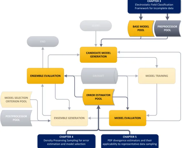
The structure of this thesis and the dependencies between the chapters have been outlined in Figure 1.1. Chapter 2 provides a high level introduction to machine learning and physically inspired techniques. The first part of the chapter focuses on the predictive system development cycle, describing its classical form and then proposing a generalised version of the cycle for data–driven design of predictive systems. In the course of the proposed cycle description, necessary machine learning concepts are progressively introduced whenever a need arises. This way the whole description follows a logical sequence rather than frequently referencing the reader to a dictionary of used terms. The second part of the chapter includes a description of a number of selected physically inspired artificial learning techniques developed to date, and forms the theoretical basis for the rest of this thesis.
In Chapter 3 the first development resulting from this work, in a form of a comprehensive Electrostatic Field Classification Framework is described. An original approach to exploiting incomplete training data with missing features, involving extensive use of electrostatic charge analogy, has been used. The framework supports a hybrid supervised and unsupervised training
Figure 1.1:Structure of the thesis and chapter dependencies
scenario, enabling learning simultaneously from both labelled and unlabelled data using the same set of rules and adaptation mechanisms. Classification of incomplete patterns has been facilitated by introducing a Local Dimensionality Reduction (LDR) technique, which aims at exploiting all available information using the data ‘as is’, rather than trying to estimate the missing values. The performance of all proposed methods has been extensively tested in a wide range of missing data scenarios, using a number of standard benchmark datasets in order to make the results comparable with those available in current and future literature. Several modifications to the original Electrostatic Field Classifier (EFC) aiming at improving speed and robustness in higher dimensional spaces have also been introduced and discussed.
Chapter 4 has been devoted to the ITL–based Density Preserving Sampling technique as an alternative to the standard cross–validation, which unlike the latter is not stochastic and thus does not require multiple repetitions in order to produce reliable results, leading to considerable computational savings. DPS divides the available data into subsets by maximising a measure of representativeness of the input dataset. This allows to produce low variance error estimates with accuracy comparable to 10 times repeated cross–validation at a fraction of computations required by CV. The method can also be successfully used for model ranking and selection. The usability and performance of DPS is investigated using a set of publicly available benchmark datasets and standard classifiers.
In Chapter 5 the possibility of selecting a representative subset of data from a larger dataset in a context of accurate estimation of the generalisation performance of a predictive model is further investigated. An experimental comparative study of various estimates of a range of probability density function divergence measures, using a number of synthetic and benchmark datasets is performed. While correlation of the generalisation error with divergence was the primary motivation of this study, it has led to more fundamental analysis of usefulness of the divergence measures, and more accurately their estimators.
Chapter 6 has been devoted to the application of the proposed generalised predictive system development cycle and physically inspired methods to two real–world environmental problems: toxicity prediction and marine pollution monitoring. It is demonstrated that purely data–driven approaches can successfully compete with predictive models developed by the experts in their respective areas. The impact of the physically inspired models derived in this thesis on the two problems is also investigated.
The concluding Chapter 7 summarises the main findings of the project and indicates directions for further research.
Machine learning and physically
inspired techniques
2.1
Introduction
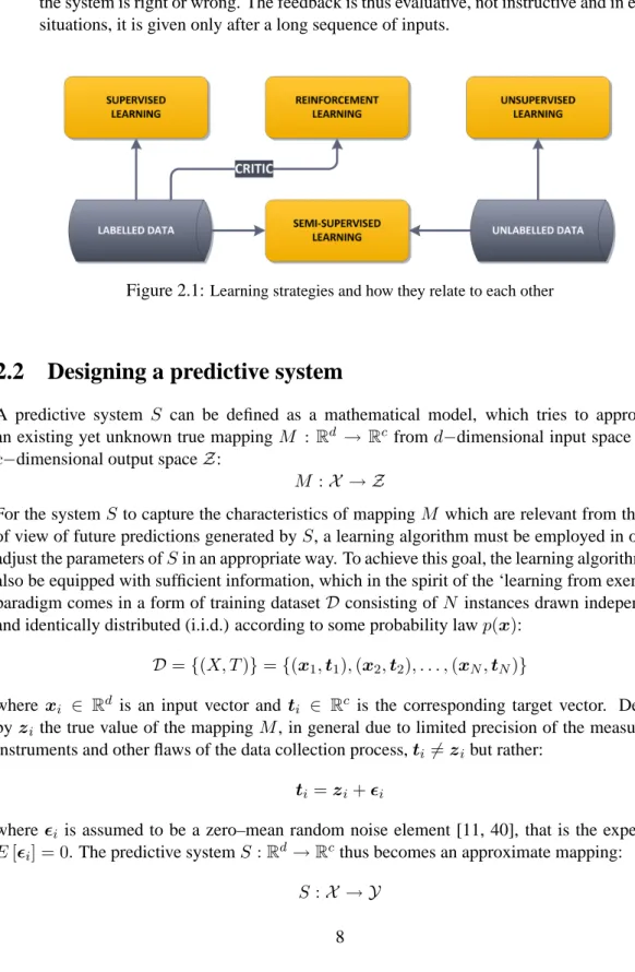
There are many different definitions of machine learning in the literature [4, 12, 40, 110, 162]. At the lowest level of abstraction learning can be described as estimation of the parameter values of a learning machine using a set of available exemplars in order to optimise some criterion function [40]. This definition not only covers all learning scenarios presented in Figure 2.1, but at the same time, in the spirit of the ‘learning from exemplars’ paradigm, also emphasises the role of training data used during parameter estimation. There are however other ways of looking at the process of machine learning. One of the most general definitions assumes that the learning machine is exposed to a single or multiple sources of information and the goal of learning is to explore and exploit the redundancies from these sources [128].
Whichever definition one chooses to adopt, any method that incorporates information from training data necessarily implies some form of learning. Based on the availability and type of data, the following forms of learning, also presented in Figure 2.1, can be distinguished [40]:
• Supervised learning also known as learning with a teacher, in which the learning machine
is provided not only with the input data, but also with the corresponding values of the target variable. An example can be a classification task, in which the predictive system is expected to learn how to recognise handwritten characters, and is given both the input data (e.g. a bitmap representing the character) as well as the class label (e.g. information which character the bitmap actually represents). Another example of supervised learning is regression, in which the model learns how to predict values of a continuous (rather than discrete) variable on the basis of available input data.
• Unsupervised learning also known as learning without a teacher, in which the learning
machine is provided with the input data only. This kind of learning is usually associated with data density estimation or clustering, in which a natural grouping of the input instances is sought. The word ‘natural’ implies grouping the instances in such a way, that the ones belonging to the same group are similar to each other but dissimilar to the rest. The result of clustering thus strongly depends on the adopted definition of the similarity measure.
• Semi–supervised learning, which is a mixture of both supervised and unsupervised
for supervised learning is limited for various reasons, unlabelled data is abundant and easy to obtain. Semi–supervised learning algorithms try to take advantage of this fact in order to improve their predictive power and accuracy.
• Reinforcement learning also known as learning with a critic, which is an intermediate
learning strategy between supervised and unsupervised learning. In reinforcement learning the only information available, apart from the input variables, is if the prediction of the system is right or wrong. The feedback is thus evaluative, not instructive and in extreme situations, it is given only after a long sequence of inputs.
Figure 2.1:Learning strategies and how they relate to each other
2.2
Designing a predictive system
A predictive system S can be defined as a mathematical model, which tries to approximate an existing yet unknown true mappingM : Rd → Rc fromd−dimensional input spaceX into
c−dimensional output spaceZ:
M :X → Z (2.1)
For the systemS to capture the characteristics of mappingM which are relevant from the point of view of future predictions generated byS, a learning algorithm must be employed in order to adjust the parameters ofSin an appropriate way. To achieve this goal, the learning algorithm must also be equipped with sufficient information, which in the spirit of the ‘learning from exemplars’ paradigm comes in a form of training datasetDconsisting ofN instances drawn independently and identically distributed (i.i.d.) according to some probability lawp(x):
D={(X, T)}={(x1,t1),(x2,t2), . . . ,(xN,tN)} (2.2)
where xi ∈ Rd is an input vector and ti ∈ Rc is the corresponding target vector. Denoting
by zi the true value of the mapping M, in general due to limited precision of the measurement
instruments and other flaws of the data collection process,ti 6=zibut rather:
ti =zi+i (2.3)
where i is assumed to be a zero–mean random noise element [11, 40], that is the expectation
E[i] = 0. The predictive systemS :Rd→Rc thus becomes an approximate mapping:
where Y is the space of predictions generated by S. It is interesting to note that the above definition applies to both regression and classification problems, as they differ only by the possible values the target variable can take (continuous or discrete).
In order to measure how well a predictive system models the unknown mapping, an error function is used, which in a general form can be written as:
err(Y, T) = 1 N N X i f(yi,ti) (2.5)
where for regression problems typically f(a, b) = (a−b)2 leading to the Mean Squared Error
(MSE) function [11, 40] discussed in more detail in the following sections. In the case of classification problems with the target variable being a discrete scalar value representing the class label, oftenf(a, b) = (1−δa,b), whereδa,bis the Kronecker delta function given by:
δa,b=
(
1, ifa=b
0, ifa6=b (2.6)
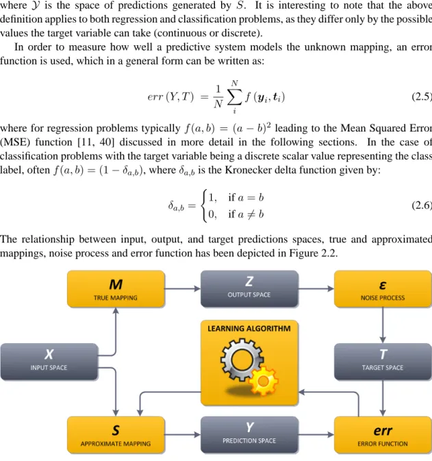
The relationship between input, output, and target predictions spaces, true and approximated mappings, noise process and error function has been depicted in Figure 2.2.
Figure 2.2: Relationship between input, output, and target predictions spaces, true and approximated mappings, noise process and error function
2.2.1 Classical predictive system design cycle
In order to build a well–performing predictive model a systematic approach should be taken, usually leading to an iterative design procedure. A classical predictive system design cycle has been depicted in Figure 2.3 [40]. The cycle entails a number of clearly defined steps, which must be followed and repeated if needed, until a satisfactory result is obtained.
Data collection
The procedure which can account for a large part of time and cost required to develop a system. The main problem at this stage is how to tell that the amount of collected data is sufficient and
Figure 2.3:Classical design cycle of a predictive model
that the data is representative. In the considerations contained in this thesis it is usually assumed that the data has already been collected and the data acquisition process itself is not investigated, with one exception of the biomarker data used in the study described in Chapter 6.
Feature selection
A critical step strongly depending on the problem, often making use of available prior/domain knowledge, but also possible to be performed in a purely data–driven way. This step involves selection and/or transformation of features/attributes which have been measured during data collection. The selected features should be relevant, simple to extract, insensitive to noise and to irrelevant transformations but it may turn out, that due to a flawed data acquisition procedure none of the features is of any use. The problems which arise here, apart from the obvious ‘how to select good feature subset’ are often much more subtle, like how not to select wrong features, how to combine domain knowledge with empirical evidence or how many features to choose.
Model selection
With a magnitude of different predictive models to choose from, ranging from simple linear classifiers and regressors, to Artificial Neural Networks and Support Vector Machines, how to choose a correct one for the problem at hand? Or better yet, how to tell if the current model is good or not? One possible solution used throughout this thesis is to select multiple diverse models rather than a single one and combine them to obtain a Multiple Classifier/Regressor System (MCS/MRS) also known as the ensemble model. The problem of scoring the models and discarding the ones which are useless however still remains. Also, if prior knowledge e.g. on suitability of some class of models for similar problems is available it can be used here, but one should not depend on the domain knowledge entirely.
Model training
Training is the process of adjusting model parameters to fit the data. There are many different procedures for training even the same class of models, e.g. the Artificial Neural Networks. For practical considerations, two ANNs trained using different methods are usually treated as two separate models, which shifts the problem of choosing a learning procedure towards model selection. The choice of data for training is also not a trivial issue – should all available data be used to train a model or only some part of it? If only a part of data is to be used, how large should it be, and more importantly, how should it be selected?
Model evaluation
A critical step involving assessment of performance of the designed system and identification of components which need improvements. The central difficulty is what measure of performance to use and how to estimate it. For example, should the error on the training data be used for model evaluation? Or maybe an error on novel, previously unseed data would be a better choice? And if one decides to use the latter, where to get more data? Or perhaps it is possible to do without it?
At this step it is possible to repeat any number of previous steps if model evaluation reveals unsatisfactory performance. In theory thus, the design cycle could be repeated many times, for example using random subsets of features or randomly selected models. In practice however the available computational resources are usually the limiting factor. Does it mean that one should give up randomness completely, although it is known to be useful in many practical cases [11, 40]? Or maybe there is a controlled way to take advantage of the benefits of randomness without stretching the computational resources too much? In order to answer all these questions, a more advanced predictive system methodology is needed.
2.2.2 Generalised predictive system design cycle
A generalised predictive system design cycle, which has been followed in order to develop successful systems described in Chapter 6, is proposed below. Similarly to the classical cycle, it is a number of clearly defined steps one needs to follow to develop a reasonably performing predictive system. The generalised cycle has been depicted in Figure 2.4. The main assumption is that the data has already been acquired, so the data collection step can be omitted. Before describing the proposed design cycle, some of the terms used in Figure 2.4 and the description itself are explained below:
• Base model pool is a set of classification or regression models, depending on the problem.
For the list of base models used in this thesis please refer to Tables B.1 and B.2.
• Preprocessor pool is a set of data preprocessing methods, including but not limited to:
– feature selection algorithms (e.g. greedy methods – forward, backward,
plus–L–takeaway–R [40, 175], semi–random methods – Genetic Algorithms [8, 51] or Simulated Annealing [24, 90] and random methods),
– linear and non–linear feature transformation (e.g. Principal Component Analysis
(PCA) [87], Linear Discriminant Analysis (LDA) [48], Maximum Mutual Information (MMI) projection [9, 166, 167, 168, 169, 170, 165]); some of these methods are discussed in more detail in Chapter 6,
– outlier detection, denoising and other data cleansing algorithms [178],
– missing data handling algorithms [63, 117, 136] if required (see Chapter 3 for a more
detailed treatment of the missing data problem and a description of some standard protocols for dealing with it).
Note that preprocessing can have multiple stages, e.g. outlier detection and removal, followed by missing data imputation, followed by Principal Component Analysis. For clarity, in Figure 2.4 and the following description of the generalised design cycle, all these steps would be denoted as a single preprocessing routine.
• Candidate model is a base model paired with one or more preprocessing technique,
e.g. an Artificial Neural Network using a subset of features (receptive field). In consecutive iterations of the main cycle, whole ensembles from previous iterations can act as candidate models, leading to multistage structures [142].
• Error estimator pool is a set of error estimation algorithms, including the hold–out and
random subsampling methods [181], the bootstrap method [44], cross–validation [29] and the Density Preserving Sampling technique proposed in Chapter 4.
• Model selection criterion pool is a set of criteria for model selection, e.g. select top N
models, select models with performance better than average, discard worst 20% of models (also known as trimming) etc.
• Postprocessor pool is a set of model combination methods used for ensemble building,
including voting combiners (e.g. Majority Voting (MV), Plurality Voting (PV)), averaging combiners (mean, median), weighted versions of the above or even any subset of base models trained on the outputs of ensemble members [139, 173].
The rationale behind using multiple base models, error estimators, pre– and postprocessing techniques is to encourage diversity in the members of the final combined model, as it is believed to have positive stabilising influence on its performance [138]. As a result, a general rule which applies to all the pools listed above is that the larger and more diverse they are, the better. However, in constructing the pools any available domain knowledge should be taken into account, e.g. which base models or preprocessing techniques are better or worse suited for a given problem.
Inspection of the data
Inspection of the data is an important activity, which should be treated as a preparatory stage before commencing with building a predictive system. Even superficial manual examination of the data using basic statistical and plotting techniques will quickly reveal any missing or outlying observations, at the same time suggesting what the potential difficulties resulting from the amount, dimensionality and quality of data can be. Inspection of data will often also suggest for example which techniques not to include in the base model or preprocessor pools (if no data is missing there is no reason to have missing data handling routines in the pool). Although the idea behind the generalised predictive model design procedure is that it can be run autonomously, the findings of this type can save a lot of computations, thus the time spent on data inspection will most likely pay back. Nevertheless due to its manual nature, the step can be treated as optional and has not been explicitly shown on the diagram in Figure 2.4. An example of biomarker data examination using standard statistical techniques is given in Section 6.3.2.
Candidate model generation
In the first step of the generalised predictive system design cycle a given number of candidate models is generated, using various preprocessing techniques and base models. Denoting the chosen base model byMB and theithchosen preprocessing technique byPpre(i), a candidate
modelMC becomes: MC = MB, Ppre(1), . . . Ppre(n) (2.7) where a single base model can be paired with multiple preprocessing methods to allow for multistage preprocessing as discussed earlier. Generation of candidate models can be achieved by combining preprocessors and base models randomly, using some form of domain knowledge or information gathered during model and ensemble evaluation in consecutive iterations of the main cycle. Even if this kind of information is used, it is important to still allow for some randomness to alleviate the danger of being caught in a locally optimal state, e.g. by using Genetic Optimisation. The goal of preprocessing is to prepare the data for further use. Apart from addressing the missing data or the outlier problems this way, the usual reason for preprocessing is the dimensionality reduction [11, 12, 40]. The potential problems resulting from working in high–dimensional spaces are collectively known as the ‘curse of dimensionality’ [11, 40]. Although this phenomenon can have many facets, they all have a common cause – the amount of data, which never seems to be enough and often covers only a fraction of the input space. This is caused by the fact, that the amount of data required to fill the input space grows exponentially with its dimensionality. The solution is to reduce this dimensionality somehow, either by selecting a subset of interesting attributes or performing a transformation into lower dimensions. The dimensionality reduction techniques are also useful from another point of view – they enable detection and removal of collinear and other irrelevant attributes, which might cause numerical problems for some base models. A more detailed treatment of some practical problems resulting from the ‘curse of dimensionality’ can be found in Chapter 6.
Model training
After the candidate models have been generated they can be trained using available training data. The problem here is that large amount of data with specified values of the target variable is usually difficult and expensive to obtain. Moreover, although it might be tempting to use all available data
for training, this would imply assessing the performance of the obtained predictor on the basis of training error only, in most cases leading to overfitting [11, 40].
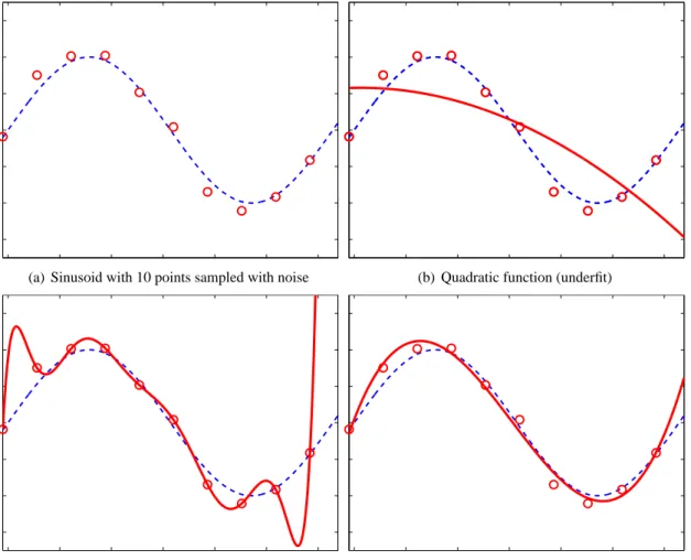
(a) Sinusoid with 10 points sampled with noise (b) Quadratic function (underfit)
(c) Degree 9 polynomial (overfit) (d) Cubic function (proper fit) Figure 2.5:Curve fitting example
In order to explain the overfitting issue, following [11] Figure 2.5 presents a simple curve fitting example. The task is to model the unknown underlying function (which is a sine) by using ten points, sampled i.i.d. with noise. This has been depicted in Figure 2.5(a), where it can be seen that most of the points do not lie exactly on the sinusoid, although they follow it closely1.
In Figure 2.5(b) a quadratic function has been fit to the data and as it can be seen, it does not capture the underlying function nor the training data – high training error would however reveal this fact. The quadratic polynomial is not complex or powerful enough to model the sinusoid and it underfits the data.
In Figure 2.5(c) a degree 9 polynomial fit to the same set of points is presented, capturing the training data perfectly. The underlaying sine function is however not captured very well, especially at the right part of the plot, where the two curves diverge. Unfortunately, since the polynomial passes exactly through all ten training points, the training error is 0, giving a false sense of a success. It is said that the model overfits the data because it is too complex for this particular problem.
1
There might be various reasons for the measurements to be noisy, usually connected with limited precision of the measurement instrument or process, thus in practice it is reasonable to assume that the data is always noisy.
The best solution appears to be a cubic polynomial, which is neither too complex nor too simple. By examining Figure 2.5(d) it can be seen that the training error is at a reasonably low level (although not 0) and the underlying function is also modelled well (although not perfectly, due to noisy input data). The problem is, that if one was to judge the model basing on the training error only, the complex degree 9 polynomial would be selected, which obviously is a suboptimal choice.
Model evaluation
The performance of all trained models is assessed at this step using one or more error estimation methods drawn from the error estimator pool. The need for using special error estimation techniques (which should not be confused with the error function given in Eq. 2.5) stems from the behaviour of the predictive models presented in Figure 2.5 and their susceptibility to overfitting. As mentioned before, the training error is usually not a good measure of future performance and the solution is to measure the error using independent test data instead [40].
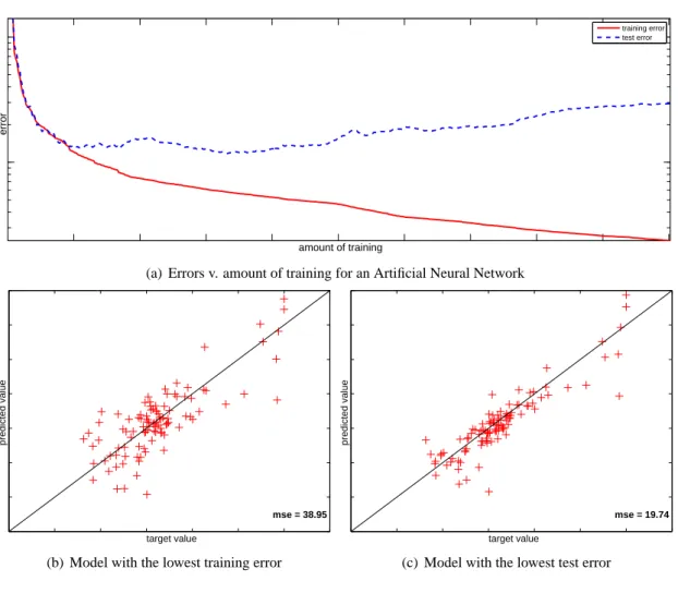
In Figure 2.6(a) the plot of training and test errors as functions of the amount of training (number of epochs – presentations of the data) for an Artificial Neural Network has been given. For presentation purposes the vertical axis has a logarithmic scale but the actual values on the axes are irrelevant for now. As the number of epochs grows, the training error (solid red curve) becomes smaller and smaller. If the network is powerful enough (that is, if it has enough adjustable parameters), due to its universal approximation property [11] the training error would eventually approach 0. The test error (dashed blue curve in Figure 2.6(a)) however behaves in a completely different way. After initial decrease, it starts climbing and the two curves move apart as the training progresses. This is a clear sign of overfitting – the network begins to ‘memorise’ the dataset, losing its generalisation ability. It is interesting to note, that for models which are not universal approximators, a plot of errors v. model complexity (degree of the polynomial in the curve fitting example of Figure 2.5) would have a similar shape.
The prediction errors of a network trained until the training error approaches 0 have been shown in Figure 2.6(b). Figure 2.6(c) presents the prediction errors of a network with minimum test error. Both plots have been created using a third, independent dataset. It’s easy to see that in case of the second network the points are much more concentred about thex=y line, which denotes better performance (for 0 error all points would lie exactly on thex=yline).
Since additional data for testing is often difficult to get hold of, a common practice is to reserve some part of available data to serve exactly this goal. The question now is, how to divide the data into a training and test part and how big should these parts be, not to risk ending up with training or test data which does not cover large parts of the input space. There exists a number of standard techniques to address this problem, which have already been mentioned in the description of the error estimator pool. A more detailed treatment of the error estimation issue can be found in Chapter 4 of this thesis.
Another important issue which needs to be discussed here is the choice of error function. Traditionally the Mean Squared Error is the most popular choice as it has been a workhorse of machine learning for many years [11]. This is due to its nice analytical properties like continuity, differentiability, existence of a number of effective optimisation algorithms or the so called bias–variance decomposition [57]. MSE however also received some criticism, mainly for not taking advantage of higher order moments of the PDF estimated from data and some ITL based alternatives have been proposed [46, 47, 103, 127, 148]. Using the notation introduced in Eq. 2.5, the Mean Squared Error function can be written as:
error
amount of training
training error test error
(a) Errors v. amount of training for an Artificial Neural Network
mse = 38.95 target value
predicted value
(b) Model with the lowest training error
mse = 19.74 target value
predicted value
(c) Model with the lowest test error
Figure 2.6: Errors as a function of the amount of training (a) and performance of models chosen on the basis of (b) training error and (c) test error
M SE(Y, T) = 1 N N X i (yi−ti)2 (2.8)
Since a single value of MSE is dependant on a given realisation of the datasetD, it is interesting to analyse the expectation of MSE considering an average over an infinite number of datasets of sizeN [11]: ED[M SE(Y, T)] = 1 N N X i EDh(yi−ti)2 i (2.9) After some manipulation and rearranging the expectation inside the sum becomes:
EDh(yi−ti)2 i = (|zi−E{zD[yi])}2 (bias)2 +EDh(yi−ED[yi])2i | {z } variance +ED2i | {z } noise (2.10)
As it can be seen, the generalisation error of a predictive system can be split into the following three components:
mappingM over all datasets of a given size. IfS was a constant function independent of the dataset, although the variance term would vanish, the bias term would most likely be very high, as the data was effectively ignored. This would result in too large values for some datasets and too small for others. In the curve fitting example presented in Figure 2.5, the model based on the quadratic polynomial is highly biased (does not fit the data very well) but has a low variance at the same time.
• Variance term, reflecting the sensitivity of the mapping S to a particular realisation of
the dataset. If S was a function which fits the training data perfectly (e.g. degree 9 polynomial of Figure 2.5(c)), the bias term would vanish (provided there is no noise) but the variance would likely be high.
• Noise term, denoting the inherent noise in the data and at the same time setting a lower
bound on the error that can be achieved.
In practice a compromise is sought to provide a good trade–off between fitting the training data and obtaining a smooth mapping able to generalise well, resulting in the so called bias–variance dilemma.
Much of what has been discussed above also applies to the classification problems. Although the error function is usually different (ANNs for classification also often use MSE). The goal is to find a smooth discriminative function, which is not too sensitive to a given realisation of the datasetDand can thus generalise well.
As mentioned before, in general the difference between the regression and classification problems lies in the type of the target variable. The implications of this fact are however quite important. While in regression the goal is to predict a value of a continuous target variable, in classification the class labels are of interest [40]. As a result, in ac−class classification problem the target variable is either a discrete scalar value between1andc, denoting membership in one of thecclasses{ω1, ω2, . . . , ωc}or ac−dimensional binary vector:
ti=ωj ⇔ ti=0 . . . 0 1 0 . . . 0T (2.11)
where the ‘1’ has been placed in thejthrow of ti. This is for example the case for ANNs with
MSE used as an objective function or any other classifier, which produces soft outputs denoting the degree of membership in each class.
The basic error function used in classification is: errclasf(Y, T) = 1 N N X i 1−δyi,ti (2.12)
which simply calculates the percentage of misclassified instances. A more elaborate approach also employs a cost function (or cost matrix) stating how expensive each type of an incorrect decision is [40]. For example, in medical diagnostics it would be much more risky and potentially dangerous to classify a person having some serious disease as healthy, than telling a healthy patient that he or she should take some additional tests because something does not seem entirely right. A very simple and often used variant of the cost function is an error weighting scheme based on class prior probabilities [42], which effectively tries to approximate the probability of error. Denoting byP(ωj)the prior probability of observing an instance belonging to thejthclass,
the probability of error becomes: perr(Y, T) = 1 N N X i P(ωti) 1−δyi,ti (2.13)
If a classifier produces a soft, probabilistic output, that is:
yi= [p(ω1|S,xi), p(ω2|S,xi), . . . , p(ωc|S,xi)]T (2.14)
and denoting byωT the true class ofxi and by ωS the class with the highest support given by
the classifier, the classification error can be decomposed as [138, 156]:
errclasf(xi) = p(ωS|S,xi) [p(ωT|xi)−p(ωS|xi)] | {z } bias + X ω6=ωS p(ω|S,xi) [p(ωT|xi)−p(ω|xi)] | {z } spread (2.15) + (1−p(ωT|xi)) | {z } Bayes error
Similarly to Eq. 2.10, the bias term represents the match of the predictive model to the classification problem, while the spread term (which is a counterpart of variance) denotes the variability of model outputs from one dataset to another. Figure 2.7(a) presents the decision boundaries of a simple, low variance linear classifier (fisherc, for details on the classifier please refer to Table B.1) superimposed on a scatter plot of a synthetic, 3–class Cone–torus dataset (Table A.1).
(a) High bias/low variance linear classifier (b) Low bias/high variance Nearest Neighbour classifier Figure 2.7:Bias–variance dilemma for a two–class classification problem
As it can be seen, the model does not match the shape of the classes too well (high bias) but the decision boundary is smooth and would not change much if a different dataset sampled from the same distributions was used (low variance).
Figure 2.7(b) depicts an opposite example – a complex, non–parametric Nearest Neighbour classifier (knnc in Table B.1), which in fact overfits the data in a pursuit to classify every single instance correctly. This results in high variance component, but due to the fact that the general shapes of the classes have been captured much better than in the case of the linear classifier, the bias component is lower.
The term deserving most attention in Eq. 2.16 is however the Bayes error, which took the place of the noise term in Eq. 2.10 and by analogy denotes the lower bound on the classification error, which is intrinsic to the given classification problem. The name of the error comes from the Bayesian