TR
OP
E
R
HC
RA
ES
E
R
PAI
D
I
A SUB-QUADRATIC EXACT MEDOID
ALGORITHM
James Newling Francois Fleuret
aIdiap-RR-19-2017
JULY 2017
aIdiap
Centre du Parc, Rue Marconi 19, P.O. Box 592, CH - 1920 Martigny
James Newling Fran¸cois Fleuret Idiap Research Institute & EPFL Idiap Research Institute & EPFL
Abstract
We present a new algorithm trimed for ob-taining the medoid of a set, that is the el-ement of the set which minimises the mean distance to all other elements. The algorithm is shown to have, under certain assumptions, expected run time O(N32) inRd whereN is
the set size, making it the first sub-quadratic exact medoid algorithm for d > 1. Experi-ments show that it performs very well on spa-tial network data, frequently requiring two orders of magnitude fewer distance calcula-tions than state-of-the-art approximate al-gorithms. As an application, we show how
trimed can be used as a component in an accelerated K-medoids algorithm, and then how it can be relaxed to obtain further com-putational gains with only a minor loss in cluster quality.
1
Introduction
A popular measure of the centrality of an element of a set is its mean distance to all other elements. In network analysis, this measure is referred to as close-ness centrality, we will refer to it as energy. Given a set S = {x(1), . . . , x(N)} the energy of element
i∈ {1, . . . , N}is thus given by,
E(i) = 1
N
X
j∈{1,...,N}
dist(x(i), x(j)).
An element in S with minimum energy is referred to as a 1-median or amedoid. Without loss of general-ity, we will assume that S contains a unique medoid. The problem of determining the medoid of a set arises in the contexts of clustering, operations research, and
Proceedings of the 20thInternational Conference on Artifi-cial Intelligence and Statistics (AISTATS) 2017, Fort Laud-erdale, Florida, USA. JMLR: W&CP volume 54. Copy-right 2017 by the author(s).
network analysis. In clustering, the Voronoi iteration
K-medoids algorithm (Hastie et al., 2001; Park and Jun, 2009) requires determining the medoid of each of
K clusters at each iteration. In operations research, the facility location problem requires placing one or several facilities so as to minimise the cost of connect-ing to clients. In network analysis, the medoid may represent an influential person in a social network, or the most central station in a rail network.
1.1 Medoid algorithms and our contribution A simple algorithm for obtaining the medoid of a set ofN elements computes the energy of all elements and selects the one with minimum energy, requiring Θ(N2) time. In certain settings Θ(N) algorithms exist, such as in 1-D where the problem is solved by Quickse-lect (Hoare, 1961), and more generally on trees. How-ever, no general purpose o(N2) algorithm exists. An
example illustrating the impossibility of such an algo-rithm is presented in Supplementary Material B (SM-A). Related to finding the medoid of a set is finding the geometric median, which in vector spaces is de-fined as the point in the vector space with minimum energy. The relationship between the two problems is discussed in §2.1.
Much work has been done to develop approximate al-gorithms in the context of network analysis. TheRAND
algorithm of Eppstein and Wang (2004) can be used to estimate the energy of all nodes in a graph. The accu-racy of RANDdepends on the diameter of the network, which motivated Cohen et al. (2014) to use pivoting to make RAND more effective for large diameter net-works. The work most closely related to ours is that of Okamoto et al. (2008), where RAND is adapted to the task of finding the k lowest energy nodes, k = 1 corresponding to the medoid problem. The resulting
TOPRANK algorithm of Okamoto et al. (2008) has run time ˜O(N5/3) under certain assumptions, and returns
the medoid with probability 1−O(1/N), that iswith high probability (w.h.p.). Note that only their run time result requires any assumption, obtaining the medoid w.h.p. is guaranteed. TOPRANKis discussed in§2.2. In this paper we present an algorithm which has
ex-pected run time O(N3/2) under certain assumptions and always returns the medoid. In other words, we present an exact medoid algorithm with improved complexity over the state-of-the-art approximate al-gorithm,TOPRANK. We show through experiments that the new algorithm works well for low-dimensional data in Rd and for spatial network data. Our new medoid
algorithm, which we calltrimed, uses the triangle in-equality to quickly eliminate elements which cannot be the medoid. The O(N3/2) run time follows from the
surprising result that all butO(N1/2) elements can be
eliminated in this way.
The complexity bound on expected run time which we derive contains a term which grows exponentially in dimensiond, and experiments show that in very high dimensions trimed often ends up computing O(N2) distances.
1.2 K-medoids algorithms and our contribution
The K-medoids problem is to partition a set into K
clusters, so as to minimise the sum over elements of dissimilarites with their nearest medoids. That is, to choose M={m(1), . . . , m(K)} ⊂ {1, . . . , N} to min-imise, L(M) = N X i=1 min k∈{1,...,K}diss(x(i), x(m(k))).
We focus on the special case where the dissimilarity is a distance (diss = dist), which is still more general thanK-means which only applies to vector spaces. K -medoids is used in bioinformatics where elements are genetic sequences or gene expression levels (Chipman et al., 2003) and has been applied to clustering on graphs (Rattigan et al., 2007). In machine vision, K -medoids is often preferred, as a medoid is more easily interpretable than a mean (Frahm et al., 2010). The K-medoids problem is NP-hard, but there exist approximation algorithms. The Voronoi iteration al-gorithm, appearing in Hastie et al. (2001) and later in Park and Jun (2009), consists of alternating be-tween updating medoids and assignments, much in the same way as Lloyd’s algorithm works for theK-means problem. We will refer to it as KMEDS, and to Lloyd’s
K-means algorithm aslloyd.
One significant difference betweenKMEDSandlloydis that the computation of a medoid is quadratic in the number of elements per cluster whereas the computa-tion of a mean is linear. By incorporating our new medoid algorithm into KMEDS, we break the quadratic dependency ofKMEDS, bringing it closer in performance to lloyd. We also show how ideas for accelerating
lloydpresented in Elkan (2003) can be used inKMEDS.
It should be noted that algorithms other than KMEDS
have been proposed for finding approximate solutions to theK-medoids problem, and have been shown to be very effective in Newling and Fleuret (2016b). These include PAM and CLARA of Kaufman and Rousseeuw (1990), and CLARANS of Ng et al. (2005). In this pa-per we do not compare cluster qualities of previous algorithms, but focus on accelerating thelloyd equiv-alent for K-medoids as a test setting for our medoid algorithm trimed.
2
Previous works
2.1 A related problem: the geometric median A problem closely related to the medoid problem is the geometric median problem. In the vector spaceV the geometric median, assuming it is unique, is defined as,
g(S) = arg min v∈V X x∈S kv−xk ! . (1)
While the medoid of a set is defined in any space with a distance measure, the geometric median is specific to vector spaces, where addition and scalar multiplication are defined. The convexity of the objective function being minimised in (1) has enabled the development of fast algorithms. In particular, Cohen et al. (2016) present an algorithm which obtains an estimate for the geometric median with relative error 1 +O() with complexityO(N dlog3(N)) inRd. InRd, one may hope
that such an algorithm can be converted into an exact medoid algorithm, but it is not clear how to do this. Thus, while it may be possible that fast geometric me-dian algorithms can provide inspiration in the devel-opment of medoid algorithms, they do not work out of the box. Moreover, geometric median algorithms cannot be used for network data as they only work in vector spaces, thus they are useless for the spatial network datasets which we consider in§5.
2.2 Medoid Algorithms : TOPRANK and
TOPRANK2
In Eppstein and Wang (2004), the RAND algorithm for estimating the energy of all elements of a set
S ={x(1), . . . , x(N)}is presented. WhileRANDis pre-sented in the context of graphs, where theN elements are nodes of an undirected graph and the metric is shortest path length, it can equally well be applied to any set endowed with a distance. The simple idea of
RAND is to estimate the energy of each element from a sample ofanchor nodesI, so that forj∈ {1, . . . , N},
ˆ E(j) = 1 |I| X i∈I dist(x(j), x(i)).
An elegant feature of RAND in the context of sparse graphs is that Dijkstra’s algorithm needs only be run from anchor nodes i ∈ I, and not from every node. The key result of Eppstein and Wang (2004) is the following. Suppose thatS has diameter ∆, that is
∆ = max
(i,j)∈{1,...,N}2dist(x(i), x(j)),
and let > 0 be some error tolerance. If I is of size Ω(log(N)/), then P(|E(j)−Eˆ(j)| > ∆) is O N12
for all j ∈ {1, . . . , N}. Using the union bound, this means there is a O N1
probability that at least one energy estimate is off by more than∆, and so we say that with high probability (w.h.p.) all errors are less than∆.
RAND forms the basis of the TOPRANK algorithm of Okamoto et al. (2008). Whereas RAND w.h.p. re-turns an element which has energy within of the minimum, TOPRANK is designed to w.h.p. return the true medoid. In motivating TOPRANK, Okamoto et al. (2008) observe that the expected difference between consecutively ranked energies isO(∆/N), and so if one wishes to correctly rank all nodes, one needs to distin-guish between energies at a scale = ∆/N, for which the result of Eppstein and Wang (2004) dictates that Θ(NlogN) anchor elements are required with RAND, which is more elements than S contains. However, to obtain just the highest ranked node should require less information than obtaining a full ranking of nodes, and it is to this task thatTOPRANKis adapted.
The idea behind TOPRANK is to accurately estimate only the energies of promising elements. The algo-rithm proceeds in two passes, where in the first pass promising elements are earmarked. Specifically, the first pass runs RAND with N2/3log1/3(N) anchor
el-ements to obtain ˆE(i) for i ∈ {1, . . . , N}, and then discards elements whose ˆE(i) lies below threshold τ
given by, τ= arg min j∈{1,...,N} ˆ E(j) + 2 ˆ∆α0 logn n 13 , (2)
where ˆ∆ is an upper bound on ∆ obtained from the anchor nodes, andα0 is some constant satisfyingα0 >
1. The second pass computes the true energy of the undiscarded elements, returning the one with lowest true energy. Note that a smaller α0 value results in a lower (better) threshold, we discuss this point further in SM-C.
To obtain run time guarantees,TOPRANKrequires that the distribution of node energies is non-decreasing near to the minimum, denoted by E∗. More precisely,
let-tingfEbe the probability distribution of energies, the
algorithms require the existence of >0 such that,
E∗≤e < e < E˜ ∗+ =⇒ fE(˜e)≤fE(e). (3)
If assumption 3 holds, then the run time is ˜O(N53). A
second algorithm presented in Okamoto et al. (2008) is TOPRANK2, where the anchor set I is grown incre-mentally until some heuristic criterion is met. There is no runtime guarantee forTOPRANK2, although it has the potential to run much faster than TOPRANKunder favourable conditions. Pseudocode for RAND,TOPRANK
andTOPRANK2is presented in SM-C. 2.3 K-medoids algorithm : KMEDS
The Voronoi iteration algorithm, which we refer to as
KMEDS, is similar tolloyd, the main difference being that cluster medoids are computed instead of cluster means. It has been desribed in the literature at least twice, once in Hastie et al. (2001) and then in Park and Jun (2009), where a novel initialisation scheme is developed. Pseudocode is presented in SM-B.
AllN2distances are computed and stored upfront with
KMEDS. Then, at each iteration, KN comparisons are made during assignment and Ω(N2/K) additions are
made during medoid update. The initialisation scheme of KMEDS requires allN2 distances. Each iteration of
KMEDS requires retrieving at least max KN, N2/K
distinct distances, as can be shown by assuming bal-anced clusters.
As an alternative to computing all distances upfront, one could store per-cluster distance matrices which get updated on-the fly when assignments change. Using such an approach, the best one could hope for would be max KN, N2/K
distance calculations and Θ(N2/K)
memory. If one were to completely forego storing dis-tances in memory and calculate disdis-tances only when needed, the number of distance calculations would be at least r(KN +N2/K), where r is the number of
iterations.
The initialisation scheme of Park and Jun (2009) se-lectsKwell centered elements as initial medoids. This goes against the general wisdom for K-means initiali-sation, where centroids are initialised to be well sepa-rated (Arthur and Vassilvitskii, 2007). While the new scheme of Park and Jun (2009) performs well on a limited number of small 2-D datasets, we show in §3 that in general uniform initialisation performs as well or better.
3
Our new medoid algorithm :
trimed
We present our new algorithm, trimed, for determin-ing the medoid of setS ={x(1), . . . , x(N)}. Whereas the approach with TOPRANKis to empiricallyestimate
E(i) for i ∈ {1, . . . , N}, the approach with trimed, presented as Alg. 1, is to bound E(i). Whentrimed
de-termined, along with lower bounds l(i) for all i ∈ {1, . . . , N}, such thatE(m∗)≤l(i)≤E(i), and thus
x(m∗) is the medoid. The bounding approach uses the
triangle inequality, as depicted in Figure 1.
Algorithm 1 The trimed algorithm for computing the medoid of{x(1), . . . , x(N)}.
1: l←0N // lower bounds on energies, maintained such thatl(i)≤E(i) and initialised as l(i) = 0.
2: mcl, Ecl ← −1,∞ // index of best medoid
can-didate found so far, and its energy.
3: fori∈shuffle({1, . . . , N})do 4: if l(i)< Ecl then 5: forj∈ {1, . . . , N}do 6: d(j)←dist(x(i), x(j)) 7: end for 8: l(i) ← 1 N PN j=1d(j) // set l(i) to be tight, that isl(i) =E(i). 9: if l(i)< Ecl then 10: mcl, Ecl←i, l(i) 11: end if 12: forj∈ {1, . . . , N}do 13: l(j) ← max(l(j),|l(i)−d(j)|) // using
E(i) and dist(x(i), x(j)) to possibly im-prove bound onE(j). 14: end for 15: end if 16: end for 17: m∗, E∗←mcl, Ecl 18: return x(m∗)
The algorithmtrimediterates through theNelements ofS. Each time a new element with energy lower than the current lowest energy (Ecl) is found, the index
of the current best medoid (mcl) is updated (line 10).
Lower bounds on energies are used to quickly eliminate poor medoid candidates (line 4). Specifically, if lower bound l(i) on the energy of element i is greater than or equal toEcl, theniis eliminated. If the bound test
fails to eliminate elementi, then it iscomputed, that is, all distances to elementi are computed (line 6). The computed distances are used to potentially improve lower bounds for all elements (line 13). Theorem 3.1 states that trimedfinds the medoid. The proof relies on showing that lower bounds remain consistent when updated (line 13).
The algorithm is very straightforward to implement, and requires only two additional floating point values per datapoint: for sample i, one for l(i) and one for
d(i). Computing either all or no distances from a sam-ple makes particularly good sense for network data, where computing all distances to a single node is effi-ciently performed using Dijkstra’s algorithm.
Theorem 3.1. trimedreturns the medoid of setS.
x
(
i
)
x
(
j
)
x
(
i
)
x
(
j
)
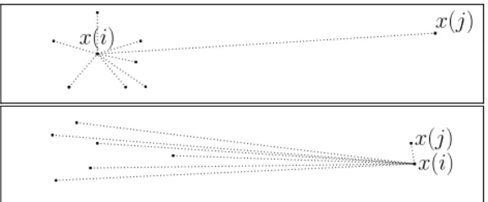
Figure 1: Using the inequality E(j) ≥ |E(i) −
dist(x(i), x(j))| to eliminate x(j) as a medoid candi-date. Computed elementx(i) with energyE(i)≥Ecl
is used as a pivot to lower bound E(j). The two cases where the inequality is effective are when (case 1, above) dist(x(i), x(j))−E(i) ≥ Ecl and (case 2,
below) E(i)−dist(x(i), x(j))≥ Ecl, as both lead to E(j)≥Ecl which eliminatesx(j) as a medoid
candi-date.
Proof. We need to prove that l(j)≤E(j) for allj ∈ {1, . . . , N} at all iterations of the algorithm. Clearly, asl(j) = 0 at initialisation, we havel(j)≤E(j) at ini-tialisation. E(j) does not change, and the only time that l(j) may change is on line 13, where we need to check that|l(i)−d(j)| ≤E(j). At line 13,l(i) =E(i) from line 8, andd(j) = dist(x(i), x(j)), so at line 13 we are effectively checking that |E(i)−dist(x(i), x(j))| ≤ E(j). But this is a simple consequence of the trian-gle inequality, as we now show. Using the definition,
E(j) = N1 PN
l=1dist(x(l), x(j)), we have on the one
hand, E(j)≥ 1 N N X l=1 dist(x(l), x(i))−dist(x(i), x(j)) ≥E(i)−dist(x(i), x(j)), (4) and on the other hand,
E(j)≥ 1 N N X l=1 dist(x(i), x(j))−dist(x(l), x(i)) ≥dist(x(i), x(j))−E(i). (5) Combining (4) and (5) we obtain the required inequal-ity |E(i)−dist(x(i), x(j))| ≤E(j).
The bound test (line 4) becomes more effective at later iterations, for two reasons. Firstly, whenever an ele-ment is computed, the lower bounds of other samples may increase. Secondly, Ecl will decrease whenever a
better medoid candidate is found. The main result of this paper, presented as Theorem 3.2, is that in Rd
the expected number of computed elements isO(N12)
theO(N12) result holds even in settings where the
as-sumptions are not valid or relevent, such as for network data.
The shuffle on line 3 is performed to avoid w.h.p. pathological orderings, such as when elements are or-dered in descending order of energy which would result in all N elements being computed.
Theorem 3.2. Let S ={x(1), . . . , x(N)} be a set of
N elements inRd, drawn independently from
probabil-ity distribution function fX. Let the medoid of S be
x(m∗), and let E(m∗) = E∗. Suppose that there ex-ist strictly positive constants ρ, δ0andδ1 such that for
any set sizeN with probability 1−O(1/N)
x∈ Bd(x(m∗), ρ) =⇒ δ0≤fX(x)≤δ1, (6)
where Bd(x, r) = {x0 ∈ Rd : kx0−xk ≤ r}. Let
α >0be a constant (independent ofN) such that with probability1−O(1/N) alli∈ {1, . . . , N} satisfy,
x(i)∈ Bd(x(m∗), ρ) =⇒ (7) E(i)−E∗≥αkx(i)−x(m∗)k2.
Then, the expected number of elements computed by
trimed is OVd[1]δ1+d α4 d N12 , whereVd[1] = πd2/(Γ(d 2+ 1))is the volume ofBd(0,1).
3.1 On the assumptions in Theorem 3.2 The assumption of constantsρ, δ0andδ1made in
The-orem 3.2 is weak, and only pathological distributions might fail it, as we now discuss. For the assumptions to fail requires thatfX vanishes or diverges at the distri-bution medoid. Any reasonably behaved distridistri-bution does not have this behaviour, as illustrated in Figure 2. The constantαis a strong convexity constant. The ex-istence ofα >0 is guaranteed by the existence ofρ, δ0
andδ1, as the mean of a sum of uniformly spaced cones
converges to a quadratic function. This is illustrated in 1-D in Figure 5 in SM-G, but holds true in any dimension.
Note that the assumptions made are on the distribu-tion fX, and not on the data itself. This must be so in order to prove complexity results inN.
3.2 Sketch of proof of Theorem 3.2
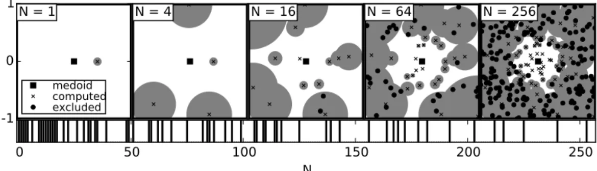
We now sketch the proof of Theorem 3.2, showing how (6) and (7) are used. A full proof is presented in SM-G. Firstly, let the index of the first element after the shuffle on line 3 be i0. Then, no elements beyond radius 2E(i0) of x(i0) will subsequently be computed, due to type 1 eliminations (see Figure 1). Therefore, all computed elements are contained within
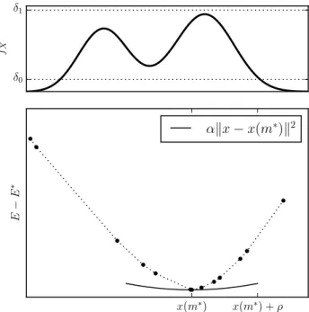
Bd(x(i0),2E(i0)). δ0 δ1 fX x(m∗) x(m∗) +ρ E − E ∗ αkx−x(m∗)k2
Figure 2: Illustration in 1-D of the constants used in Theorem 3.2. Above,δ0andδ1bound the probability
density function in a region containing the distribution medoid. Below, the energy of samples grows quadrati-cally around the medoidx(m∗). The energyEis a sum of cones centered on samples, which is approximately quadratic unless fX vanishes or explodes, guarantee-ing the existence of α >0 required in Theorem 3.2.
Next, notice that once an element x(i) has been computed in trimed, no elements in the ball
Bd(x(i), E(i)−Ecl) will subsequently be computed,
due to type 2 eliminations (see Figure 1). We refer to such a ball as anexclusion ball. By upper bounding the number of exclusion balls contained inBd(x(i0),2E(i0))
using a volumetric argument, we can obtain a bound on the number of computed elements, but obtaining such an upper bound requires that the radii of exclu-sion ballE(i)−Eclbe bounded below by a strictly pos-itive value. However, by using a volumetric argument only beyond a certain positive radius of the medoid (a radius N−1/2d), we haveα > 0 in (15) which
pro-vides a lower bound on exclusion ball radii, assuming
Ecl ≈E∗. Using δ
0 we can show that Ecl approaches E∗ sufficiently fastsufficiently fast to validate the ap-proximationEcl≈E∗.
It then remains to count the number of computed elements within radius N−1/2d of the medoid. One
cannot find a strict upper bound here, but using the boundedness offXprovided byδ1, we have w.h.p. that
the number of elements computed within N−1/2d is
O(δ1N1/2), as the volume of a sphere scales as the d’th power of its radius.
4
Our accelerated
K
-medoids
algorithm :
trikmeds
We adapt our new medoid algorithmtrimedand bor-row ideas from Elkan (2003) to show how KMEDS can be accelerated. We abandon the initial N2 distance
calculations, and only compute distances when nec-essary. The accelerated version of lloyd of Elkan (2003) maintains KN bounds on distances between points and centroids, allowing a large proportion of distance calculations to be eliminated. We use this approach to accelerate assignment in trikmeds, in-curring a memory cost O(KN). By adopting the algorithm of Newling and Fleuret (2016a) or that of Hamerly (2010), the memory overhead can be re-duced toO(N). We accelerate the medoid update step by adapting trimed, reusing lower bounds between it-erations, so thattrimedis only run from scratch once at the start. Details and pseudocode are presented in SM-H.
One can relax the bound test in trimed so that for
>0 elementiis computed if l(i)(1 +)< Ecl,
guar-anteeing that an element with energy within a factor 1 + of E∗ is found. It is also possible to relax the bound tests in the assignment step of trikmeds, such that the distance to an assigned cluster’s medoid is al-ways within a factor 1+of the distance to the nearest medoid. We denote by trikmeds- the trikmeds al-gorithm where the update and assignment steps are relaxed as just discussed, with trikmeds-0 being ex-actly trikmeds. The motivation behind such a relax-ation is that, at all but the final few iterrelax-ations, it is probably a waste of computation obtaining medoids and assignments at high resolution, as in subsequent iterations they may change.
5
Results
We first compare the performance of the medoid algo-rithmsTOPRANK,TOPRANK2andtrimed. We then com-pare theK-medoids algorithms,KMEDSandtrikmeds.
5.1 Medoid algorithm results
We compare our new exact medoid algorithmtrimed
with state-of-the-art approximate algorithmsTOPRANK
and TOPRANK2. Recall, Okamoto et al. (2008) prove that the approximate algorithms return w.h.p. the true medoid. We confirm that this is the case in all our ex-periments, where the approximate algorithms return the same element as trimed, which we know to be correct by Theorem 3.1. We now focus on compar-ing computational costs, which are proportional to the number of computed points.
Results on artificial datasets are presented in Figure 3, where our two main observations relate to scaling in
N and dimension d. The artificial data are (left) uniformly drawn from [0,1]d and (right) drawn from Bd(0,1) with probability of lying within radius 1/21/d
of 1/200, as opposed to 1/2 as would be the case under uniform density. Details about sampling from this dis-tribution can be found in SM-F. Results on a mix of publicly available real and artificial datasets are pre-sented in Table 1 and discussed in§5.1.2.
5.1.1 Scaling with N and don artificial datasets
In Figure 3 we observe that the number of points com-puted by trimed is O(N1/2), as predicted by
Theo-rem 3.2. This is illustrated (right) by the close fit of the number of computed points to exact square root curves at sufficiently large N ford∈ {2,6}.
Recall that TOPRANK consists of two passes, a first whereN2/3log1/3N anchor points are computed, and a second where all sub-threshold points are computed. We observe that for small N TOPRANK computes all
N points, which corresponds to all points lying be-low threshold. At sufficiently large N the threshold becomes low enough for all points to be eliminated af-ter the first pass. The effect is particularly dramatic in high dimensions (d = 6 on right), where a phase transition is observed between all and no points being computed in the second pass.
Dimensiondappears in Theorem 3.2 through a factor
d(4/α)d, whereαis the strong convexity of the energy
at the medoid. In Figure 3, we observe that the num-ber of computed points increases with d for fixed N, corresponding to a relatively small α. The effect of α
on the number of computed elements is considered in greater detail in SM-F.
In contrast to the above observation that the number of computed points increases as dimension increases fortrimed,TOPRANKappears to scale favourably with dimension. This observation can be explained in terms of the distribution of energies, with energies close toE∗
being less common in higher dimensions, as discussed in SM-J.
5.1.2 Results on publicly available real and simulated datasets
We present the datasets used here in detail in SM-I. For all datasets, algorithms TOPRANK, TOPRANK2 and
trimed were run 10 times with a distinct seed, and the mean number of iterations (ˆn) over the 10 runs was computed. We observe that our algorithmtrimed
is the best performing algorithm on all datasets, al-though in high-dimensions (MNIST-0) and on social
102 103 104 105 106 N 102 103 104 105 106 number of computed elements TOPRANK trimed d= 2 d= 3 d= 4 d= 5 d= 6 103 104 105 106 107 N 102 103 104 105 106 N 18N12 N23log 1 3N 3N12 d= 2TOPRANK d= 2trimed d= 6TOPRANK d= 6trimed
Figure 3: Comparison of TOPRANKand our algorithmtrimedon simulated data. On the left, points are drawn uniformly from [0,1]d for d∈ {2, . . . ,6}, and on the right they are drawn from B
d(0,1) ford∈ {2,6}, with an
increased density near the edge of the ball. Fewer points (elements) are computed by trimedthan byTOPRANK
in all scenarios. For smallN,TOPRANKcomputesO(N) points, before transitioning to ˜O(N2/3) computed points
for large N. trimedcomputesO(N1/2) points. Note thattrimedperforms better in low-dthan in high-d, with
the reverse trend being true for TOPRANK. These observations are discussed in further detail in the text.
network data (Gnutella) no algorithm computes sig-nificantly fewer than N elements. The failure in high-dimensions (MNIST-0) of trimed is in agree-ment with Theorem 3.2, where dimension appears as the exponent of a constant term. The small world network data, Gnutella, can be embedded in a high-dimensional Euclidean space, and thus the failure on this dataset can also be considered as being due to high-dimensions. For low-dimensional real and spatial network data,trimed consistently computesO(N1/2) elements.
5.1.3 But who needs the exact medoid anyway?
A valid criticism that could be raised at this stage would be that for large datasets, finding the exact medoid is probably overkill, as any point with en-ergy reasonably close to E∗ suffices for most
appli-cations. But consider, the RAND algorithm requires computing logN/2 elements to confidently return an
element with energy within E∗ of E∗. ForN = 105
and = 0.05, this is 4600, already more thantrimed
requires to obtain the exact medoid on low-ddatasets of comparable size.
5.2 K-medoids algorithm results
WithN elements to cluster,KMEDSis Θ(N2) in
mem-ory, rendering it unusable on even moderately large datasets. To compare the initialisation scheme pro-posed in Park and Jun (2009) to random initialisation, we have performed experiments on 14 small datasets, with K ∈ {10,dN1/2e,dN/10e}. For each of these 42
experimental set-ups, we run the deterministic KMEDS
initialisation once, and then uniform random initial-isation, 10 times. Comparing the mean final energy of the two initialisation schemes, in only 9 of 42 cases does KMEDS initialisation result in a lower mean final energy. A Table containing all results from these ex-periments in presented in SM-E.
Having demonstrated that random uniform initiali-sation performs at least as well as the initialiinitiali-sation scheme ofKMEDS, and noting thattrikmeds-0returns exactly the same clustering as would KMEDSwith uni-form random initialisation, we turn our attention to the computational performance of trikmeds. Table 2 presents results on 4 datasets, each described in SM-I. The first numerical column is the relative number of distance calculations using trikmeds-0andKMEDS, where large savings in distance calculations, especially in low-dimensions, are observed. Columns φc andφE
are the number of distance calculations and energies respectively, using ∈ {0.01,0.1}, relative to = 0. We observe large reductions in the number of distance computations with only minor increases in energy.
6
Conclusion and future work
We have presented our newtrimedalgorithm for com-puting the medoid of a set, and provided strong the-oretical guarantees about its performance in Rd. In
low-dimensions, it outperforms the state-of-the-art ap-proximate algorithm on a large selection of datasets. The algorithm is very simple to implement, and can easily be extended to the general ranking problem. In the future, we propose to explore the idea of
us-TOPRANK TOPRANK2 trimed
dataset type N nˆ nˆ nˆ
Birch 1 2-d 1.0×10⁵ 57944 100180 2180
Birch 2 2-d 1.0×10⁵ 66062 100180 2208
Europe 2-d 1.6×10⁵ 176095 169535 2862
U-Sensor Net u-graph 3.6×10⁵ 113838 327216 1593 D-Sensor Net d-graph 3.6×10⁵ 99896 176967 1372 Pennsylvania road u-graph 1.1×10⁶ 216390 time-out 2633
Europe rail u-graph 4.6×10⁴ 35913 47041 518
Gnutella d-graph 6.3×10³ 7043 6407 6328
MNIST 784-d 6.7×10³ 7472 6799 6514
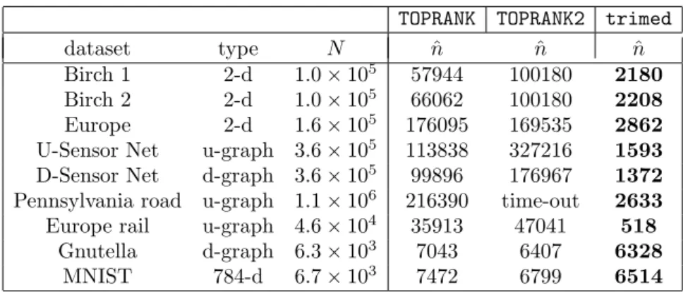
Table 1: Comparison of TOPRANK,TOPRANK2and our algorithmtrimedon publicly available real and simulated datasets. Column 2 provides the type of the dataset, where ‘x-d’ denotes x-dimensional vector data, while ‘d-graph’ and ‘u-graph’ denote directed and undirected graphs respectively. Column ˆngives the mean number of elements computed over 10 runs. Our proposed trimed algorithm obtains the true medoid with far fewer computed points in low dimensions and on spatial network data. On the social network dataset (Gnutella) and the very high-ddataset (MNIST), all algorithms fail to provide speed-up, computing approximatelyN elements.
K= 10 K=d√Ne = 0 = 0.01 = 0.1 = 0 = 0.01 = 0.1 Dataset N d Nc/N2 φc φE φc φE Nc/N2 φc φE φc φE Europe 1.6×10⁵ 2 0.067 0.33 1.004 0.01 1.054 0.008 0.68 1.031 0.39 1.090 Conflong 1.6×10⁵ 3 0.042 0.67 1.001 0.08 1.014 0.006 0.92 1.003 0.61 1.026 Colormo 6.8×10⁴ 9 0.163 0.92 1.000 0.35 1.015 0.011 0.98 1.000 0.82 1.005 MNIST50 6.0×10⁴ 50 0.280 0.99 1.000 0.95 1.001 0.019 0.99 1.001 0.97 1.001
Table 2: Relative numbers of distance calculations and final energies usingtrikmeds-for∈ {0,0.01,0.1}. The number of distance calculations with trikmeds-0 isNc, presented here relative to the number computed using
KMEDS (N2) in columnN
c/N2. The number of distance calculations with∈ {0.01,0.1} relative totrikmeds-0
are given in columns φc, so φc = 0.33 means 3× fewer calculations than with = 0. The final energies with
∈ {0.01,0.1}relative totrikmeds-0are given in columnsφE. We see thattrikmeds-0uses significantly fewer distance calculations than would KMEDS, especially in low-dimensions where a greater than K× reduction is observed (NC/N2<1/K). For low-d, additional relaxation further increases the saving in distance calculations
with little cost to final energy.
ing more complex triangle inequality bounds involving several points, with as goal to improve on theO(N1/2)
number of computed points.
We have demonstrated how trimed, when combined with the approach of Elkan (2003), can greatly reduce the number of distance calculations required by the Voronoi iteration K-medoids algorithm of Park and Jun (2009). In the future we would like to replace the strategy of Elkan (2003) with that of Hamerly (2010), which will be better adapted to graph clustering as either all or no distances are computed with it, making it more amenable to Dijkstra’s algorithm.
Acknowledgements
The authors are grateful to Wei Chen for helpful dis-cussions of the TOPRANK algorithm. James Newling was funded by the Hasler Foundation under the grant 13018 MASH2.
References
Arthur, D. and Vassilvitskii, S. (2007). K-means++: The advantages of careful seeding. InProceedings of the Eighteenth Annual ACM-SIAM Symposium on Discrete Algorithms, SODA ’07, pages 1027–1035, Philadelphia, PA, USA. Society for Industrial and Applied Mathematics.
Statistical Analysis of Gene Expression Microarray Data. Chapman & Hall. Chapter 4.
Cohen, E., Delling, D., Pajor, T., and Werneck, R. F. (2014). Computing classic closeness centrality, at scale. InProceedings of the Second ACM Conference on Online Social Networks, COSN ’14, pages 37–50, New York, NY, USA. ACM.
Cohen, M. B., Lee, Y. T., Miller, G. L., Pachocki, J. W., and Sidford, A. (2016). Geometric median in nearly linear time. In STOC16. submitted.
Elkan, C. (2003). Using the triangle inequality to ac-celerate k-means. InMachine Learning, Proceedings of the Twentieth International Conference (ICML 2003), August 21-24, 2003, Washington, DC, USA, pages 147–153.
Eppstein, D. and Wang, J. (2004). Fast approximation of centrality.J. Graph Algorithms Appl., 8(1):39–45. Frahm, J.-M., Fite-Georgel, P., Gallup, D., Johnson, T., Raguram, R., Wu, C., Jen, Y.-H., Dunn, E., Clipp, B., Lazebnik, S., and Pollefeys, M. (2010). Building rome on a cloudless day. InProceedings of the 11th European Conference on Computer Vision: Part IV, ECCV’10, pages 368–381, Berlin, Heidel-berg. Springer-Verlag.
Hamerly, G. (2010). Making k-means even faster. In
SDM, pages 130–140.
Hastie, T. J., Tibshirani, R. J., and Friedman, J. H. (2001). The elements of statistical learning : data mining, inference, and prediction. Springer series in statistics. Springer, New York.
Hoare, C. A. R. (1961). Algorithm 65: Find.Commun. ACM, 4(7):321–322.
Kaufman, L. and Rousseeuw, P. J. (1990). Finding groups in data : an introduction to cluster analy-sis. Wiley series in probability and mathematical statistics. Wiley, New York. A Wiley-Interscience publication.
Newling, J. and Fleuret, F. (2016a). Fast k-means with accurate bounds. In Proceedings of the Inter-national Conference on Machine Learning (ICML), pages 936–944.
Newling, J. and Fleuret, F. (2016b). K-medoids for k-means seeding. arXiv:1609.04723. Under review. Ng, R. T., Han, J., and Society, I. C. (2005). Clarans:
A method for clustering objects for spatial data min-ing. IEEE Transactions on Knowledge and Data Engineering, pages 1003–1017.
Okamoto, K., Chen, W., and Li, X.-Y. (2008). Rank-ing of closeness centrality for large-scale social net-works. In Proceedings of the 2Nd Annual Interna-tional Workshop on Frontiers in Algorithmics, FAW ’08, pages 186–195, Berlin, Heidelberg. Springer-Verlag.
Park, H.-S. and Jun, C.-H. (2009). A simple and fast algorithm for k-medoids clustering.Expert Syst. Appl., 36(2):3336–3341.
Rattigan, M. J., Maier, M., and Jensen, D. (2007). Graph clustering with network structure indices. In
Proceedings of the 24th International Conference on Machine Learning, ICML ’07, pages 783–790, New York, NY, USA. ACM.
SM-A
On the difficulty of the medoid problem
We construct an example showing that no general purpose algorithm exists to solve the medoid problem in
o(N2). Consider an almost fully connected graph containingN = 2m+ 1 nodes, where the graph is exactlym
edges short of being fully connected: one node has 2medges and the others have 2m−1 edges. The graph has 2m2edges. With the shortest path metric, it is easy to see that the node with 2medges is the medoid, hence the medoid problem is as difficult as finding the node with 2medges. But, supposing that the edges are provided as an unsorted adjacency list, it is clearly an O(m2) task to determine which node has 2medges as one must look
at all edges until a node with 2medges is found. Thus determining the medoid isO(m2) which isO(N2).
SM-B
KMEDS
pseudocode
Alg. 2 presents the KMEDS algorithm of Park and Jun (2009), with the novel initialisation of KMEDS on line 1.
KMEDS is essentiallylloyd, with medoids instead of means.
Algorithm 2KMEDSfor clustering data{x(1), . . . , x(N)} aroundKmedoids
1: Set all distancesD(i, j)← kx(i)−x(j)k and sumsS(i)←P
j∈{1,...,N}D(i, j) 2: Initialise medoid indices asKindices minimisingf(i) =P
j∈{1,...,N}D(i, j)/S(j) 3: whileSome convergence criterion has not been metdo
4: Assign each element to the cluster whose medoid is nearest to the element
5: Update cluster medoids according to assignments made above
6: end while
SM-C
RAND
,
TOPRANK
and
TOPRANK2
pseudocode
We present pseudocode for the RAND, TOPRANKand TOPRANK2algorithms of Okamoto et al. (2008), and discuss the explicit and implicit constants.
SM-C.1 On the number of anchor elements in TOPRANK: the constant in Θ(N23(logN) 1 3)
Note that the number of anchor points used in TOPRANK does not affect the result that the medoid is w.h.p. returned. However, Okamoto et al. (2008) show that by choosing the size of the anchor set to beq(logN)13 for
any q, the run time is guaranteed to be ˜O(N5/3). They do not suggest a specificq, the optimalq being dataset
dependant. We chooseq= 1.
Consider Figure 3 in Section 5.1 for example, where q = 1. Had q be chosen to be less than 1, the line
ncomputed=N2/3log1/3
N to whichTOPRANK runs parallel for large N would be shifted up or down by logq, however the N at which the transition from ncomputed=N2/3log1/3
N to ncomputed =N2/3log1/3
N takes place would also change.
SM-C.2 On the parameter α0 in TOPRANK and TOPRANK2
The thresholdτ in (2) is proportional to the parameterα0. In Okamoto et al. (2008), it is stated thatα0 should be some value greater than 1. Note that the smallerα0is, the lower the threshold is, and hence fewer the number of computed points is, thus α0 = 1.00001 would be a fair choice. We useα0 = 1 in our experiments, and observe that the correct medoid is returned in all experiments.
Personal correspondence with the authors of Okamoto et al. (2008) has brought into doubt the proof of the result that the medoid is w.h.p. returned for any α0 where α0 > 1. In our most recent correspondence, the authors suggest that the w.h.p. result can be proven with the more conservative bound of α0 >√1.5. Moreover, we show in SM-D that α0 >1 is good enough to return the medoid with probability N−(α0−1), a probability which still tends to 0 asN grows large, but not a w.h.p. result. Please refer to SM-D for further details on our correspondence with the authors.
SM-C.3 On the parameters specific to TOPRANK2
In addition to α0,TOPRANK2requires two parameters to be set. The first isl0, the starting anchor set size, and
the second is q, the amount by which l should be incremented at each iteration. Okamoto et al. (2008) suggest taking l0 to be the number of top ranked nodes required, which in our case would bel0 =k = 1. However, in
our experience this is too small as all nodes lie well within the threshold and thus when l increases there is no change to number below threshold, which makes the algorithm break out of the search for the optimalltoo early. Indeed,l0 needs to be chosen so that at least some points have energies greater than the threshold, which in our
experiments is already quite large. We choose l0 = √
N, as any value larger thanN2/3 would make TOPRANK2
redundant to TOPRANK. The parameter qwe take to be logN as suggested by Okamoto et al. (2008). Algorithm 3RANDfor estimating energies of elements of setS (Eppstein and Wang, 2004).
I←random uniform sample from{1, . . . , N}
// Compute all distances from anchor elements (I), using Dijkstra’s algorithm on graphs
fori∈Ido
forj∈ {1, . . . , N} do
d(i, j)← kx(i)−x(j)k, end for
end for
// Estimate energies as mean distances to anchor elements
forj∈ {1, . . . , N} do ˆ E(j)← 1 |I| P i∈Id(i, j) end for return Eˆ
Algorithm 4TOPRANKfor obtaining topkranked elements ofS (Okamoto et al., 2008).
l←N23(logN) 1
3 // Okamoto et al. (2008) state thatlshould be Θ((logN) 1
3), the choice of 1 as the constant
is arbitrary (see comments in the text of Section SM-C.1).
RunRANDwith uniform randomI of sizel to get ˆE(i) fori∈ {1, . . . , N}.
Sort ˆE so that ˆE[1]≤Eˆ[2]≤. . .≤Eˆ[N] ˆ
∆←2 mini∈Imaxj∈{1,...,N}kx(i)−x(j)k // wherekx(i)−x(j)k computed inRAND Q← i∈ {1, . . . , N} |Eˆ(i)≤Eˆ[k] + 2α0∆ q log(n) l .
Compute exact energies of all elements inQand return the element with the lowest energy.
SM-D
On the proof that
TOPRANK
returns the medoid with high probability
Through correspondence with the authors of Okamoto et al. (2008), we have located a small problem in the proof that the medoid is returned w.h.p. for α0 >1, the problem lying in the second inequality of Lemma 1. To arrive at this inequality, the authors have used the fact that for alli,
P(E(i)≥Eˆ(i) +f(l)·∆)≥1−
1
2N2, (8)
which is a simple consequence of the Hoeffding inequality as shown in Eppstein and Wang (2004). Essentially (8) says that, for a fixed node i, from which the mean distance to other nodes isE(i), if one uniformly samples l
distances to i and computes the mean ˆE(i), the probability that ˆE(i) is less than E(i) +f(l) is greater than 1− 1
2N2.
The inequality (8) is true for a fixed nodei. However, it no longer holds ifiis selected to be the node with the lowest ˆE(i). To illustrate this, suppose thatE(i) = 1 for alli, and compute ˆE(i) for alli. Let ˆE∗= arg miniEˆ(i). Now, we have a strong prior on ˆE∗ being significantly less than 1, and (8) no longer holds as a statement made about ˆE∗.
In personal correspondence, the authors show that the problem can be fixed by the use of an additional layer of union bounding, with a correction to be published (if not already done so at time of writing). However, the
Algorithm 5TOPRANK2for obtaining topkranked elements ofS (Okamoto et al., 2008).
// In Okamoto et al. (2008), it is suggested thatl0be taken as k, which in the case of the medoid problem is
1. We have experimented with several choices for l0, as discussed in the text. l←l0
RunRANDwith uniform randomI of sizel to get ˆE(i) fori∈ {1, . . . , N}.
ˆ
∆←2 mini∈Imaxj∈{1,...,N}kx(i)−x(j)k // wherekx(i)−x(j)k computed inRAND
Sort ˆE so that ˆE[1]≤Eˆ[2]≤. . .≤Eˆ[N] Q← i∈ {1, . . . , N} |Eˆ(i)≤Eˆ[k] + 2α0∆ q log(n) l . g←1 while gis 1 do p← |Q|
// The recommendation for qin Okamoto et al. (2008) is log(n), we follow the suggestion
IncrementI withqnew anchor points
Update ˆE for all data according to new anchor points
l← |I|
ˆ
∆←2 mini∈Imaxj∈{1,...,N}kx(i)−x(j)k
Sort ˆE so that ˆE[1]≤Eˆ[2]≤. . .≤Eˆ[N] Q← i∈ {1, . . . , N} |Eˆ(i)≤Eˆ[k] + 2α0∆ q log(n) l p0← |Q| if p−p0 <log (n)then g←0 end if end while
Compute exact energies of all elements inQand return the element with the lowest energy
additional layer of union bound requires a more conservative constraint on α0, which is α0 >2, although the authors propose that the w.h.p. result can be proven with α0 >√1.5 forN sufficiently large. We now present a small proof proving the w.h.p. result for α0 > √2 for N sufficiently large, with at the same time α0 > 1 guaranteeing that the medoid is returned with probabilityO(Nα0−1).
SM-D.1 That the medoid is returnedwith high probability holds forα0>√2 and that with
vanishing probability it is returned for α0 >1
Recall that we have N nodes with energies E(1), . . . , E(n). We wish to find the k lowest energy nodes (the original setting of Okamoto et al. (2008)). From Hoeffding’s inequality we have,
P(|E(i)−Eˆ(i)| ≥∆)≤2 exp −l2. (9)
Set the probability on the right hand side of 9 to be 2/N1+β, that is, 2 exp −l2 = 2/N1+β, which corresponds to = s 1 +β l log (N) := f˜(l).
Clearly√1 +β corresponds toα0. With this notation we have,
P(|E(i)−Eˆ(i)| ≥f˜(l)∆)≤ 2
N1+β. (10)
Applying the union bound to (10) we have,
P ¬∧i∈{1,...,N}|E(i)−Eˆ(i)| ≤f˜(l)∆ ≤ 2 Nβ. (11)
K= 10 K=l√Nm K=N 10
Dataset N d µu/µpark σu/µpark µu/µpark σu/µpark µu/µpark σu/µpark gassensor 256 128 1.09 0.08 0.90 0.03 0.83 0.01 house16H 1927 17 1.01 0.02 0.97 0.01 0.93 0.01 S1 5000 2 1.05 0.05 0.75 0.01 0.32 0.01 S2 5000 2 1.04 0.07 0.68 0.01 0.34 0.00 S3 5000 2 1.03 0.05 0.76 0.01 0.35 0.00 S4 5000 2 1.02 0.03 0.75 0.01 0.41 0.01 A1 3000 2 0.82 0.03 0.43 0.01 0.19 0.00 A2 5250 2 0.98 0.03 0.47 0.01 0.25 0.00 A3 7500 2 0.96 0.02 0.42 0.02 0.22 0.00 thyroid 215 5 0.95 0.08 0.97 0.04 0.93 0.04 yeast 1484 8 1.00 0.02 0.96 0.02 0.91 0.02 wine 178 14 1.01 0.02 1.02 0.01 0.98 0.02 breast 699 9 0.79 0.03 0.77 0.02 0.68 0.02 spiral 312 3 1.03 0.03 0.99 0.02 0.82 0.03
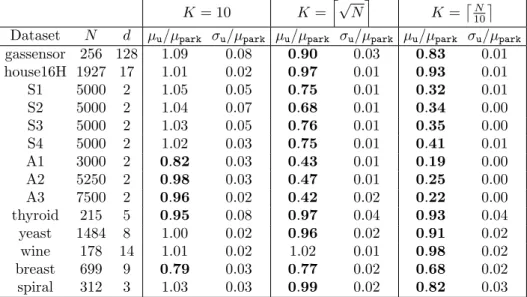
Table 3: Comparing the initialisation scheme proposed in Park and Jun (2009) with random uniform initialisation for the KMEDS algorithm. The final energy using the deterministic scheme proposed in Park and Jun (2009) is
µpark. The mean over 10 random uniform initialisations isµu, and the corresponding standard deviation is σu. For small K (K = 10), the performances using the two schemes are comparable, while for largerK, it is clear that uniform initialisation performs much better on the majority of datasets.
Recall that we wish to obtain the k nodes with lowest energy. Denote by r(j) the index of the node with the
j’th lowest energy, so that
E(r(1))≤. . .≤E(r(j))≤. . .≤E(r(N)).
Denote by ˆr(j) the index of the node with the j’th lowest estimated energy, so that ˆ
E(ˆr(1))≤. . .≤Eˆ(ˆr(j))≤. . .≤Eˆ(ˆr(N)).
Now assume that for alli, it is true that|E(i)−Eˆ(i)| ≤f˜(l). Then consider, forj≤k, ˆ E(ˆr(k))−Eˆ(r(j)) =Eˆ(ˆr(k))−E(r(k)) | {z } ≥−f˜(l)∆ +E(r(k))−E(r(j)) | {z } ≥0 +E(r(j))−Eˆ(r(j)) | {z } ≥−f˜(l)∆ , (12) ≥ −2 ˜f(l)∆.
The first bound in (12) is obtained by considering the most extreme case possible under the assumption, which is ˆE(i) =a(E)−f˜(l) for all i. The second bound follows fromj≤k, and the third bound follows directly from the assumption. We thus have that, under the assumption,
ˆ
E(r(j))≤Eˆ(ˆr(k)) + 2 ˜f(l)∆,
which says that all nodes of rank less than or equal tok have approximate energy less than ˆE(ˆr(k)) + 2 ˜f(l)∆. As the assumption holds with probability greater than 1−2/Nβ by (11), we are done. Takeβ = 1 if you want the statement with high probability, that is
=
r
2 log(n)
l ,
but for any β >0, which corresponds toα0 >1, the probability of failing to return the k lowest energy nodes tends to 0 asN grows.
SM-E
On the initialisation of Park and Jun (2009)
In Table 3 we present the full results of the 48 experiments comparing the initialisation proposed in Park and Jun (2009) with simple uniform initialisation. The 14 datasets are all available from https://cs.joensuu.fi/ sipu/datasets/.
0.0
0.2
0.4
0.6
0.8
1.0
1.2
N
1e6
0.0
0.5
1.0
1.5
2.0
2.5
number of points computed
1e4
7
.
8
pN
10
.
6
pN
15
.
5
pN
22
.
3
pN
d
=2
d
=3
d
=4
d
=5
0.0
0.2
0.4
0.6
0.8
1.0
1.2
N
1e6
0.0
0.2
0.4
0.6
0.8
1.0
1.21e4
3
.
7
pN
5
.
0
pN
7
.
1
pN
11
.
2
pN
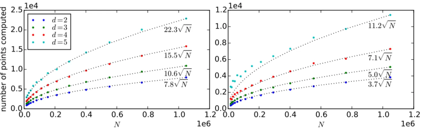
Figure 4: Number of points computed on simulated data. Points are drawn from Bd(0,1), for d∈ {2,3,4,5}.
On the left, points are drawn uniformly, while on the right, the density in Bd(0,(1/2)1/d) is 19× lower that
in Ad(0,(1/2)1/2,1), where recall that Ad(x, r1, r2) denotes an annulus centred at x of inner radius r1 and
outer radius r2. We observe a near perfect fit of the number of computed points toξ √
N where the constant
ξ depends on the dimension and the distribution (left and right). The number of computed points increases with dimension. The strong convexity constant of the distribution on the right is larger, corresponding to fewer distance calculations as predicted by Theorem 3.2.
SM-F
Scaling with
α
,
N
, and dimension
d
We perform more experiments to provide further validation of Theorem 3.2. In particular, we check how the number of computed elements scales withN,dandα. We generate data from a unit ball in various dimensions, according to two density functions with different strong convexity constants α. The first density function is uniform, so that the density everywhere in the ball is uniform. To sample from this distribution, we generate two random variables, X1∼ Nd(0,1) andX2∼U(0,1) and use
X3=X1/kX1k ·X 1
d
2, (13)
as a sample from the unit ball Bd(0,1) with uniform distribution. The second distribution we consider has a
higher density beyond radius (1/2)1/d. Specifically, within this radius the density is 19×lower than beyond this
radius. To sample from this distribution, we sample X3 according to (13), and then points lying within radius
(1/2)1/d are with probability 1/10 re-sampled uniformly beyond this radius.
The second distribution has a larger strong convexity constant α. To see this, note that the strong convexity constant at the center of the ball depends only on the density of the ball on its surface, that is at radius 1, as can be shown using an argument based on cancelling energies of internal points. As the density at the surface under distribution 2 is approximately twice that of under distribution 1, the change in energy caused by a small shift in the medoid is twice as large under distribution 2. Thus, according to Theorem 3.2, we expect the number of computed points to be larger under distribution 1 than under distribution 2. This is what we observe, as shown in Figure 4, where distribution 1 is on the left and distribution 2 is on the right.
In Figure 4 we observe a near perfectN1/2scaling of number of computed points. Dashed curves are exactN1/2
relationships, while the coloured points are the observed number of computed points.
SM-G
Proof of Theorem 3.2 (See page 5)
Theorem 3.2. Let S ={x(1), . . . , x(N)} be a set of N elements in Rd, drawn independently from probability
distribution function fX. Let the medoid ofS bex(m∗), and let E(m∗) =E∗. Suppose that there exist strictly positive constants ρ, δ0 andδ1 such that for any set sizeN with probability 1−O(1/N)
whereBd(x, r) ={x0 ∈Rd : kx0−xk ≤r}. Letα >0be a constant (independent ofN) such that with probability
1−O(1/N)alli∈ {1, . . . , N} satisfy,
x(i)∈ Bd(x(m∗), ρ) =⇒ (7)
E(i)−E∗≥αkx(i)−x(m∗)k2.
Then, the expected number of elements computed by trimed is OVd[1]δ1+d α4
d N12 , where Vd[1] = πd2/(Γ(d 2+ 1))is the volume ofBd(0,1).
Proof. We show that the assumptions made in Th. 3.2 validate the assumptions required in Thm SM-G.1. Firstly, if e(i)> ρthene(i)≥αρ2e(i)> ρ, which follows from the convexity of the loss function and. Secondly,
the existance of β follows from continuity of the gradient of the distance, combined with the existence of δ1
(non-exploding).
Theorem SM-G.1 (Main Theorem Expanded). LetS ={x(1), . . . , x(N)} ⊂Rd have medoidx(m∗)with
min-imum energy E(m∗) =E∗, where elements inS are drawn independently from probability distribution function
fX. Let e(i) = kx(i)−x(m∗)k. Suppose that for fX there exist strictly positive constants α, β, ρ, δ0 and δ1
satisfying,
x∈ Bd(x(m∗), ρ) =⇒ δ0≤fX(x)≤δ1, (14)
where Bd(x, r) ={x0 ∈Rd : kx0−xk ≤r}, and that for any set size N, w.h.p. all i∈ {1, . . . , N} satisfy,
E(i)−E∗≥ ( αe(i)2 if e(i)≤ρ, αρ2 if e(i)> ρ, (15) and, E(i)−E∗≤βe(i)2 if e(i)≤ρ. (16)
Then the expected number of elements computed, which is to say not eliminated on line 4 of trimed, is
OVd[1]δ1+d 4α d N12 , whereVd[1] =πd2/(Γ(d 2+ 1)) is the volume ofBd(0,1). x(m∗) E−E∗
Figure 5: A sum of uniformly distributed cones is approximately quadratic.
Proof. We first show that the expected number of computed elements in Bd(x(m∗), N− 1
2d) is O(Vd[1]δ1N12).
When N is sufficiently large, fX(x) ≤ δ1 within Bd(x(m∗), N− 1
2d). The expected number of samples in
Bd(x(m∗), N− 1
2d) is thus upper bounded by δ1 multiplied by the volume of the ball. But the volume of a
ball of radiusN−1
2d in Rd isVd[1]N−
1 2.
In Lemma SM-G.2 we use a packing argument to show that the number of computed elements in the annulus
Ad(x(m∗), N− 1 2d,∞) is O d α4d N12
, but we there assume that the medoid indexm∗ is the first element in
shuffle({1, . . . , N}) on line 3 of trimed and thus that the medoid energy is known from the first iteration (Ecl=E∗). We now extend Lemma SM-G.2 to the case where the medoid is not the first element processed. We
do this by showing that w.h.p. an element with energy very close toE∗has been computed afterN−12 iterations
of trimed, and thus that the bounds on numbers of computed elements obtained using the packing arguments underlying Lemma SM-G.2 are all correct to within some small factor afterN−12 iterations.
0
.
4
−
ρ
0
.
0
ρ
0
.
4
k
x
(
i
)
−
x
(
m
∗)
k
αρ
20
.
06
0
.
12
E
(
i
)
−
E
∗Figure 6: Illustrating the parametersα,βandρof Theorem 3.2. Here we drawN = 101 samples uniformly from [−1,1] and compute their energies, plotted here as the series of points. Theorem 3.2 states that their exists α,
β andρsuch that irrespective ofN, all energies (points) will lie in the envelope (non-hatched region).
The probability of a sample lying within radius N−32d ofx(m∗) is Ω(δ0N−23), and so the probability that none
of the first N12 samples lies within radius N− 2 3d isO((1−δ0N− 2 3d)N 1 2) which is O(1 N). Thus w.h.p. afterN 1 2
iterations of trimed, Ecl is within βN−4
3d ofE∗, which means that the radii of the balls used in the packing
argument are overestimated by at most a factorN−31d. Thus w.h.p. the upper bounds obtained with the packing
argument are correct to within a factor 1 +N−13. The remainingO(1
N) cases do not affect the expectation, as
we know that no more than N elements can be computed.
Lemma SM-G.2 (Packing beyond the vanishing radius). If we assume (15) from Theorem 3.2 and that the medoid index m∗ is the first element processed by trimed, then the number of elements computed in Ad(x(m∗), N− 1 2d,∞) isO d α4d N12 .
Proof. Follows from Lemmas SM-G.3 and SM-G.4.
Lemma SM-G.3 (Packing from the vanishing radius N−1
d to ρ). If we assume (15) from Theorem 3.2 and
that the medoid index m∗ is the first element processed in trimed, then the number of computed elements in A(x(m∗), N−21d, ρ)isO(d 4
α
d
N12).
Proof. According to Assumption 15, an element at radius r < ρhas surplus energy at least αr2. This means
that, assuming that the medoid has already been computed, an element computed at radiusrwill be surrounded by an exclusion zone of radius αr2 in which no element will subsequently be computed. We will use this fact
to upper bound the number of computed elements in A(x(m∗), N−21d, ρ), firstly by bounding the number in an
annulus of inner radius r and width αr2, that is the annulus A
d(x(m∗), r, r+αr2), and then summing over
concentric rings of this form which cover A(x(m∗), N−21d, ρ). Recall that the number of computed elements in
We use Lemma SM-G.5 to boundNc(x(m∗), r, r+αr2), Nc(x(m∗), r, r+αr2)≤(d+ 1)2 4 √ 3 d αr2(r+αr2)d−1 (αr2)d ≤(d+ 1)2 4 √ 3 d 1 + 1 αr d−1 ≤(d+ 1)2 4 √ 3 d max 2, 2 αr d−1 ≤(d+ 1)2 4 √ 3 d max 2d−1, 2 αr d−1!! ≤(d+ 1)2 4 √ 3 d 2d−1+ 2 αr d−1! ≤(d+ 1)2 8 √ 3 d + (d+ 1)2 8 √ 3 d 1 αr d−1 Let r0 =N− 1 2d and ri+1=ri+αr2
i, and letT be the smallest indexisuch that ri≤ρ. With this notation in
hand, we have Nc(x(m∗), N− 1 2d, ρ)≤ T X i=0 Nc(x(m∗), ri, αri+ri2).
The summation on the right-hand side can be upper-bounded by an integral. Using that the difference between
ri andri+1 isαr2i, we need to divide terms in the sum byαr2i when converting to an integral. Doing this, we
obtain, Nc(x(m∗), N− 1 2d, ρ)≤ Z ρ+αρ2 N−21d Nc(x(m∗), r, αr2)dr ≤const + (d+ 1)2 8 √ 3 d1 α dZ ∞ N−21d r−(1+d)dr ≤const + (d+ 1) 4 α d N12.
This completes the proof, and provides the hidden constant of complexity as (d+ 1) α4d. Thus larger values for αshould result in fewer computed elements in the annulus Ad(x(m∗), r, r+αr2), which makes sense given
that large values of αimply larger surplus energies and thus larger elimination zones.
Lemma SM-G.4 (Packing beyond ρ). If we assume (15)from Theorem 3.2 and that the medoid index m∗ is the first element processed by trimed, then the number of computed elements in Ad(x(m∗), ρ,∞) is less than
(1 + 4E∗/(αρ2))d.
Proof. Recall that we at assumingm∗= 1, that is that the medoid is the first element processed intrimed. All
elements beyond radius 2E∗ are eliminated by type 1 eliminations (Figure 1), which provides the first inequality
below. Then, as the excess energy is at least = αρ2 for all elements beyond radius ρ of x(m∗), we apply
Lemma SM-G.8 with=αρ2/2 to obtain the second inequality below, Nc(m(x), ρ,∞)≤Nc(m(x), ρ,2E∗) ≤ (2E ∗+1 2αρ 2)d (1 2αρ 2)d ≤ 1 + 4E ∗ αρ2 d .
Lemma SM-G.5 (Annulus packing). For0≤rand0< ≤w. If X ⊂ Ad(0, r, r+w), where ∀x∈ X,Bd(x, )∪ X ={x}, (17) then, |X | ≤(d+ 1)2 4 √ 3 dw(r+w)d−1 d .
Proof. The condition (17) implies,
∀x, x0 ∈ X × X,Bx, 2 ∪ Bx0, 2 =∅. (18)
Using that ∈(0, w] and Lemma SM-G.6, one can show that for allx∈ A(0, r, r+w),
volumeBx, 2 ∩ A(0, r, r+w)> 1 d+ 1 3 4 d2 Vdh 2 i (19)
Combining (18) with (19) we have,
volume [ x∈X Bx, 2 ∩ A(0, r, r+w) ! >Vd[1] d+ 1 √ 3 4 !d |X |d. (20)
LettingSd[] denote the surface area of aB(0, ), it is easy to see that
volume (A(0, r, r+w))< Sd[1]w(r+w)d−1. (21) Combining (20) with (21) we get,
Vd[1] d+ 1 √ 3 4 !d |X |d< Sd[1]w(r+w) d−1 .
which combined with the fact that
Sd[1] Vd[1] = dVd dr Vd ! r=1 =d, provides us with, |X | ≤(d+ 1)2 4 √ 3 dw(r+w)d−1 d .
Lemma SM-G.6 (Volume of ball intersection). Forx0, x1∈Rd with kx0−x1k= 1,
volume (Bd(x0,1)∩ Bd(x1,1)) volume (Bd(x0,1)) ≥ 1 d+ 1 3 4 d2 .
Proof. LetVd[r] denote the volume ofBd(0, r). It is easy to see that, volume (Bd(x0,1)∩ Bd(x1,1)) = 2 Z 12 0 Vd−1 hp x(2−x)idx ≥2 Z 12 0 Vd−1 "r 3 2x # dx ≥2Vd−1[1] Z 12 0 3 2x d−21 dx ≥2Vd−1[1] 3 2 d−21 2 d+ 1 1 2 d+12 ≥Vd−1[1] 3 2 d−21 2 d+ 1 1 2 d−21 ≥Vd−1[1] 3 4 d−21 2 d+ 1 . Using that Vd−1[1] Vd[1] > 1 √
π , we divide the intersection volume through byVd[1] to obtain,
volume (Bd(x0,1)∩ Bd(x1,1)) volume (Bd(x0,1)) ≥ 3 4 d−21 2 √ π(d+ 1) ≥ 1 d+ 1 3 4 d2
Lemma SM-G.7 (Packing balls in a ball). The number of non-intersecting balls of radiuswhich can be packed into a ball of radiusr inRd is less than r
d
Proof. The technique used here is a loose version of that used in proving Lemma SM-G.5. The volume ofBd(0, )
is a factor (r/)d smaller than that ofBd(0, r). As the balls of radiusare non-overlapping, the volume of their
union is simply the sum of their volumes. The result follow from the fact that the union of the balls of radius
is contained within the ball of radiusr.
Lemma SM-G.8 (Packing points in a ball). Given X ⊂ Bd(0, r)such that no two elements of X lie within a
distance of of each other, |X |< 2r+
d .
Proof. As no two elements lie within distance of each other, balls of radius/2 centred at elements are non-intersecting. As each of the balls of radius /2 centred at elements of X lies entirely withinBd(0, r+/2), we
can apply Lemma (SM-G.7), arriving at the result.
SM-H
Pseudocode for
trikmeds
In Alg. (6) we present trikmeds. It is decomposed into algorithms for initialisation (7), updating medoids (8), assigning data to clusters (9) and updating bounds on thetrimedderived bounds (10). Table 4 summarised all of the variables used in trikmeds.
When there are no distance bounds, the location of the bottleneck in terms of distance calculations depends on
N/K2. If N/K K, the bottleneck lies in updating medoids, which can be improved through the strategy used intrimed. IfN/KK, the bottleneck lies in assigning elements to clusters, which is effectively handled through the approach of Elkan (2003).
Algorithm 6trikmeds initialise()
while not convergeddo
update-medoids()
assign-to-clusters()
update-sum-bounds() end while
Algorithm 7initialise
// Initialise medoid indices, uniform random sample without replacement (or otherwise)
{m(1), . . . , m(K)} ←uniform-no-replacement({1, . . . , N}) fork= 1 :K do
// Initialise medoid and set cluster count to zero
c(k)←x(m(k))
v(k)←0
// Set sum of in-cluster distances to medoid to zero
s(k)←0 end for
fori= 1 :N do fork= 1 :K do
// Tightly initialise lower bounds on data-to-medoid distances
lc(i, k)← kx(i)−c(k)k
end for
// Set assignments and distances to nearest (assigned) medoid
a(i)←arg mink∈{1,...,K}lc(i, k) d(i)←lc(i, a(i))
// Update cluster count
v(a(i))←v(a(i)) + 1
// Update sum of distances to medoid
s(a(i))←s(a(i)) +d(i)
// Initialise lower bound on sum of in-cluster distances tox(i) to zero
ls(i)←0 end for
V(0)←0 fork= 1 :K do
// Set cumulative cluster count
V(k)←V(k−1) +v(k)
// Initialise lower bound on in-cluster sum of distances to be tight for medoids
ls(m(k))←s(k)
end for
// Make clusters contiguous
Algorithm 8update-medoids
fork= 1 :K do
fori=V(k−1) :V(k)−1do
// If the bound test cannot exclude iasm(k)
if ls(i)< s(k)then
// Makels(i) tight by computing and cumulating all in-cluster distances tox(i),
ls(i)←0 fori0 =V(k−1) :V(k)−1do ˜ d(i0)← kx(i)−x(i0)k ls(i)←ls(i) + ˜d(i0) end for
// Re-perform the test forias candidate form(k), now with exact sums. Ifiis the new best candidate, update some cluster information
if ls(i)< s(k)then s(k)←ls(i) m(k)←i fori0 =V(k−1) :V(k)−1do d(i0)← kx(i)−x(i0)k end for end if
// Use computed distances toito improve lower bounds on sums for all samples in clusterk(see Figure X) fori0 =V(k−1) :V(k)−1do ls(i0)←max (ls(i0),|d˜(i0)v(k)−ls(i)|) end for end if end for
// If the medoid of clusterk has changed, update cluster information
if m(k)6=V(k−1)then
p(k)← kc(k)−x(m(k))k c(k)←x(m(k))
end if end for
Algorithm 9assign-to-clusters
// Reset variables monitoring cluster fluxes,
fork= 1 :K do
// the number of arrivals to clusterk,
∆n−in(k)←0
// the number of departures from clusterk,
∆n−out(k)←0
// the sum of distances to medoidkof samples which leave clusterk
∆s−out(k)←0
// the sum of distances to medoidkof samples which arrive in clusterk
∆s−in(k)←0
end for
fori= 1 :N do
// Update lower bounds on distances to medoids based on distances moved by medoids
fork= 1 :K do
l(i, k) =l(i, k)−p(k) end for
// Use the exact distance of current assignment to keep bound tight (might save future calcs)
l(i, a(i)) =d(i)
// Record current assignment and distance
aold=a(i)
dold=d(i)
// Determine nearest medoid, using bounds to eliminate distance calculations
fork= 1 :K do if l(i, k)< d(i)then l(i, k)← kx(i)−c(k)k if l(i, k)< d(i)then a(i) =k d(i) =l(i, k) end if end if end for
// If the assignment has changed, update statistics
if aold6=a(i)then v(aold) =v(aold)−1
v(a(i)) =v(a(i)) + 1
ls(i) = 0
∆n−in(a(i)) = ∆n−in(a(i)) + 1
∆n−out(aold) = ∆n−out(aold) + 1
∆s−in(a(i)) = ∆s−in(a(i)) +d(i)
∆s−out(aold) = ∆s−out(aold) +dold
end if end for
// Update cumulative cluster counts
fork= 1 :K do
V(k)←V(k−1) +v(k) end for
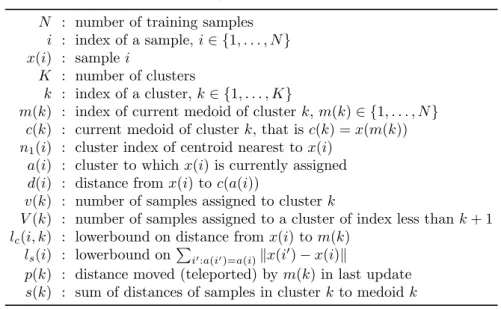
Table 4: Table Of Notation Fortrikmeds
N : number of training samples
i : index of a sample,i∈ {1, . . . , N} x(i) : samplei
K : number of clusters
k : index of a cluster,k∈ {1, . . . , K}
m(k) : index of current medoid of clusterk,m(k)∈ {1, . . . , N} c(k) : current medoid of clusterk, that isc(k) =x(m(k))
n1(i) : cluster index of centroid nearest tox(i) a(i) : cluster to whichx(i) is currently assigned
d(i) : distance fromx(i) toc(a(i))
v(k) : number of samples assigned to clusterk
V(k) : number of samples assigned to a cluster of index less thank+ 1
lc(i, k) : lowerbound on distance fromx(i) tom(k)
ls(i) : lowerbound onP
i0:a(i0)=a(i)kx(i0)−x(i)k
p(k) : distance moved (teleported) bym(k) in last update
s(k) : sum of distances of samples in clusterk to medoidk
Algorithm 10 update-sum-bounds
fork= 1 :K do
// Obtain absolute and net fluxes of energy and count, for clusterk
Jabs s (k) = ∆s−in(k) + ∆s−out(k) Jnet s (k) = ∆s−in(k)−∆s−out(k) Jabs n (k) = ∆n−in(k) + ∆n−out(k) Jnet n (k) = ∆n−in(k)−∆n−out(k) fori=V(k−1) :V(k)−1do
// Update the lower bound on the sum of distances
ls(i)←ls(i)−min(Jabs
s (k)− Jnnet(k)d(i),Jnabs(k)d(i)− Jsnet(k))
end for end for
SM-I
Datasets
• Birch1,Birch2 : Synthetic 2-D datasets available fromhttps://cs.joensuu.fi/sipu/datasets/
• Europe : Border map of Europe available fromhttps://cs.joensuu.fi/sipu/datasets/
• U-Sensor Net : Undirected 2-D graph data. Points drawn uniformly from unit square, with an undirected edge connecting points when the distance between them is less than 1.25√N
• D-Sensor Net : Directed 2-D graph data. Points drawn uniformly from unit square, with directed edge connecting points when the distance between them is less than 1.45√N, direction chosen at random.
• Europe rail : The European rail network, the shapefile is available at http://www.mapcruzin.com/ free-europe-arcgis-maps-shapefiles.htm. We extracted edges from the shapefile usingnetworkx avail-able athttps://networkx.github.io/.
Algorithm 11 contiguate
// This function performs an in place rearrangement over of variablesa, d, l, xandm
// The permutation applied toa, d, l andxhas as result a sorting by cluster, //a(i) =kifi∈ {V(k−1), V(k)}fork∈ {1, . . . , K}
// and moreover that the first element of each cluster is the medoid, //m(k) =V(k−1) fork∈ {1, . . . , K}
• Pennsylvania road The road network of Pennsylvania, the edge list is available directly fromhttps://snap. stanford.edu/data/
• Gnutella Peer-to-peer network data, available fromhttps://snap.stanford.edu/data/
• MNIST (0)The ‘0’s in the MNIST training dataset.
• Conflong The conflongdemo data is available fromhttps://cs.joensuu.fi/sipu/datasets/
• Colormo The colormoments data is available at http://archive.ics.uci.edu/ml/datasets/Corel+ Image+Features
• MNIST50 The MNIST dataset, projected i
![Figure 3: Comparison of TOPRANK and our algorithm trimed on simulated data. On the left, points are drawn uniformly from [0, 1] d for d ∈ {2,](https://thumb-us.123doks.com/thumbv2/123dok_us/739801.2593667/9.892.113.843.107.346/figure-comparison-toprank-algorithm-trimed-simulated-points-uniformly.webp)

![Figure 6: Illustrating the parameters α, β and ρ of Theorem 3.2. Here we draw N = 101 samples uniformly from [−1, 1] and compute their energies, plotted here as the series of points](https://thumb-us.123doks.com/thumbv2/123dok_us/739801.2593667/18.892.224.737.100.322/figure-illustrating-parameters-theorem-samples-uniformly-compute-energies.webp)