Alive SMC
2: Bayesian Model Selection for Low-Count Time
Series Models with Intractable Likelihoods
C. C. Drovandi and R. A. McCutchan Mathematical Sciences
Queensland University of Technology, Brisbane, Australia 4000
email: [email protected]
April 28, 2015
Abstract
In this paper we present a new method for performing Bayesian parameter inference and model choice for low count time series models with intractable likelihoods. The method involves incorporating an alive particle filter within a sequential Monte Carlo (SMC) algorithm to create a novel pseudo-marginal algorithm, which we refer to as alive SMC2. The advantages of this approach over competing approaches is that it is naturally adaptive, it does not involve between-model proposals required in reversible jump Markov chain Monte Carlo and does not rely on potentially rough approximations. The algorithm is demonstrated on Markov process and integer autoregressive moving average models applied to real biological datasets of hospital-acquired pathogen incidence, animal health time series and the cumulative number of prion disease cases in mule deer.
Keywords: Approximate Bayesian computation, INARMA models, evidence, marginal likeli-hood, Markov processes, particle filters, pseudo-marginal methods, sequential Monte Carlo.
1
Introduction
In many biological applications there is significant uncertainty about which model is responsi-ble for the generation of some observed dataset (see, for example, Miller et al. (2006) and Lee et al. (2015)). The data may take the form of a time series consisting of counts of the number of events occurring in discrete or continuous time. Further, such data can be stochastic and thus it is important to model it as such (Bailey, 1964, pp 1). Unfortunately many useful bio-logical stochastic models, such as continuous time Markov processes and discrete time integer autoregressive moving average (INARMA) models, do not possess a computationally feasible (or tractable) likelihood function. However, simulation from such models is often straightfor-ward. For these intractable models, standard approaches to model selection are difficult to apply and/or implement (Marin et al., 2014; Didelot et al., 2011). The purpose of this paper is to present a new approach to perform Bayesian parameter inference and model selection
for a small number of candidate models and demonstrate it on several real datasets in health and infectious diseases.
Our approach falls within the class of pseudo-marginal methods (Andrieu and Roberts, 2009), which perform Bayesian inference using an unbiased and positive likelihood estimator. Here we use the alive particle filter of Jasra et al. (2013); Drovandi et al. (2015). For a fixed value of the model parameter, this particle filter allows matching on observations one-at-a-time. Hence exact matching with low count time series data is possible. When this is not feasible some tolerance can be introduced, resulting in approximate Bayesian inferences (e.g. Beaumont et al. (2002)). We adopt the alive particle filter as presented in Drovandi et al. (2015), which includes auxiliary variables that carry information to allow the sequential simulation of the model. Through these auxiliary variables, a rich set of models and situations can be handled. The novelty of this paper is the inclusion of this alive filter within the sequential Monte Carlo squared (SMC2) algorithm of Chopin et al. (2013) to create a new pseudo-marginal algorithm (alive SMC2) to perform Bayesian parameter inference and model selection for models of low count time series data with intractable likelihoods.
Drovandi et al. (2015) incorporate the alive particle filter within a (reversible jump) Markov chain Monte Carlo (RJMCMC) algorithm and apply it to similar models and applications presented in this paper. However, the approach has several drawbacks. It is well known that it is difficult to devise efficient between-model proposals in RJMCMC (see, for example, Hastie and Green (2012)). In contrast, our method performs SMC individually on each model and uses a well known and simple estimate of the evidence (also known as the marginal likelihood) for a particular model, which is straightforward to calculate from the SMC importance weights (Del Moral et al., 2006). Thus our approach avoids the need for between-model proposals and is appropriate when there are a small number of competing models. Further, MCMC approaches are not naturally parallel algorithms and they have difficulty exploring multi-modal targets. SMC uses a population of parameter values across the parameter space and many of the expensive computations associated with SMC can be done in parallel for each particle. Finally, the approach of Drovandi et al. (2015) requires a reasonable starting value so that it is computationally feasible to estimate the likelihood (based on the full dataset) at this initial value. Our approach uses a population of parameter values and initially requires matching on only the first observation, and thus overcomes this issue to a large extent. For some of the models considered in this paper there are other approaches available in the literature. A general method for models with intractable likelihoods is approximate Bayesian computation (ABC, see Beaumont et al. (2002) for example). ABC estimates the likelihood non-parametrically using model simulations. For ABC to be feasible it is often necessary to reduce the full dataset to a low-dimensional summary statistic, implying a loss of information (see Blum et al. (2013)). In general there is an issue with fully Bayesian model selection when the data have been reduced to a summary statistic (see Marin et al. (2014)). White et al. (2015) and Barthelm´e and Chopin (2014) present fast and potentially summary statistic free ABC methods that allow the matching of observations one-at-a-time. Both approaches offer approximations of the evidence, facilitating approximate Bayesian model choice. However, both of these methods are currently restricted in terms of the types of models that can be considered and involve potentially rough approximations to allow for fast solutions.
reviews the alive particle filter of Drovandi et al. (2015) and provides details of the modifica-tions necessary to include it in the SMC2algorithm. The main novel contribution of the paper, the alive SMC2 algorithm, is presented in Section 2.2. Section 3 illustrates the algorithm on Markov process and INARMA models based on several biological datasets in animal health and infectious diseases. Section 4 concludes the article with a discussion on the limitations of the method and possible avenues for further research.
2
Methodology
We only require notation for a single model as our method is run on models individually. Here we consider complex models of low-count time series data,y1:T, whereT is the number of observations andyt, possibly vector-valued, is the tth observation. In a Bayesian analysis, a prior distribution,p(θ), is required on the model parameter, θ. Of interest is the posterior distribution, p(θ|y1:T), which is proportional to the likelihood function,p(y1:T|θ), times the prior, and has the normalising constant, p(y1:T) = R
θp(y1:T|θ)p(θ)dθ. We refer to this
normalising constant as the evidence. Note that this quantity is often referred to as the marginal likelihood. However, we do not use this term as the definition of the marginal likelihood can be ambiguous especially in the presence of Bayesian models that require latent variables. The evidence is important for Bayesian model choice, as the model with the highest evidence is preferred. For the models we investigate, neither the likelihood up to time t,
p(y1:t|θ), nor the conditional likelihood,p(yt|y1:t−1,θ), can be evaluated cheaply as a function
of θ. In Section 2.1 we present the alive particle filter, which is used for unbiased likelihood estimation. The alive particle filter is then incorporated within an SMC algorithm in Section 2.2 to estimate the posterior distribution,p(θ|y1:T), and the evidence, p(y1:T).
2.1 Alive Particle Filter
For a fixedθ and model, our method relies upon being able to compare simulated data with observed data one-at-a-time. The approach that incorporates data up to t, y1:t, is shown in Algorithm 1. The alive particle filter that incorporates only a single observation, say the
tth (conditional on the fact that it has already incorporated data y1:t−1), is obtained by
performing the final iteration of the loop in Algorithm 1. Both are required in the SMC2 algorithm presented in the next section. Drovandi et al. (2015) extend the alive particle filter of Jasra et al. (2013) to include a vector of auxiliary variables, xt, allowing for sequential
simulation of the model. In this paper we use these auxiliary variables to represent unobserved processes and to create a Markov model from a non-Markov model for the observed data. We also introduce the auxiliary variable,st, which represents the simulated data that is compared
withyt. Thus the filter can handle the situation where it is not computationally practicable to perfectly match the observed data at one or several time points. We define a ‘match’ here when ρ(st,yt) ≤ t where t (tolerance) and ρ (discrepancy function) are both user-chosen. Drovandi et al. (2015) select ρ as the sum of the absolute value of the difference between the components of the simulated and observed data. However, other discrepancy functions may be selected; for example, one that depends on the size of the observed data. In this respect the particle filter has connections with ABC, but it is important to note there is
no summarisation of the data and relative lowt can be achieved since the matching occurs sequentially, increasing the accuracy of ABC. For the applications in this paper we are able to enforce exact matching, i.e. t = 0 for t= 1, . . . , T, but we present the method generally
here and also investigate the use of a non-zero tolerance in one of the applications.
The advantage of the alive particle filter in this setting is that we use negative binomial re-sampling until Nx + 1 (where Nx is the number of particles in the particle filter) matches
are obtained. This helps to ensure that the particle filter does not break down unlike the bootstrap particle filter (Gordon et al., 1993), which may not generate any matches in the binomial matching consisting of Nx trials causing the particle filter to collapse. The
out-put of the alive particle filter is a particle approximation {xjt,sjt}Nx
i=1 of the filtering
dis-tribution p(xt,st|θ,y1:t, 1:t). However, and importantly, the alive filter produces as a
by-product an unbiased estimator of the likelihoodp(y1:t|θ, 1:t) in the context of Algorithm 1
andp(yt|y1:t−1,θ, 1:t) in the context of the final iteration of the loop in Algorithm 1, which we
denote as ˆp(y1:t|θ, 1:t) and ˆp(yt|y1:t−1,θ, 1:t), respectively. It does this by simulating until
there areNx+ 1 matches for each observation and not including the results of the (Nx+ 1)th
match in the particle set (that is, the (Nx+ 1)th particle cannot be resampled). Let ni be the number of simulations required to produceNx+ 1 matches on theith observation. Then the unbiased likelihood estimate is given by ˆp(y1:t|θ, 1:t) =Qti=1Nx/(ni−1), where the
sub-traction of one in the denominator ensures an unbiased estimate (see Jasra et al. (2013)) for a single conditional likelihood component,p(yt|y1:t−1,θ, 1:t). The overall likelihood estimate
represents the product of independent unbiased estimates for each individual conditional like-lihood component. It should be noted that the weight for each particle in the alive particle filter is always the same, so maintenance of the weights is not required.
To ensure that our approach is computationally practicable, we include an intervention in the particle filter that stops the process if too many simulations,ni, are required to produce
Nx+ 1 matches. There may be several reasons why this might occur. Firstly, if the model is mis-specified, simulations from the model are unlikely to match with the data. This calls for more appropriate modelling. Secondly, the model could produce highly variablest. Here it
might be necessary to increase the tolerance for one or more observations. The third reason, which occurred in all the applications in this paper, is when a parameter value is proposed in the extreme tails of the current posterior target att. When the number of simulations exceeds the threshold,K (whereK is set large), we set the (conditional) likelihood to be estimated as 0 for that parameter proposal. This may introduce some error. However, our experience with the method is that this intervention has little impact on the resulting posterior or evidence estimates, since the likelihood of these poor proposals is small relative to otherθsamples that are better supported by the data.
2.2 SMC2 with the Alive Particle Filter 2.2.1 The Algorithm
Here our aim is to obtain an approximation of the posteriorp(θ|y1:T, 1:T) and also the evi-dencep(y1:T|1:T) =
R
θp(y1:T|θ, 1:T)p(θ)dθ. To simplify the notation we setZt=p(y1:t|1:t).
Chopin et al. (2013) present a so-called SMC2 algorithm that can be used to estimate such
Algorithm 1The alive particle filter with auxiliary variables for data y1:t.
Input: A value of the parameter,θ, the number of particles,Nx, the time series data,y1:t, up to time
t, the tolerances,1:t, up to timet, and the maximum number of simulations allowed,K.
Output: Log of the estimated likelihood based on datay1:t, log ˆp(y1:t|θ, 1:t), and a set of particles, {xjt,sjt}Nx
j=1.
1: For notational simplicity set log ˆp(y1:0|θ, 1:0) = 0 2: Obtain initial simulated data, si
0, and auxiliary variable information, x j 0, for j = 1, . . . , Nx if necessary 3: fori= 1tot do 4: Setni= 0 5: fork= 1 toNx+ 1do 6: matched = ‘no’
7: whilematched == ‘no’ do
8: Resample an indexrfrom the set{1, . . . , Nx}with equal weights
9: Generates∗i andx∗i fromp(si,xi|sri−1,x r i−1,θ) 10: Setni =ni+ 1
11: if ni==K then
12: Set ˆp(y1:t|θ, 1:t) = 0 and return 13: end if
14: if ρ(s∗i,yi)≤i then
15: Setsk
i =s∗i,xki =x∗i and matched = ‘yes’ 16: end if
17: end while
18: end for
19: Set log ˆp(yi|y1:i−1,θ, 1:i) = log(nNx i−1)
20: Set log ˆp(y1:i|θ, 1:i) = log ˆp(y1:i−1|θ, 1:i−1) + log ˆp(yi|y1:i−1,θ, 1:i) 21: end for
A particle filter is used to unbiasedly estimate the likelihood increments required and is in-cluded within an overarching SMC algorithm that introduce the data one-at-a-time (i.e. data annealing). The approach of Chopin et al. (2013) is an extension of the more standard SMC algorithm of Chopin (2002) that allows for unbiased estimation of the likelihood. Here we pro-vide a novel approach that incorporates the alive particle filter of Section 2.1 within SMC2 in order to obtain necessary unbiased estimates so that Bayesian posterior inference and evidence estimation can be performed on our models of interest.
SMC works by traversing a set of Nθ particles through a sequence of probability
distribu-tions, starting from one that is easy to sample from (e.g. the prior) and ending at the target (the posterior distribution in Bayesian statistics) by iteratively applying a sequence of re-weighting, re-sampling and mutation steps. Our sequence of target posterior distributions is defined through data annealing. In the SMC algorithm of Chopin (2002), which assumes a computable likelihood, a properly weighted sample, {θit, Wti}Nθ
i=1, from p(θ|y1:t) is produced
at each iteration. To proceed from target t−1 to t in the context of data annealing, the θ samples are re-weighted using the unnormalised weights
wt=Wt−1p(yt|y1:t−1,θ), (1)
which requires evaluation of the conditional likelihood, p(yt|y1:t−1,θ). Unfortunately, this
likelihood is not available for the models we consider. However, we are able to estimate it unbiasedly using the alive particle filter in Algorithm 1 (the final iteration of the for loop). The information iny1:t−1 is summarised through the auxiliary variables xt−1 and st−1, and
for a particular value of θ, our algorithm maintains a collection of samples, {xjt−1,sjt−1}Nx j=1,
from the probability distributionp(xt−1,st−1|θ,y1:t−1,1:t−1). This collection of samples are
provided for Algorithm 1 (final iteration of the for loop in this context) in order to simulate the model forward up to timet. One iteration of the alive particle filter is performed, which involves resampling from {xjt−1,sjt−1}Nx
j=1, simulating forward to time t and noting whether
a match is produced. If a match is not produced, then one returns to the resampling stage. This process is repeated untilNx+ 1 matches have been proposed. Then an unbiased estimate
of p(yt|y1:t−1,θ, 1:t) is given by Nx/(nt−1). Note that if i = 0 for i = 1, . . . , t then the
alive particle filter step produces an unbiased estimate of the actual likelihood increment,
p(yt|y1:t−1,θ). If i >0 is required for any i then the alive particle filter step produces an
unbiased estimate of an approximate likelihood.
The particle set representing the target distribution at timetwe denote as{θit,[{xjt,sjt}Nx j=1]i, Wi
t,pˆ(y1:t|θti, 1:t)}Ni=1θ . For the ith particle, we record the estimate of the likelihood based
on data seen up to the current timet, ˆp(y1:t|θit, 1:t). As mentioned earlier, we also maintain a collection of the auxiliary variables for the ith particle to enable forward simulation. The particle set {θit, Wi
t} Nθ
i=1 represents a weighted sample from the marginal target of interest, p(θ|y1:t, 1:t). As one moves through the sequence of target distributions, the variability in the weights tends to increase, which leads to a reduction in the effective sample size (ESS, see Liu and Chen (1998)). When the ESS falls below some threshold (which we set asNθ/2),
we resample the entire joint particle set according to the weights, Wti, i = 1, . . . , Nθ. The motivation for the resampling step is to duplicate promising particles with relatively high weight and discard those with relatively small weight. The resampling step boosts the ESS back toNθ but results in particle duplication. See Del Moral et al. (2006) for more details.
To enhance diversity, an MCMC kernel can be used with the current target at timetset as the invariant distribution. In an ideal SMC algorithm, the acceptance ratio of the Metropolis-Hastings kernel would involve calculating the likelihood based on all the data seen so far,
p(y1:t|θ). The exact likelihood is unavailable to us, so we call on the alive particle filter in Algorithm 1, which incorporates datay1:t. The MCMC move step requires the specification of a proposal distribution for theθspace,q(·|·). A major advantage of the SMC approach is that a weighted sample from the target is available and can be used to form an efficient proposal distribution. A standard approach is to use the empirical covariance matrix of the particles as the covariance matrix of a multivariate normal random walk proposal (e.g. Drovandi and Pet-titt (2011a); Fearnhead and Taylor (2013)), which we adopt here for simplicity. The drawback of using an MCMC kernel for diversity is that acceptance of the proposal is not guaranteed. Sherlock et al. (2014) suggest an optimal acceptance rate of roughly 7% for pseudo-marginal MCMC. Whilst this optimal acceptance rate may not carry over to when MCMC is used within SMC, some rejection must take place in the MCMC move step. Therefore we repeat the MCMC move stepRtimes on each particle to enhance diversity. Here we keepRconstant, but it is possible to adaptR (see Section 4 for more details).
We refer to our approach as alive SMC2, which is shown in full in Algorithm 2. Our approach inherits the advantages that SMC maintains over MCMC. In particular, because there is a population of particles, SMC is less prone to getting ‘stuck’ as in a single MCMC chain, adaptive and efficient proposal distributions can be easily constructed and there is a possibility that multi-modal posteriors can be represented. A major advantage of SMC over MCMC in the context of Bayesian model choice, is that SMC produces an estimate of the evidence, which can be converted into estimates of posterior model probabilities. We discuss the calculation of the evidence further below. Drovandi et al. (2015) incorporate the alive particle filter within an MCMC algorithm. The method relies on determining an appropriate starting value so that it is possible to ‘match’ the simulated data with the observed data. Since our algorithm necessarily uses an unbiased likelihood estimator, it will be less efficient than an idealised SMC algorithm where exact likelihood calculation is possible. Because the likelihood is estimated, the particle weights will degenerate faster, leading to more resampling and MCMC move steps. Further, the acceptance rate of the MCMC move step of the alive SMC2 will be lower compared to when the exact likelihood is computable. These inefficiencies will be highlighted in practice in Section 3.2. Despite these issues, the empirical results shown in Section 3 demonstrate the usefulness of the alive SMC2 method.
As noted earlier in Section 2.1, if the alive particle filter needs too many simulations to obtain a match with a particular data point for some θ, then the estimated likelihood is set to 0. The re-weighting step of alive SMC2 relies on the conditional likelihood estimate in the final iteration of the for loop in Algorithm 1. When this conditional likelihood estimate is set to 0, the corresponding weight of that particle is set to 0, rendering it useless for the rest of the algorithm. This is why a weight check is included in line 7 of Algorithm 2. The MCMC move step of alive SMC2 relies on Algorithm 1. When the likelihood estimate is set to 0, the proposed parameter is rejected with certainty.
As mentioned earlier, SMC produces a convenient estimate of the evidence,p(y1:T), which we denote here asZT for simplicity. The estimate is based on the identityZTc =
QT
t=1Zt/Zt\−1.
Algorithm 2Alive SMC2 algorithm.
Input: Number ofθ samples,Nθ, the number of particles for the alive particle filter,Nx, number of
MCMC repeats,R, the data,y1:T, and the tolerances,1:T.
Output: Collection of{θi, Wi}Nθ
i=1samples fromp(θ|y1:T, 1:T) and estimates of the ratios of
normal-ising constants,Z\t/Zt−1, fort= 1, . . . , T withZ0= 1.
1: Generate samples from the prior distribution,θi0∼p(θ) fori= 1, . . . , Nθ 2: Initialise weightsWi
0 = 1/Nθ fori= 1, . . . , Nθ
3: Form initial collection of auxiliary variables [{xj0,sj0}Nx j=1]
i fori= 1, . . . , N
θ if required. 4: The initial collection of particles is given by{θi0,[{x
j 0,s j 0} Nx j=1] i, Wi 0} Nθ i=1 5: fort= 1to T do 6: fori= 1to Nθdo 7: if Wi t−16= 0then
8: Run the last iteration of the for loop of the alive particle filter of Algorithm 1 using [{xjt−1,sjt−1}Nx j=1] i as input to estimate ˆp(y t|y1:t−1,θ i t−1, 1:t) and obtain [{x j t,s j t} Nx j=1] i 9: end if 10: end for 11: Setθit=θit−1 fori= 1, . . . , Nθ 12: Update unnormalised weightswi
t=Wti−1pˆ(yt|y1:t−1,θ i
t, 1:t) fori= 1, . . . , Nθ 13: Estimate ratio of normalising constantsZ\t/Zt−1=P
Nθ i=1w
i t 14: Update likelihood estimate ˆp(y1:t|θit, 1:t) = ˆp(y1:t−1|θ
i
t, 1:t−1)ˆp(yt|y1:t−1,θ i
t, 1:t) for i =
1, . . . , Nθ
15: Normalise the weights Wti=wti/
PNθ k=1w k t fori= 1, . . . , Nθ 16: Compute ESS = 1/PNθ i=1(W i t)2 17: if ESS< Nθ/2then
18: Sample an indexrifrom the discrete set{1, . . . , Nθ}with probabilities{Wti} Nθ i=1with replace-ment fori= 1, . . . , Nθ 19: Set (θit,[{xjt,si t} Nx j=1]i,pˆ(y1:t|θ i t)) = (θ ri t ,[{x j t,s j t} Nx j=1]ri,pˆ(y1:t|θ ri t )) fori= 1, . . . , Nθ 20: SetWi t = 1/Nθfori= 1, . . . , Nθ
21: fori= 1, . . . , Nθ (and repeat this loopRtimes)do 22: Proposeθ∗∼q(·|θit)
23: Run the alive particle filter of Algorithm 1 to obtain ˆp(y1:t|θ∗, 1:t) and [{xjt,s j t} Nx j=1]∗ 24: Computeα= min1,pˆ(y1:t|θ ∗, 1:t)p(θ∗)q(θit|θ ∗) ˆ p(y1:t|θit,1:t)p(θit)q(θ∗|θit) 25: if U(0,1)< αthen 26: Set (θit,[{xjt,sjt}Nx j=1]i,pˆ(y1:t|θ i t, 1:t)) = (θ∗,[{xjt,s j t} Nx j=1]∗,pˆ(y1:t|θ ∗, 1:t)) 27: end if 28: end for 29: end if 30: end for
summing the unnormalised importance weights (see equation (1)),Z\t/Zt−1 =PN
i=1wit. Once
the evidence has been estimated for each postulated model, it is straightforward to convert these into estimates of the posterior model probabilities. The evidence estimator still applies even if the likelihood increments are unbiasedly estimated (see, for example, Chopin et al. (2013)). If all of the tolerances, t fort= 1, . . . , T, are set to zero, the alive SMC2 approach provides a direct approximation of what would have been obtained with an ideal SMC algo-rithm (see Section 3.2 for some empirical results) whereas if any of the tolerances are non-zero then our method produces an estimate of an approximate evidence. Our method does not involve any data reduction, thereby avoiding the problem that Bayes factors based on a set of summary statistics are not consistent estimators of Bayes factors based on the full data (see Marin et al. (2014) for example).
The SMC estimator of the evidence may suffer from too much Monte Carlo variability to be able to precisely discriminate between models. Here we describe an alternative approach that can be used based on the output of the parameter posterior distribution estimates from alive SMC2 (see also Drovandi et al. (2015)). This approach could be suitable for the relatively low dimensional models that we consider here. First we fit a parametric distribution, with densitygφ(θ) and parameterφ, to the parameter posterior distribution for a particular model based on the weighted sample, {WTi,θiT}Nθ
i=1. This amounts to estimating the parameter φ
from the posterior samples to produce ˆφ, which can be done using maximum likelihood, for example. Then, gφˆ(θ) forms a density that can be used to develop a simple unbiased
importance sampling (IS) estimator of the evidence given by
ˆ p(y1:T|1:T) = 1 B B X i=1 ˆ p(y1:T|θi, 1:T)p(θi) gφˆ(θi) , (2) whereθi iid
∼ gφˆ(θ) for i= 1, . . . , B. To avoid high variance IS estimators, it is necessary for
the tails of g to cover those of the target, p(θ|y1:T, 1:T). This can be achieved by making
some modifications to ˆφ, for example, inflating variance parameters.
2.2.2 Highly informative first observation
When a relatively vague prior distribution is used it is possible that the first observation is highly informative relative to that prior, which could lead to a large reduction in the ESS. We provide an alternative implementation that can be used for the first observation for this scenario. This involves repeated simulations from the prior distribution until Nθ
parameter values have simulated data that match the first observation. The alive particle filter is then run for these Nθ parameter values in order to estimate the likelihood and
to generate the auxiliary variables at t = 1. The output of this procedure is given by
{θi1,[{xj1,sj1}Nx
j=1]i, W1i,pˆ(y1|θi1, 1)} Nθ
i=1 and an estimate of the ratio of normalising constants, \
Z1/Z0 with Z0 = 1. We also have thatW1i = 1/Nθ fori= 1, . . . , Nθ. Once this procedure is complete then one moves to line 5 of Algorithm 2 where the loop starts fromt= 2. Further details are provided in Appendix A.
3
Examples
This section consists of several examples of differing complexity. The first example involving a continuous time Markov model for the transmission of a pathogen within a hospital ward is used to validate the approach as the exact likelihood can be computed. Here we compare two different transmission models. Section 3.2 considers the analysis of several animal health time series datasets using four INARMA models, with zero-inflated Poisson innovations to account for the overdispersion in the data. Finally, in Section 3.3, an intractable Markov process model is considered for the transmission of chronic wasting disease in mule deer. Here we consider two different transmission models. Throughout all examples we use Nθ = 1000, Nx= 50,K = 100000 andR= 10 for the alive SMC2 algorithm. The values ofNx andR are chosen to produce a reasonably diverse set of particles representing the target distributions throughout the algorithm. The value of Nθ controls the number of particles representing
the parameter posterior distributions. The value of K is conservatively set to be very large. Throughout all examples we assume that the candidate models are equally likely a priori.
3.1 Nosocomial Pathogen Transmission
This example serves as an illustration of the method as it is possible to calculate the likelihood using the approach of Drovandi and Pettitt (2008). Drovandi and Pettitt (2008) consider a stochastic model for the spread of Methicillin-resistantStaphylococcus aureus(MRSA) within a hospital ward. In the model, colonisation of MRSA in patients is facilitated by health-care workers through possible lack of hand hygiene. The model has colonised patient,Yp(t), and
colonised health-care worker,Yh(t), populations and assumes a constant ward size of M, for both patients and health-care workers. The data consists of the number of new colonisa-tion cases per week (weekly incidence) within the ward, which can be routinely collected by hospitals. These data for a 184 week period at the Princess Alexandra Hospital, Brisbane, Australia are shown in Drovandi et al. (2015). A counter variable, N(t), is included in the model of Drovandi and Pettitt (2008) that represents the incidence.
McBryde et al. (2007) and Drovandi and Pettitt (2008) apply a so-called pseudo-equilibrium approximation where the mean of the colonised health-care worker population is considered and the rate of change of this population is set to 0. This provides an equation that de-terministically relates the discrete colonised patient variable to the now-continuous colonised health-care population (denoted ¯Yh(t)), which simplifies the model. Drovandi and Pettitt
(2011b) demonstrate that this provides a good approximation in the context of a Bayesian analysis on the same data analysed here. This approximation eliminates theYh(t) population
from the model. The possible transitions in the model are described in Lee et al. (2015). Two different transmission models are considered by Lee et al. (2015). The first is referred to here as the Standard model and uses a standard mass action assumption thatf( ¯Yh) =φsY¯h
and the second, referred to here as the Greenwood model, uses the assumption of Greenwood (1931) whereby provided that at least one person is colonised, there is a constant colonisation pressure for the corresponding susceptible group so that f( ¯Yh) = φg1( ¯Yh > 0). We use the
priors φs ∼ U(0,0.5) and φg ∼ U(0,0.5) (see Web Appendix B of Lee et al. (2015) for a justification). The pseudo-equilibrium expressions for ¯Yh(t) for the Standard and Greenwood
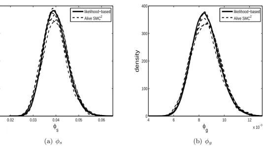
0.02 0.03 0.04 0.05 0.06 0 20 40 60 80 φs density likelihood−based Alive SMC2 (a) φs 4 6 8 10 12 x 10−3 0 100 200 300 400 φg density likelihood−based Alive SMC2 (b)φg
Figure 1: Posterior distributions for the parametersφsandφgof the Standard and Greenwood
models, respectively, for the MRSA example. The dashed lines are results from 5 independent runs of alive SMC2 and the solid line is based on a long run of MCMC using the exact likelihood.
This example is useful for validation purposes as the likelihood can be calculated using the approach of Drovandi and Pettitt (2008) (see Drovandi et al. (2015) for further details). For our approach, the number of colonised patients is unobserved throughout the process, thus we setxt =Yp(t). The data correspond to yt =N(t). We find that the first observation is
highly informative relative to the priors specified, so we use the implementation in Section 2.2.2. To assess the MC variability of alive SMC2, we repeat the algorithm 10 times. The posterior distributions obtained from the alive SMC2 method are shown in Figure 1 for 5 of the runs. It is evident that there is close agreement with the likelihood-based approach. To two decimal places, the posterior model probability of the Standard model obtained from alive SMC2 (averaged over the 10 runs) is 0.96 (with a MC standard error of about 0.01), which is consistent with 0.97 obtained with the likelihood-based approach.
3.2 Animal Health Time Series Datasets
The integer autoregressive moving average (INARMA) model is the discrete version of the pop-ular ARMA model for stationary Gaussian time series (Box et al., 1994). The INARMA(p, q) model is given by Yt= p X i=1 αi◦Yt−i+ut+ q X j=1 βj◦ut−j,
where◦ is the binomial thinning operator (that is, if W =α◦Y, then W ∼Binomial(Y, α)) and ut for t ∈ N is a sequence of independent and identically distributed discrete random
variables. A popular choice isut iid
by Jazi et al. (2012) who propose to use a zero-inflated Poisson (ZIP) model,ut iid
∼ZIP(λ, ρ), whereρ∈(0,1) is a probability that provides a second mechanism forutbeing 0, for datasets that exhibit over-dispersion. We refer to this as the ZIP INARMA model. The likelihood is cumbersome for all ZIP INARMA models bar the ZIP INAR(1) model, which involves the convolution of a binomial and a ZIP random variable.
The ZIP INAR models are Markovian and do not require any auxiliary information in the alive particle filter. However, the ZIP INMA and ZIP INARMA models are non-Markovian due to the moving average component. However, for a single moving average component, sequential simulation of the model is facilitated by introducing the auxiliary variablext=ut
into the alive SMC2 algorithm. Higher order moving average models could be considered by introducing more auxiliary information.
We apply our method to data provided by the Ministry for Primary Industries, New Zealand, and consists of animal health laboratory datasets. The recorded data is the monthly number of submissions of bovine displaying certain symptoms to animal health laboratories, in 2003-2009 for a total of 84 observations, for a region in New Zealand. Here we consider the time series relating to symptoms abortion, anorexia, illthrift, skin lesions and sudden death. We find that for these data the zero-inflation is required for a good fit. Here we compare ZIP INAR(1), ZIP INAR(2), ZIP INMA(1) and ZIP INARMA(1,1) models for each dataset. Note that the frequentist approach of Jazi et al. (2012) considers only INAR(1) type models. For simplicity we fixY−1= 0 andY0 = 0, which are required in the ZIP INAR models. The prior
on allαi and βj parameters is set as U(0,1) while we assume that λ∼Exp(1).
Prior to analysing the animal health data, we perform a simulation study. In turn, we allow each of the four models to be the true model and a dataset of T = 200 is simulated from the relevant model and the alive SMC2 algorithm is applied to estimate the posterior model probabilities and the parameter posterior distributions. Three datasets are generated from each model resulting in a total of 12 datasets. More details and results of the simulation study are presented in Appendix B. In short, our algorithm is able to recover the correct model (based on the model with the highest probability) for 11 out of the 12 datasets. When either the ZIP INAR(1) or the ZIP INMA(1) is the true model, it is sometimes confused with the ZIP INARMA(1,1) model. It is evident that the parameter posterior distributions of the true model recover the corresponding true parameter well.
For the ZIP INAR(1) model, the exact likelihood is available. Here we run standard SMC with the exact same implementation as alive SMC2, but with the true likelihood. For when the ZIP INAR(1) is the true model, Appendix B demonstrates agreement between the parameter posterior distributions when using the exact and approximate likelihoods. The appendix also highlights the inefficiency of alive SMC2 relative to ideal SMC but shows an agreement between the evidence estimates when using the unbiased or exact likelihoods.
The posterior model probabilities obtained when applying alive SMC2to the real data is shown in Table 1, which are based on 10 repeated runs of the algorithm. For the skin and illthrift datasets the ZIP INAR(2) model has the most support while the ZIP INARMA(1,1) model is preferred for the sudden death data. The ZIP INAR(2) model seems to have the highest posterior probability for the abort and anorexia datasets but too much MC variability prevents the precise identification of the preferred model. Here we consider the alternative IS estimator as presented in equation (2). For the IS density,g, we use a multivariate normal distribution
Table 1: Posterior model probability results when applying alive SMC2 to the animal health data. For the abort and anorexia datasets, results are also provided for the alternative IS estimator. Shown are the mean posterior model probability for each of the models with the Monte Carlo standard error in parentheses, estimated from 10 independent runs of the method. Shown in bold is the preferred model for each dataset.
data method INAR(1) INAR(2) INMA(1) INARMA(1,1)
abort alive SMC2 0.35 (0.06) 0.45 (0.08) 0.014 (0.003) 0.18 (0.05) abort IS 0.34 (0.01) 0.51 (0.02) 0.013 (0.002) 0.14 (0.01) anorexia alive SMC2 0.29 (0.05) 0.43 (0.07) 0.016 (0.002) 0.27 (0.05) anorexia IS 0.31 (0.02) 0.47 (0.02) 0.014 (0.001) 0.20 (0.01) illthrift alive SMC2 0.23 (0.04) 0.52 (0.08) 0.00 (0.00) 0.25 (0.06) skin alive SMC2 0.17 (0.03) 0.68 (0.04) 0.09 (0.02) 0.05 (0.006) sudden alive SMC2 0.21 (0.05) 0.09 (0.02) 0.01 (0.002) 0.69 (0.06)
with the empirical covariance matrix inflated by a factor of 2. The results obtained from performing 1000 IS iterations on each model and repeating the process 10 times for the abort and anorexia datasets are also shown in Table 1. Through these extra computations, and utilising the output of alive SMC2, we are able to more definitively identify the ZIP INAR(2) model as the preferred model. In Appendix C, we show the parameter posteriors for the model with the highest posterior model probability for each dataset. It is important to note that the estimation approach of Jazi et al. (2012) considers only INAR(1) type models. These datasets illustrate that more complex models are warranted and that there can be substantial model uncertainty, which can be quantified using alive SMC2.
3.3 Chronic Wasting Disease in Mule Deer
Finally, we consider a dataset on chronic wasting disease (CWD) in captive mule deer held at the Foothills Wildlife Research Facility, Colorado Division of Wildlife (see Miller et al. (2006)). This dataset consists of the cumulative number of deaths of mule deer due to CWD observed at various times for two separate epidemics, one from 1974 to 1985 and the second based on a new deer herd from 1992 to 2001. These two datasets can be treated as indepen-dent. Miller et al. (2006) consider several deterministic models to explain the transmission dynamics of CWD for the deer. However, data involving small populations are inherently stochastic. Libo et al. (2014) compare different transmission models as well as formulating these within a deterministic framework (differential equations) and a stochastic framework (stochastic differential equations and Markov jump processes). Since the data are discrete counts, the most appropriate modelling approach is a Markov jump process, whereas stochas-tic and determinisstochas-tic differential equations may be seen as approximations to the Markov jump process. Libo et al. (2014) apply ABC and use a discrepancy function that includes the full datasets, and thus do not generate exact matches of simulated and observed data (or necessarily very close over the full trajectory) as we do here.
Denote the number of (unobserved) susceptible and infected animals at time t as S(t) and
I(t), respectively. Further, denoteC(t) as the cumulative number of deer deaths due to CWD up until time t. Libo et al. (2014) assume the observed data is an undercount of C(t) and
use a binomial observation model. For illustration purposes, we assume that the data are observed without error so that C(t) corresponds to the data observed at some discrete time points. Initially we consider the Markov process formulation of the direct transmission process of Miller et al. (2006). Given the current values of the states,S(t) =i,I(t) =jand C(t) =k, and a small time interval ∆t, the probabilities of various combinations of the states at time t+ ∆t are given by P(S=i+ 1, I =j, C=k) =a∆t+o(∆t), P(S=i−1, I =j, C=k) =mi∆t+o(∆t), P(S=i−1, I =j+ 1, C=k) =βij∆t+o(∆t), P(S=i, I =j−1, C=k) =mj∆t+o(∆t), P(S=i, I =j−1, C=k+ 1) =µj∆t+o(∆t), (3)
whereais the number of deer added annually,mis the per-capita per year natural death rate,
β is the transmission rate per year and µis the per-capita death rate per year due to CWD. The dataset includes the number of deer added to the population each year, so we fix a at those values. Further, the dataset includes an estimate for the natural deer death rate per year and we setm at those values. Note that this is an approximation as the model will not simulate exactly the number of deer added annually and the number of natural deaths per year as what is present in the data. However, it is a reasonable approximation and reduces the number of parameters that need to be estimated. The initial number of susceptible and infective deer at timet= 0, S0l and I0l, are unobserved for the l= 1,2 time periods and are treated as discrete model parameters.
Here we compare the direct transmission model with a model that allows for a latent period where infected animals are not infectious. The model includes an additional variable, L(t), describing the number of deer in the latent phase at timet. It also has an additional parameter that requires estimation, 0< α < 1, which is the proportion of the clinical course spent in latency. The transition probabilities of this model are provided in Appendix D. As in Miller et al. (2006), we assume that L(0) = 0 for both epidemics. The parameter θ for the direct model is thus θ = (β, µ, S01:2, I01:2) and is θ = (β, µ, α, S01:2, I01:2) for the latent model. For the parameters β, µ, S1:2
0 , I01:2 of both models we use the same prior distributions as in Libo
et al. (2014), which were obtained from expert opinion. The priors on eachβ, µ, S0 and I0
parameter are Beta(2,10), Beta(2,5), Discrete U(10,50) and Discrete U(0,20), respectively. We allocate aU(0,1) prior to the parameterα of the latent model.
Since S(t), I(t) andL(t) are unobserved, we have xt = (S(t), I(t)) for the direct model and
xt= (S(t), I(t), L(t)) for the latent model. Hereytcorresponds toC(t). In this example, the
parameterθ grows in dimension as the second epidemic data is introduced. For both models, the first epidemic data is not informative about (S02, I02). Thus, after the first epidemic data has been incorporated, the space is extended by sampling the second epidemic initial condition parameters from their priors. During the incorporation of the second epidemic data, the MCMC move part of the algorithm must incorporate all data from the first epidemic and the relevant data from the second epidemic. We also use the alternative implementation in Section 2.2.2 as we find that the first observation is rather informative.
Here we run alive SMC2 10 times independently on both models. We find that the estimated posterior model probability of the latent model is 0.74 (0.03). We note that this result is in
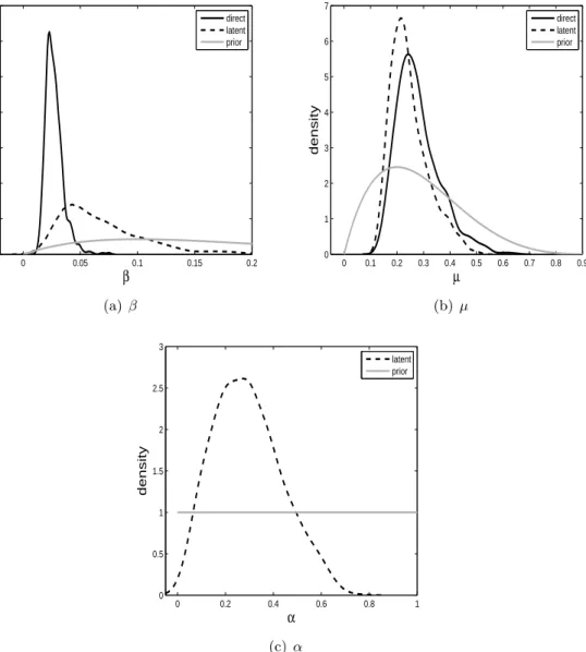
0 0.05 0.1 0.15 0.2 0 10 20 30 40 50 60 70 β density direct latent prior (a)β 0 0.1 0.2 0.3 0.4 0.5 0.6 0.7 0.8 0.9 0 1 2 3 4 5 6 7 µ density direct latent prior (b) µ 0 0.2 0.4 0.6 0.8 1 0 0.5 1 1.5 2 2.5 3 α density latent prior (c) α
Figure 2: Posterior distributions for the parameters of the direct (solid) and latent (dashed) models withβ parameters in (a), µ parameters in (b) and α in (c). The prior distributions are shown in grey.
contrast to Miller et al. (2006), who find preference for the direct model over the latent model. Miller et al. (2006) apply the deterministic formulation of the models we consider here and use the Akaike Information Criterion for model comparison. The posterior distributions of the parameters of the two models from a single alive SMC2 run is shown in Figure 2.
Finally we run alive SMC2 with ρ(st, yt) = |st −yt| (as the data are scalar) and t = 1,
t = 1, . . . , T, to examine the impact of non-exact matching in this application. We obtain general agreement with the exact matching results. The estimated posterior model probability of the latent model is 0.77 (0.02). Appendix E demonstrates that the parameter posterior dis-tributions are similar despite the inexact matching. Further, introducing the inexact matching roughly halved the run times of alive SMC2.
4
Discussion
This article illustrates a new algorithm called alive SMC2 to perform Bayesian parameter inference and model choice on low-count time series models such as Markov processes and INARMA models, which can have computationally intractable likelihood functions. Our approach is preferable to Drovandi et al. (2015) in some aspects as it avoids between-model proposals, mitigates the starting value issue of Drovandi et al. (2015), and it also inherits the advantages that SMC has over MCMC. Unlike Barthelm´e and Chopin (2014) and White et al. (2015), our approach can handle partially observed processes and non-Markov models, and does not rely on potentially crude approximations.
Despite the success of the algorithm demonstrated on several real datasets in this paper, the approach has some limitations. Firstly, SMC struggles in the presence of highly informative observations (Del Moral and Murray, 2014), which can result in very large reductions in the ESS. This can often happen for the first observation when a vague prior distribution is used. We propose a strategy to accommodate the first observation, but unfortunately any particular observation may be highly informative, which could result in an ESS too small to recover from. Because this method falls within the pseudo-marginal framework, it does not scale efficiently to an increase in size of the dataset. Generally speaking, for fixedNx and θ, the variance of the likelihood estimator grows withT (C´erou et al., 2011), resulting in a less efficient algorithm. We discuss this point further below.
An extension of the algorithm would adapt the value ofNxthroughout the algorithm. Initially, when t is small, only a relatively small value of Nx would be required to obtain a precise
estimate of p(y1:t|θ, 1:t). As the data size increases, it becomes more difficult to estimate
the likelihood with low variance, which leads to faster reductions in the ESS. Furthermore, the MCMC move step may suffer from low acceptance probabilities due to overestimation of the likelihood for the data up until timet for larget. Chopin et al. (2013) propose to double the value ofNx each time the MCMC acceptance rate falls below some threshold. This idea could be implemented in our algorithm. Doucet et al. (2015) show that for good performance of pseudo-marginal algorithms, the log-likelihood (at some representative parameter value) should be estimated with a standard deviation of approximately one. It may be possible to estimate the variability using the collection ofθ samples and likelihood estimates for someθ with high posterior support in our algorithm. We could use this to adapt the value of Nx.
Drovandi and Pettitt (2011a), who adapt the value ofRbased on the overall acceptance rate of the previous MCMC move step. We leave these possible extensions for future research.
Acknowledgements
We are grateful to Michael W. Miller and the Colorado Division of Parks and Wildlife for providing access to the prion transmission data. We thank the Surveillance and Incursion Investigation Team, Ministry for Primary Industries, New Zealand, for providing the data on animal health laboratory submissions. The first author would like to thank Tony Pettitt for his comments on an earlier draft.
References
Andrieu, C. and Roberts, G. O. (2009). The pseudo-marginal approach for efficient Monte Carlo computations. The Annals of Statistics, 37(2):697–725.
Bailey, N. T. J. (1964). The elements of Stochastic Processes: with applications to the natural sciences. Wiley, New York.
Barthelm´e, S. and Chopin, N. (2014). Expectation propagation for likelihood-free inference.
Journal of the American Statistical Association, 109(505):315–333.
Beaumont, M. A., Zhang, W., and Balding, D. J. (2002). Approximate Bayesian computation in population genetics. Genetics, 162(4):2025–2035.
Blum, M. G. B., Nunes, M. A., Prangle, D., and Sisson, S. A. (2013). A comparative review of dimension reduction methods in approximate Bayesian computation. Statistical Science, 28:189–208.
Box, G., Jenkins, G. M., and Reinsel, G. C. (1994). Time Series Analysis: Forecasting & Control, 3rd edition. Pearson Education India.
C´erou, F., Del Moral, P., and Guyader, A. (2011). A nonasymptotic theorem for unnormal-ized Feynman–Kac particle models. Annales de l’Institut Henri Poincar´e, Probabilit´es et Statistiques, 47(3):629–649.
Chopin, N. (2002). A sequential particle filter method for static models. Biometrika, 89(3):539–551.
Chopin, N., Jacob, P. E., and Papaspiliopoulos, O. (2013). SMC2: an efficient algorithm for sequential analysis of state space models. Journal of the Royal Statistical Society: Series B (Statistical Methodology), 75(3):397–426.
Del Moral, P., Doucet, A., and Jasra, A. (2006). Sequential Monte Carlo samplers. Journal of the Royal Statistical Society: Series B (Statistical Methodology), 68(3):411–436.
Del Moral, P. and Murray, L. M. (2014). Sequential Monte Carlo with highly informative observations. arXiv:1405.4081v1.
Didelot, X., Everitt, R. G., Johansen, A. M., and Lawson, D. J. (2011). Likelihood-free estimation of model evidence. Bayesian Analysis, 6(1):49–76.
Doucet, A., Pitt, M., Deligiannidis, G., and Kohn, R. (2015). Efficient implementation of Markov chain Monte Carlo when using an unbiased likelihood estimator. To appear in Biometrika.
Drovandi, C. C. and Pettitt, A. N. (2008). Multivariate Markov process models for the transmission of Methicillin-resistantStaphylococcus aureus in a hospital ward. Biometrics, 64(3):851–859.
Drovandi, C. C. and Pettitt, A. N. (2011a). Estimation of parameters for macroparasite population evolution using approximate Bayesian computation. Biometrics, 67(1):225–233. Drovandi, C. C. and Pettitt, A. N. (2011b). Using approximate Bayesian computation to esti-mate transmission rates of nosocomial pathogens. Statistical Communications in Infectious Diseases, 3(1):2.
Drovandi, C. C., Pettitt, A. N., and McCutchan, R. (2015). Exact and approximate Bayesian inference for low count time series models with intractable likelihoods. To appear in Bayesian Analysis.
Fearnhead, P. and Taylor, B. M. (2013). An adaptive sequential Monte Carlo sampler.
Bayesian Analysis, 8(2):411–438.
Gordon, N. J., Salmond, D. J., and Smith, A. F. M. (1993). Novel approach to nonlinear/non-Gaussian Bayesian state estimation. In Radar and Signal Processing, IEE Proceedings F, volume 140, pages 107–113.
Greenwood, M. (1931). On the statistical measure of infectiousness. The Journal of Hygiene, (3):336–351.
Hastie, D. I. and Green, P. J. (2012). Model choice using reversible jump Markov chain Monte Carlo. Statistica Neerlandica, 66(3):309–338.
Jasra, A., Lee, A., Yau, C., and Zhang, X. (2013). The alive particle filter.
http://arxiv.org/abs/1304.0151.
Jazi, M. A., Jones, G., and Lai, C.-D. (2012). First-order integer valued AR processes with zero inflated Poisson innovations. Journal of Time Series Analysis, 33(6):954–963.
Lee, X. J., Drovandi, C. C., and Pettitt, A. N. (2015). Model choice problems using ap-proximate Bayesian computation with applications to pathogen transmission data sets.
Biometrics, 71(1):198–207.
Libo, S., Lee, C., and Hoeting, J. (2014). Parameter inference and model selection in deter-ministic and stochastic dynamical models via approximate Bayesian computation: modeling a wildlife epidemic. http://arxiv.org/pdf/1409.7715.pdf.
Liu, J. S. and Chen, R. (1998). Sequential Monte Carlo methods for dynamic systems.Journal of the American Statistical Association, 93(443):1032–1044.
Marin, J.-M., Pillai, N. S., Robert, C. P., and Rousseau, J. (2014). Relevant statistics for Bayesian model choice. Journal of the Royal Statistical Society: Series B (Statisti-cal Methodology), 76(5):833–859.
McBryde, E. S., Pettitt, A. N., and McElwain, D. L. S. (2007). A stochastic mathematical model of Methicillin-resistantStaphylococcus aureustransmission in an intensive care unit: predicting the impact of interventions. Journal of Theoretical Biology, 245(3):470–481. Miller, W. W., Hobbs, N. T., and Tavener, S. J. (2006). Dynamics of prion disease transmission
in mule deer. Ecological Applications, 16(6):2208–2214.
Sherlock, C., Thiery, A. H., Roberts, G. O., and Rosenthal, J. S. (2014). On the efficiency of pseudo-marginal random walk Metropolis algorithms. arXiv:1309.7209v3.
White, S. R., Kypraios, T., and Preston, S. P. (2015). Piecewise approximate Bayesian com-putation: fast inference for discretely observed Markov models using a factorised posterior distribution. Statistics and Computing, 25(2):289–301.
Appendix A
This appendix contains more details about the method to handle a highly informative first observation in Section 2.2.2 of the main paper. The approach shown in Algorithm 3 replaces lines 1-4 in Algorithm 2 and then in line 5 of Algorithm 2 the loop starts fromt= 2.
Algorithm 3Incorporating the first observation in the alive SMC2 algorithm when the first observation is highly informative.
Input: Number ofθ samples,Nθ, the number of particles for the alive particle filter,Nx, the
first observation, y1, and the tolerance, 1. Output: Collection of particles{θi1,[{xj1,sj1}Nx
j=1]i, W1i,pˆ(y1|θi, 1)} Nθ
i=1and an estimate of the
ratio of normalising constants,Z1/Z0\, with Z0= 1.
1: Set sims = 0
2: for i= 1, . . . , Nθ do
3: whilematched == ‘no’ do
4: Obtain initial auxiliary variables if required, x∗0,s∗0 5: Simulate θ∗∼p(θ)
6: Generates∗1 andx∗1 fromp(s1,x1|s∗0,x∗0,θ
∗ ) 7: Set sims = sims + 1
8: if ρ(s∗1,y1)≤1 then
9: Set θi1 =θ∗ 10: end if
11: end while 12: SetW1i= 1/Nθ
13: Run the alive particle filter of Algorithm 1 with y1 as input to estimate ˆp(y1|θi1, 1)
and obtain [{xj1,sj1}Nx j=1]i
14: end for
15: Set Z1/Z0\ =Nθ/sims
16: Proceed from line 5 in Algorithm 2 but the loop starts from t= 2.
Appendix B
Here we describe the details of the simulation study for the ZIP INARMA models studied in Section 3.2 of the main paper. Four models are considered: ZIP INAR(1), ZIP INAR(2), ZIP INMA(1) and ZIP INARMA(1,1). Each model has a turn at being the true model. For the ZIP INAR(1) model, we useα1 = 0.4, λ= 2 and ρ = 0.7. For the ZIP INAR(2) model, we
use α1 = 0.2, α2 = 0.4, λ= 2 and ρ = 0.7. For the ZIP INMA(1) model, we useβ1 = 0.4,
λ= 2 and ρ = 0.7. Finally, for the ZIP INARMA(1,1) model, we use α1 = 0.4, β1 = 0.4,
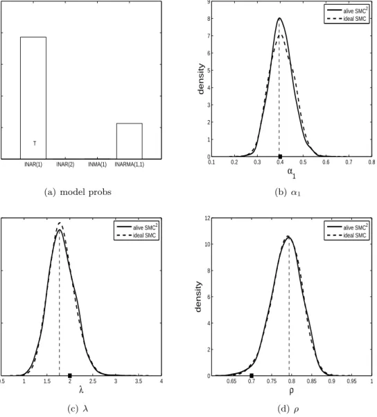
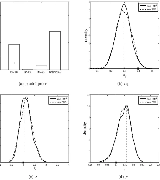
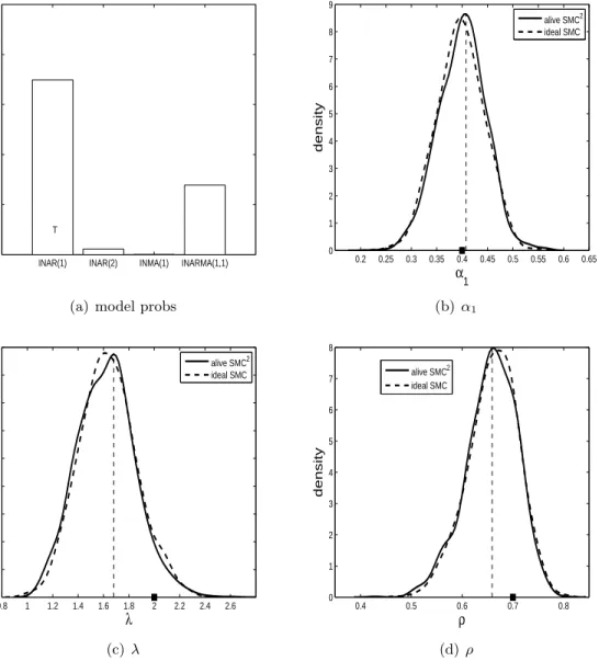
λ= 2 andρ= 0.7. For each model/parameter configuration we simulate three datasets. In subfigure (a) of Figures 3-14 the estimated posterior probabilities of all four models are shown. In these subfigures ‘T’ represents the model that generated the data. It is hoped that the model with the ‘T’ has the highest posterior probability. The other subfigures in Figures 3-14 show the parameter posterior distributions produced by alive SMC2 when the
true model is applied. The square on the x-axis of each subfigure shows the true parameter used to generate the data. The vertical dashed line in each subfigure represents an estimate of the marginal posterior model for the corresponding parameter. Figures 3-5 also show the parameter posterior distributions for when ideal SMC is applied (i.e. SMC with the actual likelihood).
The results for when the ZIP INAR(1) model is true are shown in Figures 3, 4 and 5. For two out of the three datasets, the ZIP INAR(1) model is recovered as the model with the highest probability. It is evident from subfigure (a) in the three figures that the ZIP INAR(1) model can be confused with the ZIP INARMA(1,1) model. The parameter posterior distributions indicate that the true parameter configuration is being recovered well generally.
The results for when the ZIP INAR(2) model is true are shown in Figures 6, 7 and 8. For all three datasets the ZIP INAR(2) model has a posterior model probability close to one, indicating that it is easier to identify this model. The parameter posterior distributions indicate that the true parameter configuration is being recovered well generally.
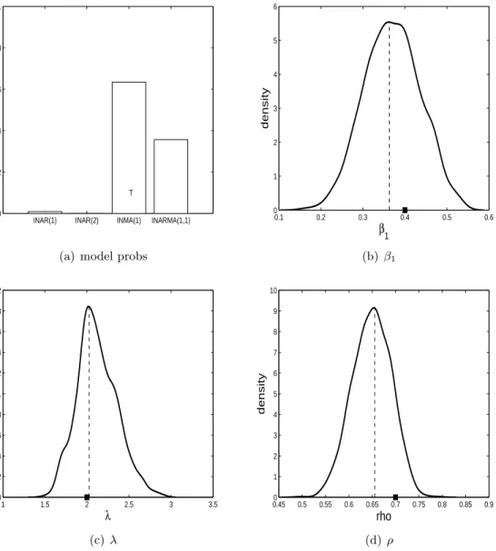
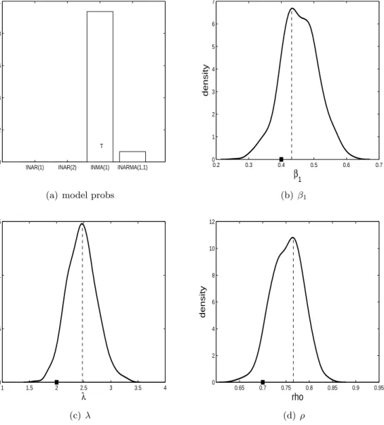
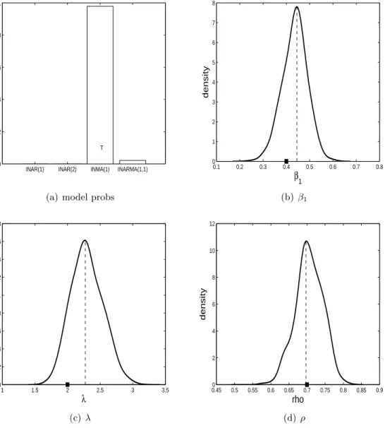
The results for when the ZIP INMA(1) model is true are shown in Figures 9, 10 and 11. For all three datasets, the ZIP INMA(1) model has the highest posterior model probability. However, from the subfigure (a) in the three figures it is evident that the ZIP INMA(1) may be confused with the ZIP INARMA(1,1) model. The parameter posterior distributions indicate that the true parameter configuration is being recovered well generally.
The results for when the ZIP INARMA(1,1) model is true are shown in Figures 12, 13 and 14. For all three datasets the ZIP INARMA(1,1) model has a posterior model probability close to one, indicating that it is easier to identify this model. The parameter posterior distributions indicate that the true parameter configuration is being recovered well generally.
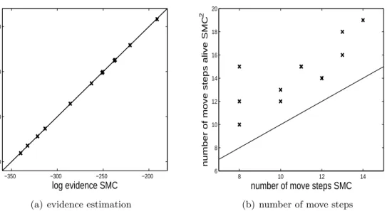
Figure 15 shows some additional results for all 12 datasets. From Figure 15(a) it is clear that using an unbiased likelihood estimator gives a log evidence estimate that is very similar to that of the ideal SMC algorithm that uses the true likelihood. Figure 15(b) demonstrates that the number of move steps required of alive SMC2 is always larger than that of the ideal SMC algorithm. This is due to the increase in variability of the importance weights when using a likelihood estimator; the inefficiency of alive SMC2 compared to ideal SMC. The number of unique particles at the end of alive SMC2 ranged between roughly 700-940 whereas the number of unique particles of the ideal SMC approach was typically 1000 (using the same value of R in both cases). This demonstrates a reduction in the MCMC acceptance rate of the move step when using an unbiased likelihood estimator as opposed to the true likelihood.
0 0.2 0.4 0.6 0.8 1
INAR(1) INAR(2) INMA(1) INARMA(1,1)
T
Model Probability
(a) model probs
0.1 0.2 0.3 0.4 0.5 0.6 0.7 0.8 0 1 2 3 4 5 6 7 8 9 α1 density alive SMC2 ideal SMC (b) α1 0.5 1 1.5 2 2.5 3 3.5 4 0 0.5 1 1.5 λ density alive SMC2 ideal SMC (c)λ 0.65 0.7 0.75 0.8 0.85 0.9 0.95 1 0 2 4 6 8 10 12 ρ density alive SMC2 ideal SMC (d) ρ
0 0.2 0.4 0.6 0.8 1
INAR(1) INAR(2) INMA(1) INARMA(1,1)
T
Model Probability
(a) model probs
0.1 0.2 0.3 0.4 0.5 0 1 2 3 4 5 6 7 8 α1 density alive SMC2 ideal SMC (b) α1 1 1.5 2 2.5 3 3.5 4 0 0.2 0.4 0.6 0.8 1 1.2 1.4 1.6 λ density alive SMC2 ideal SMC (c)λ 0.550 0.6 0.65 0.7 0.75 0.8 0.85 0.9 0.95 2 4 6 8 10 12 ρ density alive SMC2 ideal SMC (d) ρ
0 0.2 0.4 0.6 0.8 1
INAR(1) INAR(2) INMA(1) INARMA(1,1)
T
Model Probability
(a) model probs
0.2 0.25 0.3 0.35 0.4 0.45 0.5 0.55 0.6 0.65 0 1 2 3 4 5 6 7 8 9 α1 density alive SMC2 ideal SMC (b) α1 0.8 1 1.2 1.4 1.6 1.8 2 2.2 2.4 2.6 0 0.2 0.4 0.6 0.8 1 1.2 1.4 1.6 1.8 λ density alive SMC2 ideal SMC (c)λ 0.4 0.5 0.6 0.7 0.8 0 1 2 3 4 5 6 7 8 ρ density alive SMC2 ideal SMC (d) ρ
0 0.2 0.4 0.6 0.8 1
INAR(1) INAR(2) INMA(1) INARMA(1,1)
T
Model Probability
(a) model probs
0.1 0.2 0.3 0.4 0.5 0 1 2 3 4 5 6 7 8 α1 density (b) α1 0.1 0.2 0.3 0.4 0.5 0.6 0.7 0.8 0 1 2 3 4 5 6 7 8 α2 density (c) α2 0.5 1 1.5 2 2.5 3 3.5 0 0.2 0.4 0.6 0.8 1 1.2 1.4 λ density (d) λ 0.2 0.3 0.4 0.5 0.6 0.7 0.8 0.9 1 0 1 2 3 4 5 6 ρ density (e) ρ
0 0.2 0.4 0.6 0.8 1
INAR(1) INAR(2) INMA(1) INARMA(1,1)
T
Model Probability
(a) model probs
−0.050 0 0.05 0.1 0.15 0.2 0.25 0.3 0.35 0.4 1 2 3 4 5 6 7 8 α1 density (b) α1 0.2 0.25 0.3 0.35 0.4 0.45 0.5 0.55 0.6 0.65 0 1 2 3 4 5 6 7 α2 density (c) α2 0.5 1 1.5 2 2.5 3 3.5 0 0.2 0.4 0.6 0.8 1 1.2 1.4 λ density (d) λ 0.1 0.2 0.3 0.4 0.5 0.6 0.7 0.8 0.9 1 0 0.5 1 1.5 2 2.5 3 3.5 4 4.5 ρ density (e) ρ
0 0.2 0.4 0.6 0.8 1
INAR(1) INAR(2) INMA(1) INARMA(1,1)
T
Model Probability
(a) model probs
−0.10 0 0.1 0.2 0.3 0.4 0.5 0.6 1 2 3 4 5 6 7 α1 density (b) α1 0.1 0.2 0.3 0.4 0.5 0.6 0 1 2 3 4 5 6 7 α2 density (c) α2 0.5 1 1.5 2 2.5 3 3.5 0 0.2 0.4 0.6 0.8 1 1.2 1.4 1.6 1.8 2 λ density (d) λ 0.2 0.3 0.4 0.5 0.6 0.7 0.8 0.9 1 0 1 2 3 4 5 6 ρ density (e) ρ
0 0.2 0.4 0.6 0.8 1
INAR(1) INAR(2) INMA(1) INARMA(1,1)
T
Model Probability
(a) model probs
0.1 0.2 0.3 0.4 0.5 0.6 0 1 2 3 4 5 6 β1 density (b) β1 1 1.5 2 2.5 3 3.5 0 0.2 0.4 0.6 0.8 1 1.2 1.4 1.6 1.8 2 λ density (c)λ 0.450 0.5 0.55 0.6 0.65 0.7 0.75 0.8 0.85 0.9 1 2 3 4 5 6 7 8 9 10 rho density (d) ρ
0 0.2 0.4 0.6 0.8 1
INAR(1) INAR(2) INMA(1) INARMA(1,1)
T
Model Probability
(a) model probs
0.2 0.3 0.4 0.5 0.6 0.7 0 1 2 3 4 5 6 7 β1 density (b) β1 1 1.5 2 2.5 3 3.5 4 0 0.5 1 1.5 λ density (c)λ 0.65 0.7 0.75 0.8 0.85 0.9 0.95 0 2 4 6 8 10 12 rho density (d) ρ
0 0.2 0.4 0.6 0.8 1
INAR(1) INAR(2) INMA(1) INARMA(1,1)
T
Model Probability
(a) model probs
0.1 0.2 0.3 0.4 0.5 0.6 0.7 0.8 0 1 2 3 4 5 6 7 8 β1 density (b) β1 1 1.5 2 2.5 3 3.5 0 0.2 0.4 0.6 0.8 1 1.2 1.4 1.6 1.8 λ density (c)λ 0.450 0.5 0.55 0.6 0.65 0.7 0.75 0.8 0.85 0.9 2 4 6 8 10 12 rho density (d) ρ
0 0.2 0.4 0.6 0.8 1
INAR(1) INAR(2) INMA(1) INARMA(1,1)
T
Model Probability
(a) model probs
−0.10 0 0.1 0.2 0.3 0.4 0.5 0.6 0.7 1 2 3 4 5 6 α1 density (b) α1 0 0.1 0.2 0.3 0.4 0.5 0.6 0.7 0.8 0.9 0 0.5 1 1.5 2 2.5 3 3.5 4 4.5 β1 density (c)β1 1 1.5 2 2.5 3 3.5 0 0.2 0.4 0.6 0.8 1 1.2 1.4 1.6 1.8 λ density (d) λ 0.350 0.4 0.45 0.5 0.55 0.6 0.65 0.7 0.75 0.8 1 2 3 4 5 6 7 ρ density (e) ρ
0 0.2 0.4 0.6 0.8 1
INAR(1) INAR(2) INMA(1) INARMA(1,1)
T
Model Probability
(a) model probs
0.1 0.2 0.3 0.4 0.5 0.6 0.7 0.8 0 1 2 3 4 5 6 7 α1 density (b) α1 −0.20 0 0.2 0.4 0.6 0.8 1 1.2 0.5 1 1.5 2 2.5 3 3.5 β1 density (c)β1 0.5 1 1.5 2 2.5 3 0 0.5 1 1.5 λ density (d) λ 0.5 0.55 0.6 0.65 0.7 0.75 0.8 0.85 0.9 0 1 2 3 4 5 6 7 8 ρ density (e) ρ
0 0.2 0.4 0.6 0.8 1
INAR(1) INAR(2) INMA(1) INARMA(1,1)
T
Model Probability
(a) model probs
0 0.1 0.2 0.3 0.4 0.5 0.6 0.7 0 1 2 3 4 5 6 α1 density (b) α1 0 0.2 0.4 0.6 0.8 1 0 0.5 1 1.5 2 2.5 3 3.5 β1 density (c)β1 1 1.5 2 2.5 3 3.5 0 0.2 0.4 0.6 0.8 1 1.2 1.4 1.6 1.8 λ density (d) λ 0.4 0.5 0.6 0.7 0.8 0.9 0 1 2 3 4 5 6 7 8 9 ρ density (e) ρ
−350 −300 −250 −200 −350 −300 −250 −200 log evidence SMC
log evidence alive SMC
2
(a) evidence estimation
8 10 12 14 6 8 10 12 14 16 18 20
number of move steps SMC
number of move steps alive SMC
2
(b) number of move steps
Figure 15: Comparison of results and output from the SMC algorithm for the ZIP INAR(1) model when the exact likelihood is used and when an unbiased likelihood estimator is used (alive SMC2). Twelve simulated datasets are used to present the comparisons. (a) shows the log evidence estimation comparison and (b) shows the number of move steps required in the SMC algorithms for when exact and approximate likelihoods are used.
Appendix C
Here we show the parameter posterior distributions for the model with the highest posterior probability for each of the animal health time series datasets analysed in the main paper: (a) abort (Figure 16), (b) anorexia (Figure 17), (c) illthrift (Figure 18), (d) skin lesions (Figure 19) and (e) sudden death (Figure 20).
Appendix D
Given the current values of the states,S(t) =i,I(t) =j,L(t) =land C(t) =k, and a small time interval ∆t, the probabilities of various combinations of the states at timet+ ∆tfor the
0 0.1 0.2 0.3 0.4 0.5 0.6 0.7 0.8 0 0.5 1 1.5 2 2.5 3 3.5 4 4.5 α 1 density (a)α1 0.5 0.55 0.6 0.65 0.7 0.75 0.8 0.85 0.9 0 2 4 6 8 10 12 14 α 2 density (b) α2 0 0.5 1 1.5 2 2.5 3 0 0.2 0.4 0.6 0.8 1 1.2 1.4 λ density (c)λ 0.2 0.3 0.4 0.5 0.6 0.7 0.8 0.9 1 0 1 2 3 4 5 6 ρ density (d) ρ
Figure 16: Parameter posterior distributions of the ZIP INAR(2) model (highest posterior probability) applied to the abortion dataset.
0 0.1 0.2 0.3 0.4 0.5 0.6 0.7 0.8 0.9 0 0.5 1 1.5 2 2.5 3 3.5 4 α1 density (a)α1 0.550 0.6 0.65 0.7 0.75 0.8 0.85 0.9 0.95 2 4 6 8 10 12 α2 density (b) α2 0 1 2 3 4 5 6 7 8 0 0.1 0.2 0.3 0.4 0.5 0.6 0.7 λ density (c)λ 0.450 0.5 0.55 0.6 0.65 0.7 0.75 0.8 0.85 0.9 1 2 3 4 5 6 7 8 ρ density (d) ρ
Figure 17: Parameter posterior distributions of the ZIP INAR(2) model (highest posterior probability) applied to the anorexia dataset.
0.1 0.2 0.3 0.4 0.5 0.6 0 1 2 3 4 5 6 7 8 α1 density (a)α1 0.770 0.78 0.79 0.8 0.81 0.82 0.83 0.84 0.85 0.86 5 10 15 20 25 30 35 40 45 α2 density (b) α2 0 0.2 0.4 0.6 0.8 1 1.2 1.4 0 0.5 1 1.5 2 2.5 3 3.5 λ density (c)λ 0.2 0.3 0.4 0.5 0.6 0.7 0.8 0.9 0 1 2 3 4 5 6 ρ density (d) ρ
Figure 18: Parameter posterior distributions of the ZIP INAR(2) model (highest posterior probability) applied to the illthrift dataset.
−0.10 0 0.1 0.2 0.3 0.4 0.5 0.6 1 2 3 4 5 6 α1 density (a)α1 0.5 0.55 0.6 0.65 0.7 0.75 0.8 0.85 0.9 0 2 4 6 8 10 12 14 α2 density (b) α2 −0.20 0 0.2 0.4 0.6 0.8 1 1.2 1.4 1.6 0.2 0.4 0.6 0.8 1 1.2 1.4 1.6 1.8 2 λ density (c)λ 0 0.1 0.2 0.3 0.4 0.5 0.6 0.7 0.8 0 0.5 1 1.5 2 2.5 3 3.5 4 4.5 5 ρ density (d) ρ
Figure 19: Parameter posterior distributions of the ZIP INAR(2) model (highest posterior probability) applied to the skin lesion dataset.
−0.10 0 0.1 0.2 0.3 0.4 0.5 0.6 0.7 0.5 1 1.5 2 2.5 3 3.5 4 4.5 α1 density (a)α1 −0.20 0 0.2 0.4 0.6 0.8 1 1.2 0.5 1 1.5 2 2.5 β1 density (b) β1 0.5 1 1.5 2 2.5 3 3.5 4 4.5 0 0.2 0.4 0.6 0.8 1 1.2 1.4 λ density (c)λ 0.1 0.2 0.3 0.4 0.5 0.6 0.7 0.8 0 1 2 3 4 5 6 ρ density (d) ρ
Figure 20: Parameter posterior distributions of the ZIP INARMA(1,1) model (highest poste-rior probability) applied to the sudden death dataset.
P(S=i+ 1, L=l, I=j, C =k) =a∆t+o(∆t), P(S=i−1, L=l, I=j, C =k) =mi∆t+o(∆t), P(S=i−1, L=l+ 1, I =j, C =k) =βij∆t+o(∆t), P(S=i, L=l−1, I =j, C =k) =ml∆t+o(∆t), P(S=i, L=l−1, I =j+ 1, C =k) = µ αl∆t+o(∆t), P(S=i, L=l, I=j−1, C =k) =mj∆t+o(∆t), P(S=i, L=l, I =j−1, C =k+ 1) = µ 1−αj∆t+o(∆t). (4)
Appendix E
0 0.01 0.02 0.03 0.04 0.05 0.06 0.07 0.08 0.09 0 10 20 30 40 50 60 70 β density εt = 0 εt = 1 (a)β, direct −0.10 0 0.1 0.2 0.3 0.4 0.5 5 10 15 β density εt = 0 εt = 1 (b) β, latent 0 0.1 0.2 0.3 0.4 0.5 0.6 0.7 0.8 0 1 2 3 4 5 6 µ density εt = 0 εt = 1 (c) µ, direct 0 0.1 0.2 0.3 0.4 0.5 0.6 0.7 0.8 0.9 0 1 2 3 4 5 6 7 µ density εt = 0 εt = 1 (d) µ, latent −0.20 0 0.2 0.4 0.6 0.8 1 1.2 0.5 1 1.5 2 2.5 3 α density εt = 0 εt = 1 (e)α, latent