Partially Linear Functional Additive Models for Multivariate Functional Data

Statistics Publications Statistics

2018

Partially Linear Functional Additive Models for

Multivariate Functional Data

Raymond K.W. Wong

Texas A&M University

Yehua Li

Iowa State University, [email protected]

Zhengyuan Zhu

Iowa State University, [email protected]

Follow this and additional works at:https://lib.dr.iastate.edu/stat_las_pubs

Part of theMultivariate Analysis Commons, and theStatistical Models Commons

The complete bibliographic information for this item can be found athttps://lib.dr.iastate.edu/ stat_las_pubs/126. For information on how to cite this item, please visithttp://lib.dr.iastate.edu/ howtocite.html.

This Article is brought to you for free and open access by the Statistics at Iowa State University Digital Repository. It has been accepted for inclusion in Statistics Publications by an authorized administrator of Iowa State University Digital Repository. For more information, please contact

Partially Linear Functional Additive Models for Multivariate Functional

Data

Abstract

We investigate a class of partially linear functional additive models (PLFAM) that predicts a scalar response by both parametric effects of a multivariate predictor and nonparametric effects of a multivariate functional predictor. We jointly model multiple functional predictors that are cross-correlated using multivariate functional principal component analysis (mFPCA), and model the nonparametric effects of the principal component scores as additive components in the PLFAM. To address the high dimensional nature of

functional data, we let the number of mFPCA components diverge to infinity with the sample size, and adopt the COmponent Selection and Smoothing Operator (COSSO) penalty to select relevant components and regularize the fitting. A fundamental difference between our framework and the existing high dimensional additive models is that the mFPCA scores are estimated with error, and the magnitude of measurement error increases with the order of mFPCA. We establish the asymptotic convergence rate for our estimator, while allowing the number of components diverge. When the number of additive components is fixed, we also establish the asymptotic distribution for the partially linear coefficients. The practical performance of the proposed methods is illustrated via simulation studies and a crop yield prediction application.

Keywords

Additive model, Functional data, Measurement error, Reproducing kernel Hilbert space, Principal component analysis, Spline

Disciplines

Multivariate Analysis | Statistical Models | Statistics and Probability

Comments

This is an Accepted Manuscript of an article published by Taylor & Francis as Wong, Raymond KW, Yehua Li, and Zhengyuan Zhu. "Partially Linear Functional Additive Models for Multivariate Functional Data."Journal of the American Statistical Association(2018). Available online10.1080/01621459.2017.1411268. Posted with permission.

Full Terms & Conditions of access and use can be found at

http://amstat.tandfonline.com/action/journalInformation?journalCode=uasa20

Journal of the American Statistical Association

ISSN: 0162-1459 (Print) 1537-274X (Online) Journal homepage: http://amstat.tandfonline.com/loi/uasa20

Partially Linear Functional Additive Models for

Multivariate Functional Data

Raymond K. W. Wong, Yehua Li & Zhengyuan Zhu

To cite this article: Raymond K. W. Wong, Yehua Li & Zhengyuan Zhu (2018): Partially Linear Functional Additive Models for Multivariate Functional Data, Journal of the American Statistical Association, DOI: 10.1080/01621459.2017.1411268

To link to this article: https://doi.org/10.1080/01621459.2017.1411268

View supplementary material

Accepted author version posted online: 15 Jan 2018.

Submit your article to this journal

Article views: 148

Partially Linear Functional Additive Models

for Multivariate Functional Data

Raymond K. W. Wong1_{, Yehua Li}2 _{and Zhengyuan Zhu}2

1_{Department of Statistics, Texas A&M University, College Station, TX 77843}

2_{Department of Statistics & Statistical Laboratory, Iowa State University, Ames, IA 50011}

Abstract

We investigate a class of partially linear functional additive models (PLFAM) that pre-dicts a scalar response by both parametric effects of a multivariate predictor and nonpara-metric effects of a multivariate functional predictor. We jointly model multiple functional predictors that are cross-correlated using multivariate functional principal component anal-ysis (mFPCA), and model the nonparametric effects of the principal component scores as additive components in the PLFAM. To address the high dimensional nature of functional data, we let the number of mFPCA components diverge to infinity with the sample size, and adopt the COmponent Selection and Smoothing Operator (COSSO) penalty to select rele-vant components and regularize the fitting. A fundamental difference between our framework and the existing high dimensional additive models is that the mFPCA scores are estimated with error, and the magnitude of measurement error increases with the order of mFPCA. We establish the asymptotic convergence rate for our estimator, while allowing the number of components diverge. When the number of additive components is fixed, we also establish the asymptotic distribution for the partially linear coefficients. The practical performance of the proposed methods is illustrated via simulation studies and a crop yield prediction application.

Key Words: Additive model; Functional data; Measurement error; Reproducing kernel Hilbert space; Principal component analysis; Spline.

Short title: Partially Linear Functional Additive Models.

ACCEPTED MANUSCRIPT

1

Introduction

As new technology being increasingly used in data collection and storage, many variables are continuously monitored over time and become multivariate functional data (Ramsay and Silverman, 2005; Zhou et al., 2008; Kowal et al., 2017). Extracting useful information from such data for further regression analysis has become a challenging statistical problem. There has been significant amount of recent work devoted to regression models with functional predictors and the most popular model is the functional linear model (James, 2002; Cardot et al., 2003; M¨uller and Stadtm¨uller, 2005; Cai and Hall, 2006; Crainiceanu et al., 2009; Li et al., 2010; Cai and Yuan, 2012), where the scalar response variable is assumed to depend on an L2 _{inner product of the functional predictor with an unknown coefficient function.}

Functional data are infinite dimensional vectors in a functional space (Hsing and Eubank, 2015). Due to the richness of information in such data, a simple linear model is often found inadequate and many researchers have investigated nonlinear functional regression models. The most widely used approach is to project functional data into a low-rank functional sub-space and use the projections as predictors in a nonlinear model (James and Silverman, 2005; Li and Hsing, 2010a; Yao et al., 2016). The most popular and best understood dimension reduction tool for functional data is the functional principal component analysis (FPCA) (Yao et al., 2005; Hall et al., 2006; Li and Hsing, 2010b). A recent development in nonlinear functional regression model is the functional additive model (M¨uller and Yao, 2008; Zhu et al., 2014), where FPCA scores are used as predictors in an additive model.

Our research is motivated by a crop yield prediction application in agriculture. Agri-culture is a major industry in the U.S., the source of livelihood for millions of farmers and a vital contributor to global food security. Getting timely and reliable predictions on crop production is crucial for planners and policy makers to create appropriate strategies for the

1

ACCEPTED MANUSCRIPT

storage, distribution, and trade of agricultural products. The US National Agricultural Sta-tistical Service is the federal agency responsible for providing such statistics to the public, and their in-season crop yield forecast is primarily based on survey data. It is well known that weather has a significant impact on crop yield, and statistical models can be used to relate weather forcast to crop yield prediction (Cadson et al., 1996; Hansen, 2002; Prasad et al., 2006; Lobell and Burke, 2010). Since measurements of meteorological variables, such as maximum and minimum temperatures, are typically available on a daily basis and their effects on yield vary at different growing stage of the crop, it is natural to treat them as functional predictors. Besides the functional predictors, scalar predictors, such as crop man-agement methods, also have a great impact on yield and need to be included in the prediction model.

We propose a partially linear functional additive model (PLFAM) to predict a scalar response variable using both scalar and functional predictors. We use such a model to predict crop yield using the temperature trajectories. Such a model is of fundamental importance in plant science and agricultural economics: it advances our understanding of the relationship between weather conditions and crop yield, help to evaluate the impact of climate change on crop production and assist farmers and stake holders to better predict the future prices of agricultural commodity products and plan their actions accordingly. In many applications including our motivating data example, the functional predictors are strongly correlated to each other. To extract information more efficiently, we jointly model these predictors as a multivariate functional predictor, and perform dimension reduction using multivariate functional principal component analysis (mFPCA) (Ramsay and Silverman, 2005; Chiou et al., 2014). The proposed PLFAM includes the parametric effects of the scalar predictors and additive nonparametric effects of the mFPCA scores. To automatically select significant additive components, we impose COSSO penalties (Lin and Zhang, 2006) to the component

2

ACCEPTED MANUSCRIPT

functions and estimate the model in a reproducing kernel Hilbert space (RKHS) framework. Our approach is different from that of Zhu et al. (2014) in a few important perspectives. On the methodology side, we consider multiple functional predictors, extract informative sig-nals from the functional predictors using mFPCA, and we adopt a semiparametric partially linear structure in our model to take into account the effects of scalar predictors. On the the-ory side, we allow the number of additive components in the model to diverge to infinity with the sample size, to acknowledge the fact that functional data have infinite number of prin-cipal components. Our theory is fundamentally different from those in the high dimensional additive model literature, since our predictors in the additive model are estimated mFPCA scores that are contaminated with measurement errors (Carroll et al., 2006). As we show, the magnitude of measurement error gets higher for higher order principal components. In contrast, Zhu et al. (2014) only allow finite number of principal components in their model. To bound the effect of measurement errors, they also impose some very restrictive conditions which, in effect, limit their estimator in a finite dimensional subspace of the Sobolev space. Our results, on the other hand, does not rely on such artificial assumptions.

The rest of the paper is organized as follows. We describe the model and assumptions in Section 2 and the estimation procedure in Section 3. In Section 4 we investigate the asymptotic properties of the proposed estimator. We illustrate the proposed method with simulation studies in Section 5 and apply it to the motivating data example in Section 6. Some final remarks are collected in Section 7. Technical proofs and additional numerical results are relegated to the supplementary material.

3

ACCEPTED MANUSCRIPT

2

Model and Assumptions

Let Y be a scalar random variable associated with a predictor Z ∈ _Rp _{and a multivariate}

functional predictor X = (X1, . . . , Xd)|, where pand d are positive integers, andXj(t) is a

stochastic process defined on the time domain Tj for j = 1, . . . , d. For simplicity, we focus

on the case Tj ≡ T, but having different domains does not affect our methodological nor

theoretical developments. Let{zi,xi}ni=1 be i.i.d. copies of {Z,X}. Their relationship with the response {yi}ni=1 are modeled as

yi =m(zi,xi) +εi, i= 1, . . . , n, (1)

wheremis the regression function andεi are zero mean errors independent with{xi}ni=1 and {zi}ni=1. Further we assume var(εi) = σ2ε/πi, where σε2 is an unknown variance parameter

and πi’s are known positive weights. In our application, the responseyi is the averaged crop

yield per acre obtained from a survey, and πi is proportional to the size of the harvest land.

2.1

Multivariate functional principal component analysis

We assume that, with probability 1, the trajectory of Xj is contained in a Hilbert space

Xj, with inner product h·,·i_Xj and norm k · kXj. We will focus on the case that Xj’s are L

2

functional spaces and the inner products are hf, gi

Xj =

R

T f(t)g(t)dt for any f, g ∈Xj. Let X = Ldj=1Xj be the direct sum of the functional spaces, which is a bigger Hilbert space equipped with the induced inner product and norm, i.e. hx1,x2i_X =

Pd j=1hx1j, x2ji_Xj and kx1kX=hx1,x1i 1/2 X for any xi = (xi1, . . . , xid) |_∈ X, i= 1,2.

Define the mean function of the multivariate functional predictor as µ(t) = _E{X(t)}= {µ1(t), . . . , µd(t)}| where µj(t) =E{Xj(t)}. The cross-covariance function between Xj and

Xj0 is C_jj0(s, t) = _E[{X_j(s)−µ_j(s)}{X_j0(t)−µ_j0(t)}], and the covariance of X is a d×d

4

ACCEPTED MANUSCRIPT

matrix of cross-covariance functions

C(s, t) = _E[{X(s)−µ(s)}{X(t)−µ(t)}|_{] ={C}

jj0(s, t)}d_j,j0₌₁.

We assume thatC defines a bounded, self-adjoint, positive semi-definite integral operator (Hsing and Eubank, 2015). Standard operator theory warrants a spectral decomposition

C(s, t) =

∞ X

k=1

λkψk(s)ψ|_k(t),

where λ1 ≥ λ2 ≥ . . . > 0 are the eigenvalues and ψk = (ψk1, . . . , ψkd)| ∈ X are the

cor-responding eigenfunctions such that hψk,ψk0i X =

R

T ψk(t) |

ψk0(t)dt = I(k = k0). By a

standard Karhunen-Lo`eve expansion

X(t) = µ(t) +

∞ X

k=1

ξkψk(t),

whereξk =hX−µ,ψki_X are zero-mean random variables withE(ξkξk0) =λ_kI(k =k0). The

variables ξk are the mFPCA scores of X.

2.2

Partially linear functional additive model

Direct estimation of Model (1) suffers from the “curse-of-dimensionality” and is unpractical. Many popular alternative approaches are based on dimension reduction through FPCA and the effects of the functional predictors are modeled through their principal component scores, including the functional linear models (FLM) and the functional additive models (FAM). Our PLFAM model follows a similar strategy and can be considered as a special case of Model (1) with additional structural assumptions.

We denote the sequence of mFPCA scores of xi by ξi,∞ = (ξi1, ξi2, . . .)|. Even though

5

ACCEPTED MANUSCRIPT

in theory there are infinite number of principal components, the number of eigenfunctions estimated from the sample is at most n − 1, and as shown in our theory in Section 4.1 even fewer of eigenfunctions are estimated consistently. For these practical reasons, it is a common practice to only use the low-order FPCA scores as predictors in a regression. Denote the truncated mFPCA scores as ξi = (ξi1, . . . , ξis)|, with a positive integer s. To

avoid possible scale issues, we instead use the standardized versionζik = Φ(λ −1/2

k ξik), where

Φ(·) is a continuously differentiable map from _R to [0,1]. We let Φ(·) be the standard Gaussian cumulative distribution function (CDF) in all of our numerical studies. When the distribution ofξis close to Gaussian,ζis approximately uniform in [0,1], which is convenient for nonparametric modeling on the effect of ζ. Other continuous CDFs can also be used as Φ(·), such as the logistic function. Write ζi,∞ = (ζi1, ζi2, . . .) andζi = (ζi1, . . . , ζis).

Assuming that all useful information in the multivariate functional predictor is contained in the first s principal components, which are related to the response in an additive form, and the covariate effect is linear, then model (1) becomes the following Partially Linear Functional Additive Model (PLFAM)

yi =m0(ui,ζi) +εi =u|iθ0 +f0(ζi) +εi =u|iθ0+

s X

k=1

f0k(ζik) +εi, (2)

whereθ0 ∈Rp+1 andui = (1,zi|)|. Model (2) bears the functional additive model (FAM) of

M¨uller and Yao (2008) and Zhu et al. (2014) as a special case when the functional predictor

X(t) is univariate (d = 1) and there are no scalar covariates. The partially linear structure is widely used in many popular semiparametric models because it combines the flexibility of nonparametric modeling with easy interpretation of the covariate effects (Carroll et al., 1997; Liu et al., 2011; Wang et al., 2014). In practice, u can include interactions, quadratic terms and any other low order nonlinear terms as long as their effects are interpretable and

6

ACCEPTED MANUSCRIPT

parametric. We show in Section 4 the estimated partially linear coefficient θb(also referred

to as the parametric component of the model) is √n-consistent and has an asymptotically normal distribution, despite the existence of nonparametric components which converge in a slower rate. This is particularly useful if inference on the parametric effects is of primary interest in the study.

Following Lin and Zhang (2006) and Zhu et al. (2014), we assume that each f0k belongs

to a reproducing kernel Hilbert space (RKHS). We refer interested readers to Wahba (1990) for an introduction of RKHS for penalized regression. The most widely used RKHS is the Sobolev Hilbert space. In such context, an l-th order Sobolev Hilbert space _F(l)_{[0,1] is the} collection of functions on [0,1] whose first (l −1)-th derivatives are absolutely continuous and thel-th derivative belongs to L2_{[0,1], and the corresponding norm is chosen as}

kgk2 ₌ l−1 X v=0 Z 1 0 g(v)(t)dt 2 + Z 1 0 g(l)(t)2dt for any g ∈_F(l)_[0,1].

Let _Fk, k = 1, . . . , s, be a sequence of l-th order Sobolev spaces on [0,1] with reproducing

kernels Rk, and we assume f0k ∈ Fk. However, the fact that constant functions belongs to

each_Fk leads to an identifiability issue. To provide an identifiable parametrization, we note

that each _Fk has an orthogonal decomposition Fk ={1} ⊕F¯k where {1} is the space of all

constant functions. From now on, we assume m0 ∈ M = I⊕

Ps

k=1F¯k, where f0k ∈ F¯k for

k = 1, . . . , s, and _I ={u|_{θ : θ ∈}

Rp+1}. For the rest of the paper, we focus on the second

order Sobolev space with l = 2.

7

ACCEPTED MANUSCRIPT

3

Estimation and Computation

3.1

Estimation in mFPCA

To start with, we assume that the trajectories of xi(t)’s are fully observed. Then the mean

and covariance of X can be estimated by

b µ(t) = n−1 n X i=1 xi(t), Cb(s, t) =n−1 n X i=1 {xi(s)−µb(s)}{xi(t)−µb(t)} |_{. (3)}

Since Cbhas rankn−1, it has a spectral decomposition Cb(s, t) = Pn−1

k=1bλ_kψb_k(s)ψb|_k(t), where b

λk and ψb_k(t) are the sample eigenvalues and eigenfunctions. The estimated mFPCA scores

are b ξik =hxi,ψb_ki X = d X j=1 Z T xij(t)ψb_kj(t)dt, ζb_ik = Φ(bλ −1/2 k ξb_ik), k = 1, . . . , d. (4)

In practice, we only have discrete noisy observations on xi

wijk =xij(tijk) +eijk, i= 1, . . . , n, j = 1, . . . , d, k = 1, . . . , Nij,

whereeijk’s are independent measurement errors with mean 0 and varianceσe,j2 ,j = 1, . . . , d.

We will focus on the case where dense measurements are made on each curve such that each functional predictor can be effectively recovered by passing a linear smoother through the discrete observations. Let the recovered functions be x_eij(t) = S(t;tij)wij, where wij =

(wij1, . . . , wij,Nij)

| _{and S(t;t}

ij) is a linear smoother depending on the design points tij =

(tij1, . . . , tijNij)

|_{, e.g. local polynomial or regression splines. The eigenvalues, eigenfunctions} and mFPCA scores are estimated by replacing xij(t) withxeij(t) in (3) and (4).

For univariate functional data, this pre-smoothing approach is theoretically justified by Hall et al. (2006), who show that, whenSis a local linear smoother andNmin = mini,jNij >

8

ACCEPTED MANUSCRIPT

Cn1/4_{, the error incurred by approximating x}

ij(t) with exij(t) is negligible in bλk and ψbk; Li

et al. (2010) further show that this approximation error is negligible to ξb_ik if N_min > Cn5/4.

As commented in Li et al. (2010), there are two sources of error in ξb_ik: the error caused by

approximating xij with exij and the error in ψbk. If the first type of error prevails, regression

analysis using ξb_ik will be inconsistent even for linear models. The second type of error, on

the other hand, is diminishing to zero as n → ∞. There are mFPCA methodologies for sparse multivariate functional data (see e.g. Chiou et al. (2014)), but how to consistently estimate FAM or PLFAM when the estimated scores are contaminated with non-diminishing errors is not clear and calls for further research.

In all of our numeric studies, we smooth and register each xij on B-splines, pool spline

coefficients for each component inxiinto a longer vector, then the operatorCbis represented as

a high dimensional matrix, and the mFPCA problem reduces to a multivariate PCA problem. For detailed algorithm, we refer the readers to Section 8.5 in Ramsay and Silverman (2005).

3.2

Estimation of PLFAM with COSSO penalty

Letζb_i = (ζb_i1, . . . ,ζb_is)| be a vector of standardized mFPCA scores forx_i estimated using the

procedure in Section 3.1. Since there are potentially infinite number of principal components for X, we choose the truncation point s to be a large positive number and use a penalized regression method to select the relevant components.

The proposed estimator m_b is the minimizer of the following penalized loss `w(m) with

respect to m∈_M. The loss function is defined as

`w(m) = 1 n n X i=1 πi{yi−m(ui,ζb_i)}2+τ_n2J(m), (5)

where πi are the survey weights defined in (1). Here τn2 is a tuning parameter and J(m) =

9

ACCEPTED MANUSCRIPT

Ps

i=1kPkmkwithPkbeing the projection operator to ¯Fk. The penaltyJ(m) is first proposed in the COSSO framework (Lin and Zhang, 2006) for simultaneous estimation and selection of the nonparametric functions f0k’s.

Following Lin and Zhang (2006), we minimize (5) by iteratively minimizing its equivalent form 1 n n X i=1 πi{yi−m(ui,ζb_i)}2+κ₀ s X k=1 φ−_k1kPkmk2+κ s X k=1 φk (6)

overφ= (φ1, . . . , φs)|∈[0,∞)s and m∈M, whereκ0 >0 is a pre-determined constant and

κ is a tuning parameter.

The relationship between (5) and (6) is stated in the following lemma, which is an exten-sion of Lemma 2 in Lin and Zhang (2006) to partially linear additive model under a weighted least square loss. Its proof is omitted for brevity.

Lemma 1 (Lemma 2 of Lin and Zhang (2006)) Set κ=τ4

n/(4κ0). (i) If mb minimizes

(5), set φb_k=κ

1/2

0 κ

−1/2_kP

kmbk; then the pair (φb,mb) minimizes (6). (ii) If (φb,mb) minimizes

(6), then m_b minimizes (5).

By representer theorem, the minimizerm_b(u,ζ) takes the formu|_θ+Ps k=1φk

Pn

i=1aiRk(ζb_ik, ζ_k),

for u = (1, z1, . . . , zp)| ∈ Rp+1, (ζ1, . . . , ζs)| ∈ Rs, where a = (a1, . . . , an)| ∈ Rn is a vector

of unknown parameters. Then, minimization of (6) is equivalent to minimizing 1 nkΠ 1/2_{(y−U θ−} s X k=1 φkRka)k2E +κ0 s X k=1 φka|Rka+κ s X k=1 φk, (7)

where k · kE represents the Euclidean norm, Π = diag{π1, . . . , πn}, y = (y1, . . . , yn)|, U =

[uij]i=1,...,n,j=1,...,p+1 is a n×(p+ 1) design matrix and Rk = [Rk(ζbik,ζbjk)]i,j=1,...,n is a n×n

matrix for k = 1, . . . , s. For a fixed φ, minimizing (7) with respect to (θ,a) is similar to solving a weighted ridge regression. For fixed θ and a, let D be the n×s matrix with the

10

ACCEPTED MANUSCRIPT

k-th column being Rka, then minimization of (7) with respect to φ∈[0,∞)s becomes min1 n φ|D|ΠDφ−2 D|Π(y−U θ)− 1 2nκ0D |_a | φ subject to s X k=1 φk < G and φ∈[0,∞)s,

for some G > 0, which is a typical quadratic programming. The practical minimization of (5) is done by iterating over these two minimizations by fixing (θ,a) and φ in turn. The algorithm starts with solving (θ,a) while fixing φ= 1. Empirically, the objective function decreases quickly in the first iteration, which was also observed in Lin and Zhang (2006) and Storlie et al. (2011). To reduce the computational cost, we limit the number of iterations, and follow a one-step update procedure similar to Lin and Zhang (2006).

As discussed in Lin and Zhang (2006) and Storlie et al. (2011), κ0 can be fixed at any positive value. We select κ0 that minimizes the GCV of the partial spline problem when φ=1. Letφb(τn)= (φb

(τn)

1 , . . . ,φb

(τn)

n )|,a_b(τn)andθb(τn)be the minimizer of (7) for a fixedτ_n. To

select the smoothing parameterτn(or equivalentlyG), we minimize the Bayesian information

criterion nlog(RSSw(τn)/n) + df(τn) log(n), where the effective degress of freedom df(τn)

is the trace of the smoothing matrix in the partial spline problem (7) when φ is set to

b

φ(τn)_{, and the weighted residual sum of squares is RSS}

w(τn) = Pnn i=1πikΠ 1/2_{(y −U} b θ(τn)₋ Ps k=1φb (τn) k Rkab (τn)_)k2 E.

4

Theoretical Results

4.1

Basic results for mFPCA

By the theory of Dauxois et al. (1982), kC − Ckb op = Op(n−1/2) where the operator norm is

defined as kAkop = supx∈X

kAxk_X

kxk_X for any bounded linear operator A on X. To derive the

11

ACCEPTED MANUSCRIPT

asymptotic expansion for ξb_iks, we use the asymptotic expansion of bλ_k and ψb_k provided by

Hsing and Eubank (2015), which is a generalization of those by Hall and Hosseini-Nasab (2006) for univariate functional data to more general Hilbert space random variables. We adopt the following assumptions:

Assumption 1 (Cai and Hall (2006))

C_λ−1k−α ≤λk ≤Cλk−α, λk−λk+1 ≥C_λ−1k−1−α, k = 1,2, . . . . (8)

To ensure that P∞_k=1λk<∞, we assume that α >1.

Assumption 2 _E(kXk4

X) < ∞ and there exists a constant Cξ > 0 such that E(ξ

2

kξk20) ≤

Cξλkλk0 and _E(ξ2

k−λk)2 < Cξλ2k for all k and k 0 _6=k.

The polynomial decay rate described in Assumption 1 is a slow decay rate assumption on the eigenvalues and allows X(t) to be flexibly modeled as a multivariateL2 _{process without} strong constraints on the roughness of its sample path. Assumption 2 is a weak moment condition on the functional predictors and is satisfied if X(t) is a multivariate Gaussian process. Both assumptions are widely used in the functional linear model literature (Cai and Hall, 2006; Cai and Yuan, 2012; Hsing and Eubank, 2015). Defineδk = 1₂mink0_{=6 k}|λ_k0 −λ_k|,

which is no less than 1₂C_λ−1k−1−α _{under condition (8) and denote ∆ = n}1/2₍

b

C − C). By

Dauxois et al. (1982), ∆ converges weakly to a Gaussian variable in the space of linear operators and hence k∆kop =Op(1).

Proposition 1 (Transformed FPC scores) Suppose the transformation function Φ(·)

has bounded derivative. Under Assumptions 1 and 2, there is a constant C > 0 such that

E(ζb_ik−ζ_ik)2 ≤Ck2/n uniformly for k ≤J_n, where J_n=b(2C_λk∆k_op)−1/(1+α)n1/(2+2α)c.

12

ACCEPTED MANUSCRIPT

The proof of Proposition 1 is given in Appendix A in the supplementary material. It implies that the estimation error of the principal component score increases as the order of the principal component gets higher. Interestingly, the estimation error is of order Op(n−1/2k),

which does not depend on the decay rate α of the eigenvalues.

4.2

Asymptotic theory for PLFAM

For simplicity, we assume that πi = 1 for i = 1, . . . , n. We begin by introducing several

notations. We write Pn as the empirical distribution of (Z,ζ). That is, Pn = Pn

i=1δzi,ζi/n,

where δz,ζ is the delta function at (z,ζ). Moreover, we denote the distribution of (Z,ζ) by

P. We define the corresponding (squared) empirical norm and inner product as

km1k2n= Z

m2₁dPn and (m1, m2)n = Z

m1m2dPn, for any m1, m2 ∈M.

These notations are extended to measurement errors {εi}. For instance, (ε, m1)n = Pn

i=1εim1(ui,ζi)/n. Moreover, we write the Euclidean norm for vector as k · kE. To derive the asymptotic properties, we assume that the parametric component is identifiable. More specifically, Σ=R uu|_{dP is non-singular.}

Theorem 1 Suppose, for some β > 0, _E(ζb_ik −ζ_ik)2 ≤ Cn−1k2β uniformly for all k ≤ s.

Assume 0< J(m0)<∞, Σ is non-singular and τn−1 =Op(min{n2/5s−6/5, n1/2s−( 1

2+β)}), we

have km_b−m0kn=Op(τn)andJ(mb) =Op(1). IfJ(m0) = 0 andτnn

−1/4_s3_{, k} b m−m0kn= Op(n−1/2) and J(mb) =Op(n −1/2_s−6_). Remarks:

1. Under the framework laid out in Assumptions 1 and 2, with s=Op(n1/{2(1+α)}), we have E(ζb_ik −ζ_ik)2 ≤ Cn−1k2 uniformly for all k ≤ s followed from Proposition 1. The results in

Theorem 1 can be further simplified by identifying β = 1. In this case, if 0< J(m0)< ∞

13

ACCEPTED MANUSCRIPT

and τ−1

n =Op(n2/5s−6/5), we have kmb −m0kn =Op(n

−2/5_s6/5_{). If s is fixed, k}

b

m−m0kn =

Op(n−2/5) is the optimal nonparametric convergence rate assuming each f0k belongs to a

second order Sobolev space.

2. Our result can be considered as an extension of Theorem 1 in Zhu et al. (2014), where we allows→ ∞in a rate no faster thanOp(n1/{2(1+α)}). The reason for setting such a restriction

on the rate ofs is that, in order to estimate the principal components consistently, we need the distance between two adjacent eigenvalues to be no smaller than kC − Ckb op. This is a

fundamental difference with classic high dimensional additive models (Meier et al., 2009; Ravikumar et al., 2009; Liu et al., 2011; Wang et al., 2014).

3. The key issue in achieving consistent estimation of PLFAM is to bound the estimation error inζb_ik. To achieve this goal, Zhu et al. (2014) assumed (see their Assumption 1)

∂f(ζi) ∂ζik =|f_k0(ζik)| ≤Bikfk2 with probability 1

for some independent variables {Bi}ni=1 with E(Bi2) < ∞, where k · k2 is the L2(P)-norm. This is a strong assumption that eliminates the possibilityfk belonging to the space spanned

by high order Fourier or Demmler-Reinsch basis functions. As an effect, their estimation is restricted in a low dimensional functional space. We, on the other hand, show in Lemma 2 that sup_ζ∈[0,1]|f_k0(ζ)| is bounded by the RKHS norm of fk for all k ≤ s, and such a result

help to control the error caused by the error-contaminated predictor ζb_i.

When s is fixed, better asymptotic results can be derived for the regression coefficients

14

ACCEPTED MANUSCRIPT

γ = (γ1, . . . , γp)|= (θ2, . . . , θp+1)|. Define w(ζ) = (w1(ζ), . . . , wp(ζ))|= argmin _w j∈ {1} ⊕ Ps k=1F¯k j= 1, . . . , p EkZ−w(ζ)k2, e w(z,ζ) = (w_e1(z,ζ), . . . ,w_ep(z,ζ))|=z−w(ζ), M = (Mij)pi,j=1, where Mij = Z e wiwejdP. (9)

It is easy to see that w(ζ) defines a additive regression of Z onζ, and it can be considered as the projection of _E(Z|ζ) on the additive regression space, and therefore

E{we

|_{(z,ζ)g(ζ)}= 0 (10)}

for any g(ζ) = (g1, . . . , gp)|(ζ) such that gj(ζ)∈ {1} ⊕Ps_k=1F¯k for j = 1, . . . , p.

Theorem 2 Assume the conditions of Theorem 1 hold withs <∞ being fixed,ζ has a

non-degenerate joint density on [0,1]s _{which is bounded above and below, τ}

n = Op(n−1/4), and

thatM defined in (9) is non-singular. Then n1/2₍

b

γ−γ0)→Normal(000,M−1(V1+V2)M−1)

in distribution, where V1 and V2 are defined in (S.14) of the supplementary material.

Remark: As shown in our proof, V1 = cov{n1/2(ε,we)n}, and M −1_V

1M−1 is the typical asymptotic covariance matrix of γ_b in classic literature of partially linear additive model (Wang et al., 2014), where ζ is directly observed. The covariance V2 is the extra variation, caused by the estimation error in the FPCA score ζb. The two sources of variation are

asymptotically independent to each other because the model errorεis independent with the error inζb. A similar effect of FPCA estimation error was discovered by Li et al. (2010), who

investigated a simpler functional linear regression model and found that the FPCA error tends to inflate the asymptotic variance of the parametric component even if the functional predictors are fully observed. Our result in Theorem 2 shows the same phenomenon also

15

ACCEPTED MANUSCRIPT

exists for nonlinear functional regression models such as the PLFAM.

5

Simulation study

We extend the simulation setting of Zhu et al. (2014) to a multivariate functional data setting with an additional vector predictor Z. The multivariate functional predictor is xi(t) = {xi1(t), xi2(t)}| with xi1(t) = t+ sin(t) + P10 k=1ξ (1) ik ψ (1) k (t), xi2(t) =t+ cos(t) + P10 k=1ξ (2) ik ψ (2) k (t), where ξ_ik(1) ∼N(0, ς2k−1), ξ (2) ik ∼ N(0, ς2k), ςk = 45.25k−2, corr(ξ (j) ik , ξ (j) ik0) = 0 for k0 6= k, and

ψ_k(j)(t) = (1/√5) sin(πkt/10) for t ∈ T = [0,10], j = 1,2. The equations above define the univariate Karhunen-Lo`eve expansions for the two functional predictors respectively, scores within the same functional predictor are independent, however we allow the scores from different functional predictors to be cross-correlated. We let corr(ξ_ik(1), ξ_ik(2)0) = % for k0 = k

and 0 otherwise, where %is a cross-correlation parameter between 0 and 1.

The mFPCA eigenfunctions are defined through an orthogonalization of the univariate eigenfunctions, as described in Proposition 5 in Happ and Greven (2017). More specifi-cally, suppose the covariance matrix pooling all univariate FPCA scores has the eigenvalue decomposition var{(ξ(1)_i )|_,(ξ(2) i )|}| = P QP|_{, where ξ}(j) i = (ξ (j) i1 , . . . , ξ (j) i10)|, j = 1,2, Q = diag{λ1, . . . , λ20} and P|P = I. The k-th mFPCA score ξik ∼ N(0, λk) is a linear

function of the univariate scores{(ξ_i(1))|_,(ξ(2)

i )|}pk, wherepk ={(p

(1)

k )|,(p

(2)

k )|}|is thek-th

column of P, and the corresponding mFPCA eigenfunction is ψk(t) = (ψk1, ψk2)|(t), where

ψkj(t) = {ψ(j)(t)}|p (j) k , ψ(j)(t) = (ψ (j) 1 , . . . , ψ (j) 10)|(t), j = 1,2.

From model (2), we simulate 1000 i.i.d. copies of{Y,Z,X(·)}, denoted as{yi,zi,xi(·)}1000i=1 , with the first 200 used as training data and the rest as testing data. Observations onxi are

16

ACCEPTED MANUSCRIPT

obtained on a regular grid of 100 points inT = [0,10] with independent measurement errors following N(0,0.22). For the regression function, we setf0(ζ) = f01(ζi1) +f02(ζi2) +f04(ζi4), where f01(ζ1) = 3ζ1 −3/2, f02(ζ2) = sin{2π(ζ2 −1/2)} and f04(ζ4) = 8(ζ4 −1/3)2 −8/9. There are only three non-zero additive component functions in our simulation: f0k(ζk) = 0

for k /∈ {1,2,4}. Moreover, we generate the vector predictor zi independently from the

bivariate uniform distribution over [0,1]2_{. We consider two settings for the partially linear} coefficientθ0: (I) (1.4,0,0)| and (II) (1.4,3,−4)|and two settings of the correlation param-eter%: (i) 0.3 (low correlation) and (ii) 0.9 (high correlation). Combining different setups for

% and θ0, we have four settings: {(i), (I)}, {(i), (II)}, {(ii), (I)} and {(ii), (II)}. The errors

εi’s in the regression model (2) are distributed independently as N(0, σ2) withσ2 being 1 for

setting (I) and 1.9470 for (II) to achieve the signal-to-noise ratio (SNR) of approximately 2.2. The SNR is defined as var(m0(ζ))/var(ε). For simplicity, all sampling weightsπi are set

to be 1. The simulation is repeated 200 times and we fit the following two models to each simulated data set: FAM of Zhu et al. (2014), which is also based on COSSO but ignores the effect of Z, and the proposed PLFAM. Throughout this simulation study, s is chosen to recover at least 99.9% of the total variation in {xi} and the COSSO tuning parameters are

selected by the Bayesian information criterion.

Tables 1 and 2 summarize the results related to component function selection in FAM

andPLFAMunder the four settings. Due to space constraint, only percentages of model sizes up to 8 and selection percentages of the first 8 component functions are shown. In Table 2, Column “% correct set” corresponds to the percentages of fittings achieving exact selection of fb₁ fb₂ and fb₄, while Column “% super set” gives the percentages of fittings that include

nonzero fb₁, fb₂ and fb₄. Despite a small tendency of over-selection, the COSSO component

selection mechanism tends to select parsimonious models and, for each correct component function, the selection percentage is high.

17

ACCEPTED MANUSCRIPT

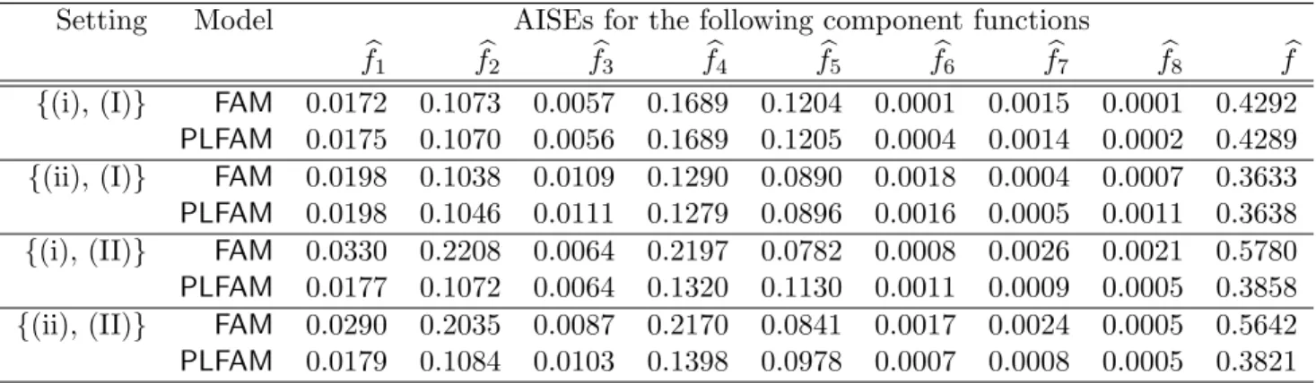
To assess the estimation quality of f0k’s, Table 3 shows the averaged integrated squared

errors (AISEs) of the first eight component functions and the overall function fb= Ps

k=1fb_k

(without constant term). The integrated squared errors are defined as

ISE(fb_k) = Z 1 0 {fb_k(t)−f_0k(t)}2dt and ISE(fb) = s X k=1 Z 1 0 {fb_k(t)−f_0k(t)}2dt.

Notice that, under setting (I) where Z has zero effect and FAM is the correct model, the

PLFAMestimators perform comparably to those of FAM. However, under setting (II), where Z has non-zero effects, FAM performs significantly worse than PLFAM. This demonstrates the possible risk of ignoring important vector predictors.

We also summarize the prediction errors, and the mean squared errors (MSE) for the estimated partially linear coefficients in Table 4. To show the advantage of mFPCA, we further compare two methods to obtain FPCA scores: the “joint” approach is the mFPCA approach that we advocate; and the “separate” approach is to perform univariate FPCA to each component of X, standardize these scores separately, and then pool all standardized scores together as covariates in the additive model. Both FPCA approaches can be used in conjunction with FAM and PLFAM. The prediction error is computed by n−1Pn

i=1(yi−ybi)

2

on the testing data set. To compute the prediction y_bi in the test data, we first compute

the transformed FPCA scores of xi in the test set using the estimates of mean function,

eigenvalues and eigenfunctions from the training data, and then plug these scores into the estimated regression m_b. The results in Table 4 suggest that jointly modeling multiple func-tional predictors leads to smaller MSE’s for θb, and lower prediction errors, as opposed to

modeling each functional predictor separately using univariate FPCA. In addition, PLFAM

has significant lower prediction errors than FAM under setting (II) when there is a non-zero effect from Z.

18

ACCEPTED MANUSCRIPT

In Section C of the supplementary material, we also report the simulation results when s

chosen to recover 90% of the total variation. Under this setting, one important component related to Y is close to the 90% cut-off line and often not included as a candidate for COSSO. As a results, a non-zero component function is often failed to be selected, and the resulted models yield higher prediction errors in the test data sets. Based on these results, we recommend to include a large number of components and let the built-in model selection mechanism of COSSO determine the size of the model.

6

Real Data Application

The practical utility of the proposed method is illustrated through an analysis of a crop yield data set from the National Agricultural Statistics Agency (https://quickstats.nass.usda.gov/), which consists of several yield-related variables at the county level (such as annual crop yield in bushels per acre, size of harvested land and the proportion irrigated land to the total har-vested land) from 105 counties in Kansas from 1999 to 2011. We have yield-related variables for the two major crops in Kansas, corn and soybean, which are analyzed separately. Vari-ables such as total harvest land and proportion of irrigated land are crop-specific. The weather data (annual averaged precipitation, daily maximum temperature and daily min-imum temperature) are gathered from 1123 weather stations in Kansas provided by the National Climatic Data Center (https://www.ncdc.noaa.gov/data-access) and aggregated at the county level.

To apply our model, let Y be the average crop yield per acre (corn or soybean) for a specific year and county; X1(t) and X2(t) are the daily maximum and daily minimum temperature trajectories for the same year and county with the time domain T = [0,365]; Z includes proportion of irrigated land in that county and for that particular type of crop,

19

ACCEPTED MANUSCRIPT

averaged annul precipitation, and the interaction between the two. In the past several decades, due to sustained improvements in genetics and production technology, there is a consistent increasing trend in the yields of both corn and soybean. To take this effect into consideration, we also include year indicators into Z.

Since the response is an average obtained from an agricultural survey, the errors are heteroscedastic with weights π equal to the sizes of harvested land. Some earlier work (Smith, 1938; Beran et al., 2013) suggests crop yield may exhibit long range dependency on a scale measured in feet. Our study on the other hand is based on county level aggregated data. The crop yields are usually averaged over tens of thousands of acres within a county and not from a continuous piece of land. At this scale, the spatial correlation is already quite weak and therefore it is reasonable to assume the variance of the average crop yield is proportional to the inverse of the total harvest land. Furthermore, land use rotates between the major crops across years: land used to grow corn this year is usually used to grow soybean the next year. Variables such as the proportion of irrigated land and size of harvest land are different in different years even for the same crop and same county. Even though our theory and methods are developed under the independence assumption, they can still be applied as long as the crop yields are conditionally independent across counties and years, given the local meteorology information, which seems reasonable because of the rotation in land use and because crops of different genotypes are planted in different years.

To illustrate the functional predictors, we show in Figure S.1 of the supplementary ma-terial 50 randomly selected trajectories for X1(t) and X2(t), with the mean functions µ1(t) and µ2(t) marked as solid curves in the two panels. As one can see, there are a lot of local fluctuations in the temperature trajectories, which is normal since heat and chill alternate throughout the year. In Figure 1, we show the heat plots for the (cross-) covariance func-tions. The kernel function for C12 shows great resemblance to C11 and C22, which implies

20

ACCEPTED MANUSCRIPT

that the two functional predictors are strongly correlated. This also suggests mFPCA would achieve more efficient dimension reduction than univariate FPCA done separately to the two processes, and the latter would include too much redundant information into the regression model.

6.1

Crop yield prediction experiment

Since our goal of this study is to find the best model for yield prediction, we divide the data into smaller training and validation data sets and compare the prediction of the following 10 competing models.

1. PLFAM(joint): the proposed PLFAM based on mFPCA scores;

2. PLFAM(separate): PLFAM based on univariate FPCA scores from X1 and X2 sepa-rately;

3. FAM(joint): FAM based on mFPC scores (without Z);

4. FAM(separate): FAM based on univariate FPC scores (without Z);

5. FLM-Cov(joint): functional linear model (FLM) based on mFPCA scores, with covari-ates;

6. FLM-Cov(separate): FLM based on separate univariate FPCA scores, with covariates;

7. FLM(joint): FLM based on joint mFPCA scores (without Z); 8. FLM(separate): FLM based on separate FPCA scores (without Z); 9. LM: linear model on Z only;

10. LM-GDD: linear model onZ and Growing Degree Days (GDD), to be explained below.

21

ACCEPTED MANUSCRIPT

The models we consider can be divided into three categories: (a) functional additive models (Models 1-4), (b) functional linear models (Models 5-8) and (c) non-functional model (Models 9 - 10). For all functional regression models, including those in categories (a) and (b), FPCA scores that account up to 99.9% of the total variation are admitted into the model. For the methods based on separate FPCA on X1 and X2, we include FPCA scores that explain 99.9% of total variation in each functional predictor and thus use twice as many FPCA scores in the regression analysis as the joint modeling methods. For all models in category (a), we rely on the model selection mechanism of COSSO to prevent overfitting and select the tuning parameters by 5-fold cross-validation; for the functional linear models in category (b), we avoid overfitting by introducing ridge penalties, the tuning parameters of which are chosen by generalized cross-validation. It is worth noting that Model 10 serves as the benchmark model for yield prediction with temperature information enters into the model as the GDD variable. GDD is a measure of heat accumulation commonly used to predict plant development (Gilmore and Rogers, 1958; Yang et al., 1995; McMaster and Wilhelm, 1997). Here we adopt the definition used in the EPIC (Erosion Productivity Impact Calculator) plant growth model (Williams et al., 1989), in which GDD is defined as the sum of [{X1(t) +X2(t)}/2−Tbase]+ over growing season, where Tbase is the crop-specific

base temperature in ◦C. For corn Tbase = 8, and for soybean Tbase = 10. To account for

heteroscedasticity, the sizes of harvested land are used as weights in fitting all models. For each five-year window (i.e., 1999-2003, 2000-2004, . . . , 2007-2011), we pull the data from those five years into a smaller data set. For each five-year data set, we randomly divide it into five subsets, hold out one subset at a time as a validation set, fit the ten models described above to the remaining four subsets, and then use the trained models to predict the responses in the validation data. The mean squared prediction errors are weighted by the sizes of harvested land, averaged over the five validation sets and over all five-year

22

ACCEPTED MANUSCRIPT

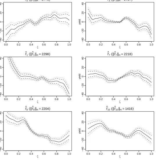
periods. The averaged overall prediction errors are reported in Table 5. From the table, models without the covariate effects, including FAM(separate), FAM(joint), FLM(separate)

and FLM(joint), perform significantly worse than the rest. These results agree with the general belief that irrigation and precipitation are informative in yield prediction, which also stress the importance of extending the FAM of M¨uller and Yao (2008) to our PLFAM. We can also see that including the functional predictors can reduce the prediction error, and functional regression model such asPLFAM(separate), PLFAM(joint),FLM-Cov(separate) and

FLM-Cov(joint) perform better than the non-functional models (LM and LM-GDD). Joint modeling the two functional predictors using mFPCA also leads to lower prediction error for both PLFAM and FLM-Cov. Overall, PLFAM(joint) performs the best in corn yield prediction and achieves comparable result to FLM-Cov(joint) for soybean.

Part of the reason that PLFAM performs slightly worse than FLM in soybean yield prediction is that the nonlinear effect is less significant for soybean and PLFAM requires a larger sample size. In another experiment where we include more years of data in the training set, PLFAM predicts soybean yield better than FLM.

In addition to the 10 models described above, we also consider another 12 models that use X1, X2 or (X1 +X2)/2 alone. These models yield higher prediction errors than the proposed PLFAM(joint) model, which utilizes both functional predictors. Even though the two functional covariates in the real data are strongly correlated as suggested by Figure 1, these results show that each covariate does provide additional information that complements the other and it is beneficial to jointly model them. Due to space limitation, these results are presented in Section D of the supplementary material.

23

ACCEPTED MANUSCRIPT

6.2

Regression analysis of the whole data

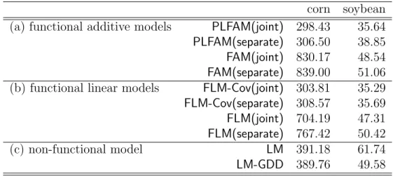
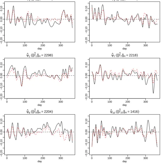
We now apply PLFAM(joint) to the whole data set pooling all available years. For corn yield prediction, we include 52 principal components in the regression model which account for ∼ 99% of variation in the temperature trajectories, and 10 principal components are selected by COSSO. In Figure 2, we show the top 6 most significant principal components; and in Figure 3, we show the corresponding additive component functions fb_k(ζ). These

components are ranked by the importance of their contribution to Y. More specifically, we sort the principal components by the RKHS norm of the component functionfbk. The dashed

curves in Figure 3 are the pointwise confidence bands fb_k(ζ)±2×se{fb_k(ζ)}, and the dotted

curves are the 3 times standard error bands. The standard errors are estimated using a bootstrap procedure detailed in the supplementary material.

Since each principal component in mFPCA is a vector of functionsψk(t) = {ψk1(t), ψk2(t)}|, we show ψk1(t) as the solid curve and ψk2(t) as the dashed curve in each panel of Figure 2. It is not surprising that ψk2(t) largely coincides with ψk1(t), given the observation from the covariance functions that the two processes are strongly correlated. However, the plots do reveal subtle differences between the two temperature trajectories. The component most related to corn yield ψ5 features a temperature pattern with near average daily minimum temperature and lower than average daily maximum temperature during the summer months from May to September. A higher loading on ψ5 means a milder summer, less heat stress and less chance of draught, and corn yield is an increasing function of ζ5 in Figure 3. In contrast, ψ1 and ψ8 represent hot summers, and crop yield is a decreasing function of their loadings ζ1 and ζ8. These are consistent with the findings in Westcott et al. (2013), which conclude that hot July - August weather lowered the corn yield. A prominent feature inψ3 is warm spring months from January to March, which may lead to less snow coverage on the ground, early insect activities and hence the negative association with corn yield as described

24

ACCEPTED MANUSCRIPT

byf3(ζ) in Figure 3. For soybean yield prediction, graphs of the selected eigenfunctions and the corresponding additive component functions are similar to those in Figures 2 and 3, and are hence omitted.

The estimated partially linear coefficients and their bootstrap standard errors for both corn and soybean yield models are summarized in Table 6. As we can see, both the proportion of irrigated land (Irrigate) and precipitation (Prec) have signifiant positive effects on crop yield. The significant negative interaction means the effect of Prec is mitigated when a big portion of the lands in the county are equipped with irrigation systems. For corn yield prediction, the first and third quartiles for Irrigateare 0.027 and 0.485 respectively. Changing Irrigate from its first quartile to the third, the partial slope on Prec reduces from 167.47 to 151.95.

The bootstrap procedure, provided in the supplementary material, is based on the as-sumption that the errors in model (2) are independent. To validate this asas-sumption, we also estimate the spatial variogram for each year and temporal autocorrelation for each county based on the residuals of the fitted model, see Figures S.2 and S.3 in the supplementary material. The variograms and ACF’s are contained in their confidence bands based on the assumption of no dependency, which means there is no significant evidence for spatial or temporal correlation.

7

Concluding Remarks

7.1

Our contributions

We have extended the FAM of M¨uller and Yao (2008) to a class of PLFAM which takes into account of the effects of a multivariate covariate Z. As demonstrated in our crop yield application, including the covariate effects significantly improves the prediction accuracy.

25

ACCEPTED MANUSCRIPT

The effect of functional predictors are modeled through an additive model on the principal component scores. Since the FPC scores are estimated with error, our theory and methods also shine a new light on the area of additive models with covariate measurement errors.

We have also made a number of important theoretical contributions. First, we develop a more general model framework which includes multivariate functional predictors and mul-tivariate covariates. Second, we allow the number of principal components admitted in the additive model to diverge to infinity, which is fundamentally different from Zhu et al. (2014). Third, we are able to quantify and bound the nuisance from the estimation errors in mF-PCA scores without the artificial assumption in Zhu et al. (2014). Finally, when the number of principal components does not diverge to infinity, we establish root-n consistency and asymptotic normal distribution for the partially linear regression coefficients.

7.2

Interpretability of the model

Functional regression models based on principal components are in general hard to interpret, because FPC’s are the maximum modes of variation in the functional predictors which are not necessarily the features most related to the response variable. This is part of the reason that many authors focused on prediction using functional linear model (Cai and Hall, 2006; Cai and Yuan, 2012). Our proposed PLFAM adopts the philosophy of semiparametric statis-tics: we model the effects of functional covariates nonparametrically to increase the model flexibility and prediction performance, and model the effects of the multivariate covariates parametrically for better interpretations and statistical inference. Our Theorem 2 provides a basis for statistical inference on the parametric componentγ. There is also another class of functional additive regression models proposed by M¨uller et al. (2013); McLean et al. (2014); Kim et al. (2017), which offer an alternative view on modeling nonlinear effects of functional covariates.

26

ACCEPTED MANUSCRIPT

7.3

mFPCA versus separate FPCA

For multivariate functional data, mFPCA usually provides more efficient dimension reduction than separate FPCA to each functional covariate. However, mFPCA estimates are subject to higher variability due to the need of estimating all cross-covariance functions and performing eigenvalue decomposition on a much larger covariance matrix. When the sample size is small, the extra variation in mFPCA can offset its benefit. There are also other situations where separate FPCA is more preferable, such as when different functional covariates are of different scales or even defined on different domains (Happ and Greven, 2017). Under these situations, our theory and methods can also be easily extended to the model based on separate FPCA scores. A separate FPCA version of model (2) is

yi =u|iθ0+ s X k=1 d X j=1 f0jk(ζijk) +εi, (11)

where ζijk is the kth standardized principal component score for xij. The model can be

fitted using the same COSSO algorithm described in Section 3.2 except that the mFPCA scores are replaced by the separate FPCA scores. As long as the separate FPC scores can be estimated with a similar accuracy as assumed in Theorem 1, i.e. _E(ζb_ijk−ζ_ijk)2 ≤Cn−1k2β

uniformly for all j = 1, . . . , d and k ≤s, the same asymptotic results in Theorems 1 and 2 hold for the model in (11).

Acknowledgement

Wong’s research was partially supported by the National Science Foundation under Grants DMS-1612985 and DMS-1711952 (subcontract). Li’s research was partially supported by the National Science Foundation grant DMS-1317118. Zhu’s research was funded in part by cooperative agreement 68-7482-17-009 between the USDA Natural Resources Conservation

27

ACCEPTED MANUSCRIPT

Service and Iowa State University.

References

Beran, J., Feng, Y., Ghosh, S., and Kulik, R. (2013). Long-Memory Processes. Springer, New York.

Brezis, H. (2010). Functional analysis, Sobolev spaces and partial differential equations. Springer, New York.

Cadson, R., Todey, D. P., and Taylor, S. E. (1996). Midwestern corn yield and weather in relation to extremes of the southern oscillation. Journal of Production Agriculture, 9(3):347–352.

Cai, T. T. and Hall, P. (2006). Prediction in functional linear regression. The Annals of Statistics, 34(5):2159–2179.

Cai, T. T. and Yuan, M. (2012). Minimax and adaptive prediction for functional linear regression. Journal of the American Statistical Association, 107:1201–1216.

Cardot, H., Ferraty, F., and Sarda, P. (2003). Spline estimators for the functional linear model. Statistica Sinica, 13:571–591.

Carroll, R. J., Fan, J., Gijbels, I., and Wand, M. P. (1997). Generalized partially linear single-index models. Journal of the American Statistical Association, 92(438):477–489. Carroll, R. J., Ruppert, D., Stefanski, L. A., and Crainiceanu, C. M. (2006). Measurement

Error in Nonlinear Models: A Modern Perspective. Chapman and Hall/CRC, Boca Raton,

FL.

Chiou, J.-M., Y.-T., C., and Yang, Y.-F. (2014). Multivariate functional principal component analysis: a normalization approach. Statistica Sinica, 24:1571–1596.

Crainiceanu, C. M., Staicu, A.-M., and Di, C.-Z. (2009). Generalized multilevel functional regression. Journal of the American Statistical Association, 104:155–1561.

Dauxois, J., Pousse, A., and Romain, Y. (1982). Asymptotic theory for the principal com-ponent analysis of a vector random function: some applications to statistical inference.

Journal of Multivariate Analysis, 12(1):136–154.

Gilmore, E. and Rogers, J. (1958). Heat units as a method of measuring maturity in corn.

Agronomy Journal, 50(10):611–615.

Hall, P. and Hosseini-Nasab, M. (2006). On properties of functional principal components analysis. Journal of the Royal Statistical Society: Series B, 68(1):109–126.

Hall, P., M¨uller, H. G., and Wang, J. L. (2006). Properties of principal component methods for functional and longitudinal data analysis. Annals of Statistics, 34:1493–1517.

28

ACCEPTED MANUSCRIPT

Hansen, J. W. (2002). Realizing the potential benefits of climate prediction to agriculture: issues, approaches, challenges. Agricultural Systems, 74(3):309–330.

Happ, C. and Greven, S. (2017). Multivariate functional principal component analysis for data observed on different (dimensional) domains. Journal of American Statistical Asso-ciation, page to appear.

Hollinger, S. E., Changnon, S. A., et al. (1994). Response of corn and soybean yields to precipitation augmentation, and implications for weather modification in illinois.

Bul-letin/Illinois State Water Survey; no. 73.

Hsing, T. and Eubank, R. (2015).Theoretical Foundations of Functional Data Analysis, with

an Introduction to Linear Operators. Wiley.

James, G. (2002). Generalized linear models with functional predictor variables. Journal of

the Royal Statistical Society, Series B, 64:411–432.

James, G. and Silverman, B. W. (2005). Functional adaptive model estimation. Journal of

the American Statistical Association, 100:565–576.

Kim, J., Staicu, A.-M., Maity, A., Carroll, R. J., and Ruppert, D. (2017). Additive function-on-function regression. Journal of Computational and Graphical Statistics, to appear. Kowal, D. R., Matteson, D. S., and Ruppert, D. (2017). A bayesian multivariate functional

dynamic linear model. Journal of the American Statistical Association, 112:733–744. Li, Y. and Hsing, T. (2010a). Deciding the dimension of effective dimension reduction space

for functional and high-dimensional data. Annals of Statistics, 38:3028–3062.

Li, Y. and Hsing, T. (2010b). Uniform convergence rates for nonparametric regression and principal component analysis in functional/longitudinal data. Annals of Statistics, 38:3321–3351.

Li, Y., Wang, N., and Carroll, R. J. (2010). Generalized functional linear models with semiparametric single-index interactions. Journal of the American Statistical Association, 105:621–633.

Lin, Y. and Zhang, H. H. (2006). Component selection and smoothing in multivariate nonparametric regression. The Annals of Statistics, 34(5):2272–2297.

Liu, X., Wang, L., and Liang, H. (2011). Estimation and variable selection for semiparametric additive partial linear models. Statistica Sinica, 21:1225–1248.

Lobell, D. B. and Burke, M. B. (2010). On the use of statistical models to predict crop yield responses to climate change. Agricultural and Forest Meteorology, 150(11):1443–1452. Mammen, E. and van de Geer, S. (1997). Penalized quasi-likelihood estimation in partial

linear models. The Annals of Statistics, 25(3):1014–1035.

McLean, M. W., Hooker, G., Staicu, A. M., Scheipl, F., and Ruppert, D. (2014). Functional generalized additive models. Journal of Computational and Graphical Statistics, 23:249 – 269.

29

ACCEPTED MANUSCRIPT

McMaster, G. S. and Wilhelm, W. (1997). Growing degree-days: one equation, two inter-pretations. Agricultural and Forest Meteorology, 87(4):291–300.

Meier, L., van de Geer, S., and B¨uhlmann, P. (2009). High-dimensional additive modeling.

The Annals of Statistics, 37(6B):3779–3821.

M¨uller, H. G. and Stadtm¨uller, U. (2005). Generalized functional linear models. Annals of Statistics, 33:774–805.

M¨uller, H.-G., Wu, Y., and Yao, F. (2013). Continuously additive models for nonlinear functional regression. Biometrika, 103:607–622.

M¨uller, H.-G. and Yao, F. (2008). Functional additive models. Journal of the American

Statistical Association, 103(484):1534–1544.

Nirenberg, L. (1959). On elliptic partial differential equations. Annali della Scuola Normale

Superiore di Pisa-Classe di Scienze, 13(2):115–162.

Prasad, A. K., Chai, L., Singh, R. P., and Kafatos, M. (2006). Crop yield estimation model for iowa using remote sensing and surface parameters. International Journal of Applied

Earth Observation and Geoinformation, 8(1):26–33.

Ramsay, J. O. and Silverman, B. W. (2005). Functional data analysis. Springer, New York, 2nd edition.

Ravikumar, P., Lafferty, J., Liu, H., and Wasserman, L. (2009). Sparse additive models.

Journal of the Royal Statististical Society, Series B, pages 1009–1030.

Smith, H. F. (1938). An empirical law describing heterogeneity in the yields of agricultural crops. Journal of Agricultural Science, 28:1–23.

Storlie, C. B., Bondell, H. D., Reich, B. J., and Zhang, H. H. (2011). Surface estimation, variable selection, and the nonparametric oracle property. Statistica Sinica, 21(2):679. van de Geer, S. (2000). Empirical Processes in M-estimation. Cambridge University Press,

New York.

Wahba, G. (1990). Spline Models for Observational Data. SIAM, Philadelphia.

Wang, L., Xue, L., Qu, A., and Liang, H. (2014). Estimation and model selection in general-ized additive partial linear models for correlated data with diverging number of covariates.

Annals of Statistics, 42:592–624.

Westcott, P. C., Jewison, M., et al. (2013). Weather effects on expected corn and soybean yields. Washington DC: USDA Economic Research Service FDS-13g-01.

Williams, J., Jones, C., Kiniry, J., and Spanel, D. (1989). The epic crop growth model.

Transactions of the ASAE, 32(2):497–0511.

Yang, S., Logan, J., and Coffey, D. L. (1995). Mathematical formulae for calculating the base temperature for growing degree days. Agricultural and Forest Meteorology, 74(1):61–74.

30

ACCEPTED MANUSCRIPT

Yao, F., Lei, E., and Wu, Y. (2016). Effective dimension reduction for sparse functional data. Biometrika, page to appear.

Yao, F., M¨uller, H. G., and Wang, J. L. (2005). Functional data analysis for sparse longitu-dinal data. Journal of the American Statistical Association, 100:577–590.

Zhou, L., Huang, J. Z., and Carroll, R. J. (2008). Joint modelling of paired sparse functional data using principal components. Biometrika, 95:601–619.

Zhu, H., Yao, F., and Zhang, H. H. (2014). Structured functional additive regression in reproducing kernel hilbert spaces. Journal of the Royal Statistical Society: Series B, 76(3):581–603.

31

ACCEPTED MANUSCRIPT

Table 1: Percentages of fitted model sizes.

Setting Model % for the following model sizes

1 2 3 4 5 6 7 8

{(i), (I)} FAM 0 0 28 49.5 20.5 1.5 0.5 0

PLFAM 0 0 24 57.5 17 1 0.5 0

{(ii), (I)} FAM 0 0 20.5 58 16.5 4 1 0

PLFAM 0 0 19 58.5 18 3.5 0 1

{(i), (II)} FAM 0 6.5 41 39.5 12 0.5 0.5 0

PLFAM 0 0 22.5 56 18 3 0.5 0

{(ii), (II)} FAM 0 3 44.5 38 12.5 2 0 0

PLFAM 0 0 22.5 61 12.5 3 1 0

Table 2: Percentages of selected components and, correct and super selection.

Setting Model % for the following component functions % correct % super

b

f1 fb₂ fb₃ fb₄ fb₅ fb₆ fb₇ fb₈ set set

{(i), (I)} FAM 100 100 14 93 51.5 2 6 1.5 27 93

PLFAM 100 100 14 93 51.5 3 5 1.5 23 93

{(ii), (I)} FAM 100 100 20.5 97 51 5.5 1.5 2 18.5 97

PLFAM 100 100 20 97.5 53 5.5 1.5 2.5 17.5 97.5

{(i), (II)} FAM 100 90 8.5 93.5 34.5 2.5 4.5 4.5 35 83.5

PLFAM 100 100 16 97.5 54.5 3.5 3.5 1.5 21.5 97.5

{(ii), (II)} FAM 100 93.5 12 94 31.5 2.5 3 1 37.5 88

PLFAM 100 99.5 22.5 98 47.5 2.5 2.5 1.5 22.5 97.5

ACCEPTED MANUSCRIPT

Table 3: Averaged integrated squared errors.

Setting Model AISEs for the following component functions

b

f1 fb₂ fb₃ fb₄ fb₅ fb₆ fb₇ fb₈ fb

{(i), (I)} FAM 0.0172 0.1073 0.0057 0.1689 0.1204 0.0001 0.0015 0.0001 0.4292

PLFAM 0.0175 0.1070 0.0056 0.1689 0.1205 0.0004 0.0014 0.0002 0.4289

{(ii), (I)} FAM 0.0198 0.1038 0.0109 0.1290 0.0890 0.0018 0.0004 0.0007 0.3633

PLFAM 0.0198 0.1046 0.0111 0.1279 0.0896 0.0016 0.0005 0.0011 0.3638

{(i), (II)} FAM 0.0330 0.2208 0.0064 0.2197 0.0782 0.0008 0.0026 0.0021 0.5780

PLFAM 0.0177 0.1072 0.0064 0.1320 0.1130 0.0011 0.0009 0.0005 0.3858

{(ii), (II)} FAM 0.0290 0.2035 0.0087 0.2170 0.0841 0.0017 0.0024 0.0005 0.5642

PLFAM 0.0179 0.1084 0.0103 0.1398 0.0978 0.0007 0.0008 0.0005 0.3821

Table 4: Prediction errors and mean squared errors for FAM and PLFAM, using separate univariate FPCA scores (columns labelled “separate”) or mFPCA scores (columns labelled “joint”). For prediction errors, means are presented with corresponding standard deviations in parentheses.

Setting Model Prediction error Mean squared errors

separate joint separate joint

b

θ1 bθ₂ bθ₃ θb₁ θb₂ θb₃

{(i), (I)} FAM 1.55 (0.10) 1.32 (0.13) - - -

-PLFAM 1.57 (0.11) 1.33 (0.13) 0.0746 0.0911 0.1076 0.06 0.0751 0.0831

{(ii), (I)} FAM 1.65 (0.09) 1.33 (0.12) - - -

-PLFAM 1.66 (0.09) 1.35 (0.13) 0.0678 0.1095 0.0827 0.0585 0.0888 0.0681

{(i), (II)} FAM 3.84 (0.22) 3.63 (0.21) - - -

-PLFAM 1.59 (0.10) 1.34 (0.13) 0.0639 0.1023 0.0894 0.0545 0.0935 0.0696

{(ii), (II)} FAM 3.89 (0.24) 3.60 (0.24) - - -

-PLFAM 1.68 (0.12) 1.35 (0.14) 0.0642 0.0879 0.1092 0.0526 0.069 0.0851

ACCEPTED MANUSCRIPT

Table 5: Average of 5-year overall prediction errors.

corn soybean (a) functional additive models PLFAM(joint) 298.43 35.64

PLFAM(separate) 306.50 38.85

FAM(joint) 830.17 48.54

FAM(separate) 839.00 51.06 (b) functional linear models FLM-Cov(joint) 303.81 35.29

FLM-Cov(separate) 308.57 35.69

FLM(joint) 704.19 47.31

FLM(separate) 767.42 50.42

(c) non-functional model LM 391.18 61.74

LM-GDD 389.76 49.58

Table 6: Estimated regression coefficients (bootstrap standard error) in the PLFAM for crop yield prediction.

Irrigate Prec Irrigat*Prec

corn 168.38 (6.42) 20.98 (2.72) -33.87 (3.32) soybean 33.30 (3.35) 3.91 (0.70) -4.88 (1.65)

Note: Irrigate: proportion of irrigated land in a county for the specific crop and growing year; Prec: averaged precipitation for county and year;Irrigat*Prec: the interaction.

ACCEPTED MANUSCRIPT