Combining Quadratic Penalization and
Variable Selection via Forward Boosting
Technical Report Number 099, 2011 Department of Statistics
University of Munich
Selection via Forward Boosting
Jan Ulbricht & Gerhard Tutz
Ludwig-Maximilians-Universit¨at M¨unchen
Akademiestraße 1, 80799 M¨unchen
{jan.ulbricht, gerhard.tutz}@stat.uni-muenchen.de
January 18, 2011
AbstractQuadratic penalties can be used to incorporate external knowledge about the association structure among regressors. Unfortunately, they do not enforce single estimated regression coefficients to equal zero. In this paper we propose a new ap-proach to combine quadratic penalization and variable selection within the frame-work of generalized linear models. The new method is called Forward Boosting and is related to componentwise boosting techniques. We demonstrate in simula-tion studies and a real-world data example that the new approach competes well with existing alternatives especially when the focus is on interpretable structuring of predictors.
Keywords: Generalized linear models, Penalized likelihood inference, Variable selection,
Boosting techniques.
1
Introduction
Generalized linear models (GLMs) have been introduced by Nelder and Wedderburn (1972). This model class relaxes the strict linearity assumption of linear models by permitting the expected value of the response to depend on a smooth monotonic function
of the linear predictor, the so calledlink function. GLMs allow for response distributions
other than normal, while the predictor is still linear in the explanatory variables. As a result, the relationship between regressors and response can be usually interpreted very easily.
The primary purpose of GLMs is to estimate the influence of p regressors on the
Due to technical progress the amount of data that can be observed has increased dra-matically. Consequently, the number of possible regressors has done so as well. Data sets in proteomics may contain tens of thousands of genes which might influence the state of tumor cells. Even if it is possible to fit GLMs with such a huge number of regressors the effective dimension of the regressor space is often much smaller. So the question arises:
which of thep regressors are really needed to explain the response?
A methodological approach that can deal with this feature areshrinkage methods. Their
central idea is to shrink the coefficient estimates towards zero by a penalty term. If the
penalty is properly chosen, one achieves variable selection. In many cases such penalty
terms are based on the L1 norm. The most prominent example is the lasso penalty
(Tibshirani, 1996), that has been also extended to fused lasso (Tibshirani et al., 2005) or grouped lasso (Yuan and Lin, 2006).
The lasso has some deficiencies, in particular for strongly correlated designs.
Combina-tions of the L1 penalty and a quadratic term have been shown to yield better selection
procedures. In particular the addition of a quadratic term can be used to include features with known association structure. The elastic net (Zou and Hastie, 2005) combines the
L1 penalty and the ridge penalty. It enforces the grouping effect, that is one obtains
joint selection of highly correlated regressors, which as a whole group get similar coef-ficients or are set equal to zero, respectively. The weighted fusion penalty from Daye
and Jeng (2009) combines theL1 penalty with a term that enforces fusion of regressors
steered by information on the correlation structure among them. Slawski et al. (2009) consider a more general form where the quadratic penalty can include temporal or spa-tial closeness. Although such penalties most often show good results when applied to simulated or real data, their major drawback is the necessity to determine two or even three tuning parameters. When using cross-validation this procedure can become quite time-consuming.
In this paper we propose an alternative strategy to enforce variable selection in quadrat-ically penalized estimation problems for GLMs. The basic idea is to use a structured subset-based boosting algorithm that ensures the convergence to the corresponding quadratically penalized estimator while some regression coefficients are set exactly to
zero before the iteration terminates. The resulting method is calledForward Boosting.
We start in Section 2 with a short overview on basic tools for maximum likelihood esti-mation in GLMs. Section 3 briefly examines quadratic penalties in GLMs when the focus is on likelihood inference. We consider the P-IRLS algorithm and show the derivation of degrees of freedom. In Section 4 we demonstrate how to combine quadratic penalties and boosting iterations. As a result we derive the ForwardBoost algorithm and some of its basic properties. Practical applications are given in Section 5 where we compare the performance of ForwardBoost with its major competitors by simulation settings and a real data set from chemometrics. The basic results are finally summarized and discussed in Section 6.
2
Definitions and Notations
Consider a random sample {(yi,xi)}ni=1 that consists of n observed independent
real-izations of a response y and of p regressors, the latter contained in the vector xi =
(1, xi1, . . . , xip)>. For notational convenience, we collect the regressors in the regressor
matrix X= (x1, . . . ,xn)>.
The conditional distribution of yi|xi belongs to a simple exponential family. That is, its
density can be written
f(yi|θi, φ, ωi) = exp yiθi−b(θi) φ ωi+c(yi, φ) , (1)
where θi is the natural parameter, b, c are known functions, and ωi is a known prior
weight that varies between observations. We assume the dispersion parameter φ >0 to
be constant for all yi. A GLM utilizes the structural relationship
g(µi) =x>i b=ηi, (2)
satisfying (i) µi = IE(yi|xi) = db(θi)/dθ, (ii) g is an injective and twicely differentiable
link function with g−1 = h and (iii) b = (β
0,β>)> is the (p+ 1)-dimensional vector of
coefficients, where β0 represents the constant part and β = (β1, . . . , βp)> contains the
weights of the p regressors. It holds that θi = ψ ◦h = θi(b), where ψ = (db(θi)/dθ)−1.
Due to this relation the unknown parameter b also determines the natural parameters.
Assumingφ to be known for the moment, the log-likelihood is
`(b) =`(b|y,X) = n X i=1 yiθi(b)−b◦θi(b) φ ωi+c(yi, φ) . (3)
The gradient of (3) is denoted as score vector s(b) = ∂`(b)
∂b = 1
φX
>DΣ−1(y−µ), (4)
whereµ= (µ1, . . . , µn)>,D =D(b) = diag{dh(η1)/dη, . . . , dh(ηn)/dη}andΣ=Σ(b) =
diagω−11V(µ1), . . . , ωn−1V(µn) with V(µi) = d2b(θi)/dθ2. Another quantity that
corre-sponds to the log-likelihood is the Fisher information matrix F(b) = 1
φX
>WX, (5)
whereW =DΣ−1D.
Usually, maximum likelihood estimators (MLEs) of b are computed iteratively as
solu-tions of the nonlinear likelihood equasolu-tionss(b) = 0, which corresponds to local maxima
of `(b), provided the Hessian is negative definite. The update has the structure of a
weighted or generalized least squares estimator. Therefore the MLE can be obtained by an iteratively reweighted least squares (IRLS) estimation scheme.
3
Quadratic Penalties
There are two scenarios that often appear when the focus is on variable selection:
(i) then pcase, that is much more regressors than observations are available, some
of the regressors are irrelevant or insignificant,
(ii) the presence of multicollinearity, that is some regressors carry redundant informa-tion. This often leads to ill-conditioned estimation problems.
An important family of penalty terms that can handle these scenarios are quadratic
penalties. Usually they achieve a stable fit even in the presence of highly correlated regressors. In addition they can be used to include structural information.
A quadratic penalty is defined as
Pλ(β) =
1
2β
>M
λβ, (6)
whereMλ is a symmetric positive definite matrix that depends on a vectorλ of
nonneg-ative tuning parameters. Mλ is denoted as penalty matrix. Most often λ reduces to a
single scalar. Some examples of quadratic penalties are the ridge penalty
Pλr(β) = 1 2β
>diag{λ1
p}β, (7)
where 1p denotes the p-dimensional vector of ones, theadaptive ridge penalty
Pλar(β) = 1
2β
>diag{λ
1, . . . , λp}β, (8)
the correlation-based penalty as introduced in Tutz and Ulbricht (2009)
Pλcb(β) = λ 2 p X i=1 X i<j (βi−βj)2 1−%ij + (βi+βj) 2 1 +%ij , |%ij|<1, (9)
where %ij denotes the (empirical) correlation between the i-th and the j-th regressor.
Another example is thecorrelation-driven penalty
Pλcd(β) = λ
p
X
i<j
ωij{βi−sgn(%ij)βj}2, (10)
where ωij ≥ 0 are chosen weights. It can be linked to the correlation-based penalty by
choosing the weights in dependence on the correlation. The correlation-driven penalty
has been introduced by Daye and Jeng (2009) as linear combination with theL1 penalty,
yielding the weighted fusion penalty.
From a geometrical point of view, the matrixMλ might be chosen to emphasize directions
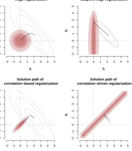
in the parameter space that align with the larger eigendirections of the empirical covari-ance matrix of the regressors. Figure 1 illustrates the solution paths of four different
Solution path of ridge regularization ββ1 ββ2 −2 −1 0 1 2 3 4 5 −2 −1 0 1 2 3 4 5 Solution path of adaptive ridge regularization
ββ1 ββ2 −2 −1 0 1 2 3 4 5 −2 −1 0 1 2 3 4 5 Solution path of correlation−based regularization ββ1 ββ2 −2 −1 0 1 2 3 4 5 −2 −1 0 1 2 3 4 5 Solution path of correlation−driven regularization ββ1 ββ2 −2 −1 0 1 2 3 4 5 −2 −1 0 1 2 3 4 5
Figure 1: Solution paths of four different quadratic penalties for a GLM with Gamma
response, log-link and dispersion parameterφ = 1/2.
quadratic penalties for a GLM with Gamma response, log-link and dispersion parameter
φ= 1/2. The model contains an intercept and two regressors x1 and x2 with correlation
%12 = 0.9, the sample size is n = 30. It is seen that the type of the quadratic penalty
strongly influences the solution path. The ridge penalty in the upper left panel does not give priority to any direction. The adaptive ridge penalty in the upper right panel uses
fixedλ2 = 0.5 yielding strong emphasis on the ordinate. For λ1 → ∞ the component ˆβ2
converges towards 2.671, while ˆβ1 → 0. The correlation-based penalty in the lower left
panel focuses on the bisecting line where its sign is driven by the sign of the correlation between the regressors. The solution path of the correlation-based penalty is similar to that of the ridge penalty with a more strong emphasis on forcing the regressor coeffi-cients to be equal. The correlation-driven penalty (10) (lower right panel) uses weights
We define M∗λ = 0 0>p 0p Mλ , (11)
where0p is the p-dimensional null vector, in order to adjust the dimension of the penalty
matrix to the dimension p+ 1 of the unknown coefficient vector b.
Given a quadratic penalty, the resulting penalized MLE ofbis the solution of the problem
ˆ b= arg min b −`(b) + 1 2b >M∗ λb . (12)
Since the quadratic penalty (6) is twice differentiable, iterative Newton-type methods
can be used to solve (12). Let H denote the Hessian of the log-likelihood (3). Using
F(b) = −IE[H(b)] as an approximation, the update of the penalized Fisher scoring is
b(k+1) = b(k)− F(b(k)) +M∗λ −1 −s(b(k)) +M∗λb(k) = X>W(k)X+M∗λ −1 X>W(k)y˜(k), where W(k) = W(b(k)),D(k) = D(b(k)),µ(k) = h(x>1b(k)), . . . , h(x>nb(k)) >. The
dis-persion parameter φ does not cancel out as in classical Fisher scoring. Since the tuning
parameter λ has been treated as given we simply adjust the penalty matrix Mλ for φ,
e.g. we assume that λ already includes the (unknown) dispersion parameter, and hence
drop it in the estimation equations.
For Mλ = O(p×p) the algorithm coincides with the IRLS algorithm. Hence, penalized
Fisher scoring can be interpreted as a generalization of it. One crucial point for the application is the positive definiteness ofF(b(k)) +M∗λ. AsMλ is assumed to be already
positive definite this condition is fulfilled even for a number of situations wheren p.
The tuning parameterλ, which controls model complexity, must be determined. Consider
for example the ridge penalty (7). When λ = 0 the model includes p+ 1 regression
coefficients which typically are different from zero whereas in the limit λ → ∞ the
intercept β0 is the only nonzero coefficient. If we regard the resulting estimate as a
function ofλ, the number of ‘relevant’ regression coefficients is also a function of λ. The
value of the regularization parameter controls the amount of shrinkageand the amount of
model complexity. Since model complexity of parametric models is related to the number of (regression) parameters it is often expressed in terms of degrees of freedom. In the classical linear model, the degrees of freedom are computed as the trace of the hat matrix. For quadratically penalized GLMs the hat matrix can be derived similar to unpenalized GLMs, see for example Fahrmeir and Tutz (2001). One obtains the form
Hλ = W>/2X(X>WX+M∗λ)−1X>W1/2. (13)
The trace of the hat matrix, df(λ) = tr(Hλ) is used as the degrees of freedom. As
pro-posed by Wood (2006) we estimate the unknown dispersion parameterφby the
Pearson-like dispersion estimator ˆ φ= 1 n−tr(Hλ) n X i=1 (yi−µˆi)2 V(ˆµi) . (14)
However, quadratically penalized MLEs cannot set some components ofb to equal zero. Hence, our idea is to consider a specialized version of componentwise boosting in order to combine improvements by quadratic penalization with variable selection.
4
Forward Boosting
Although they can be used to tailor the shrinkage effect simple quadratically penalized
MLEs do not set components of b to exactly zero. For this reason we will use them in
the following to structure the learner of a specialized boosting method.
Boosting is a successful and flexible strategy which has been originally developed in the machine learning community. A starting point for our investigations has been com-ponentwise boosting that merely improves one selected coefficient within one step, see
for example Friedman et al. (2008), B¨uhlmann and Yu (2006), B¨uhlmann and Hothorn
(2007), and Tutz and Binder (2007). One basic concept in boosting is the use of a weak learner. A weak learner is a fitting procedure that starts from previous estimates and improves the fit only weakly. The final estimate is obtained by applying the stepwise fit repeatedly. In the following we first consider how quadratic penalties work if used directly as a learner and then show how the learner has to be modified to obtain the intended structuring effect.
Consider a structured weak learner that uses a quadratic penalty of the form Pλ(β) =
1
2β>Mλβ, for example the correlation-based penalty (9). Let xA(l) denote a subset of
covariates (including the intercept) that is attained in the l-th iteration of a boosting
algorithm, and γA(l) the corresponding (sub-)vector of coefficients. Boosting improves
the fit within one step by fitting the model
µ=hηˆ(l−1)+x>A(l)γA(l), (15) where the predictor ˆη(l−1) =x>bˆ
(l−1) as estimated from the previous step is treated as an
offset, or more precisely as a fixed constant. The question is how to estimate the update
γA(l) when one wants to account for the assumed association structure as represented in
the quadratic penalty.
As common in componentwise likelihood-based boosting, one might update by
utiliz-ing one-step Fisher scorutiliz-ing with ˆb(l−1) as initial value. Based on the training data set
{(yi,xi)}ni=1 one obtains ˆ γA(l) = (X>A(l)W(ˆη(l−1))XA(l)+M ∗ λ,A(l)) −1X> A(l)D(ˆη (l−1) )Σ−1(ˆη(l−1))(y−µˆ(l−1)), where ˆη(l−1) = (ˆη(1l−1), . . . ,ηˆn(l−1))>, ηˆ(il−1) =x>i bˆ(l−1), µˆ(l−1) ={h(ˆη(1l−1)), . . . , h(ˆη (l−1) n )}>
and M∗λ,A(l) contains the submatrix of M∗λ that corresponds to the indices in A(l). The
main problem with this approach is its restriction to the elements inA(l) and the
conse-quences when the partition M∗λ,A(l) is used instead of the full penalty matrix. Consider
for example the common case of componentwise boosting where|A(l)|= 1 for all l. Then
componentwise ridge boosting, no matter what penalty we have originally chosen. Hence, the assumed association structure will not be taken into account. Alternatively, consider
the application of the correlation-based penalty even when |A(l)| > 1. What happens
when the corresponding elements of M∗
λ are used is that covariates which are strongly
correlated with others are much more penalized then only slightly correlated ones. As a result, the potential update ˆγA(l) is much more closer to zero whenA(l)consists of highly
correlated covariates. This in turn lowers the model fitting ability, and hence reduces the possibility to get chosen for a coefficient update. Consequently, this would facilitate uncorrelated covariates to enter the model much easier than highly correlated ones. But that contradicts the motivation behind the correlation-based penalty.
As a consequence, one has to find a way to incorporate the assumed structure amongall
covariates into the penalty term. One approach to find an appropriate update is ˆ
γ(l)=IA(l)(X>W(ˆη(l−1))X+Mλ∗)−1X>D(ˆη(l−1))Σ−1(ˆη(l−1))(y
−µˆ(l−1)), (16)
where the full vector ˆγ(l) is used and one just selects the elements to be updated with the
diagonal matrixIA(l) where ones are located at the positions corresponding to the elements
of A(l) and zeros elsewhere. Then the whole assumed association structure among all
regressors is regarded, but unfortunately one simply incorporates the association structure left in ˆη(l−1) and ˆµ(l−1), but not the complete structure underlying the original training data. Consequently, using a quadratic penalty solely based on the current update estimate ˆ
γ(l) cannot adjust for the magnitudes of ˆb(l−1). Some evident problems arise e.g. when
we apply the correlation-based penalty. With the current approach it is nearly impossible to gain grouping effects if the variables of one group are not all in or out of the update
set A(l) together. Unfortunately, we seldom a priori know which covariables constitute
a (significant) group. So this must be done adaptively as in the GBlockBoost algorithm (Ulbricht and Tutz, 2008) what in turn can become very time-consuming when there is a large number of covariates.
In the third (and final) approach we will additionally include the previously estimated coefficients ˆb(l−1) in the penalty term. Therefore let us consider the parameter vector
b∗(l)=b(l−1)+γ(l), (17)
where b(l−1) is treated as fixed constant and γ(l) is the unknown update part. The
resulting penalty term is 1 2b ∗> (l)M∗λb∗(l) = 1 2b > (l−1)M∗λb(l−1)+γ>(l)M∗λb(l−1)+ 1 2γ > (l)M∗λγ(l). (18)
Note that this penalty directly incorporates the magnitude of b(l−1). For example, if
one uses the correlation-based penalty then two highly correlated regressors xi and xj
with i ∈ A(l−1), j ∈ A(l), i6= j show comparable absolute values of their corresponding
coefficient estimates inb∗(l), even if A(l−1) and A(l) are disjoint.
As seen from (17), b∗
(l) is composed of two components. Consequently, we need two
γ(l) = 0 as initial values we obtain sp(b∗(l)) = X>D(ˆη(l−1))Σ−1(ˆη(l−1))(y−µˆ(l−1))−M∗λbˆ(l−1) and Fp(b∗(l)) = X>W(ˆη (l−1) )X+M∗λ
for penalized score vector and Fisher information, respectively. The resulting estimate of the update vector is
ˆ
γ(l) =IA(l)F −1
p (b∗(l))sp(b∗(l)). (19)
Here the previous estimate ˆb(l−1) is included in the penalized score vector and hence
modifies the direction of steepest descent in contrast to the update (16).
Through some simple manipulations the update vector ˆγ(l) can be written in a more
tractable form.
Lemma 1. Equation (19) can be written
ˆ γ(l)=IA(l)h(X>Wl−1X+M∗λ)−1X>Wl−1 n D−l−11(y−µˆ(l−1)) + ˆη(l−1)o−bˆ(l−1) i . (20) The proof is given in the Appendix. Note that (20) allows for an interesting interpretation of the update. Indeed, ˆγ(l)swaps the coefficients that correspond with the elements ofA(l)
while all others are maintained. This makes it differ from the usual boosting algorithms such as componentwise boosting, RidgeBoost or GBlockBoost. There the coefficients are successively modified by adding current updates. Here we have a ‘swap or maintain’ strategy.
The resulting boosting algorithm is denoted ForwardBoost and is summarized in the following.
Algorithm Forward Boosting (ForwardBoost)
Step 1: Initialization Fit the model µ = h(β0) by one step of Fisher scoring to
obtain ˆb(0) = ( ˆβ0,0, . . . ,0)> with ˆβ0 = g n1Pni=1yi , and ˆη(0) = Xbˆ(0),µˆ(0) = n h(x>1bˆ(0)), . . . , h(x>nbˆ(0)) o> , Aˆ(0) ={0}.
Step 2: Iteration Forl = 1,2, . . . , lmax
(i) Estimation Consider the potential update set A(l) = A(l−1) ∪ {j}, j ∈
{0,1, . . . , p}. When fitting the model µ=h ηˆ(l−1)+x>γ
(l) use ˆ γ(l) =IA(l)h(X>Wl−1X+M∗λ)−1X>Wl−1 n D−l−11(y−µˆ(l−1)) + ˆη(l−1)o−bˆ(l−1) i .
(ii) Selection Choose the potential update set that improves the fit maximally.
That is
ˆ
A(l) = arg min
A(l)
(iii) Update Forν ∈(0,1] update ˆ b(l) = ˆb(l−1)+νγˆ(l) = ˆb(l−1)+νIAˆ(l) (X>Wl−1X+Mλ∗)−1X>Wl−1× ×nD−l−11(y−µˆ(l−1)) + ˆη(l−1)o−bˆ(l−1) i , where ˆη(l) =Xbˆ(l) and ˆµ(l) = n h(x>1bˆ(l)), . . . , h(x>nbˆ(l)) o> .
Note that the active setA(l) is monotonically increasing. As pointed out the update ˆγ(l)
completely interchanges the corresponding coefficients. Hence, both aspects are similar to the forward selection strategy to obtain suitable subsets of explanatory variables in regression models. For this reason we denote our method as ‘Forward Boosting’.
As mentioned above, the ForwardBoost algorithm can be interpreted as gradient descent algorithm. To prevent from too big movements into a specific direction we use the
additional boosting parameter ν ∈ (0,1]. As a result, the algorithm tends to be more
stable and the occurrence of divergence problems has been reduced. This parameter is not treated directly as a tuning parameter, that is it is not optimized on in a data driven
way. In our experience, using ν = 0.1 is quite a good compromise between increased
stability and an increased number of necessary boosting iterations until convergence.
For ν = 1 the coefficients corresponding to the indices in ˆA(l) are currently updated by
getting replaced by the corresponding elements of ˆγ(l) while all other coefficients remain.
For ν ∈ (0,1) the estimated coefficients ˆb(l) are indeed a convex combination of ˆb(l−1)
and ˆγ(l). This leads to a simple iterative version of the hat matrix.
As we have seen, the initial estimate of b is ˆb(0) = ( ˆβ0,0, . . . ,0)> with ˆβ0 =
g(1/nPni=1yi) yielding an initial hat matrix
Hbˆ(0) =H(0) =
1
n1n1 >
n,
where 1n denotes the n-dimensional vector of ones. In the l-th iteration (l ≥ 1) of the
ForwardBoost algorithm the coefficients update is ˆ b(l) = ˆb(l−1)+νγˆ(l). Let H(l) =Wl>−/12XIAˆ(l)(X >W l−1X+M∗λ)−1X>W 1/2 l−1.
Due to its form the termH(l) is easily seen to be the (generalized) hat matrix of the first
summand on the right hand side of (20). Hence the hat matrix of ˆb(l) is given iteratively
by
We will use the trace ofHˆb(l) as an estimate of degrees of freedom for estimating bin the
l-th boosting iteration. Furthermore we apply the deviance to measure the performance
of potential updates. However, its major problem is that it does not directly penalize for an increasing amount of model complexity when an additional regressor is included. This suggests to rather use an information criterion. Note that we would need to compute the trace of the updated hat matrix in this case. This in turn can become quite time-consuming. When dealing with metric covariates only we are usually on the safe site if we just add one regressor in a single boosting iteration. So the increasing complexity is just one additional parameter and hence can be neglected especially in the longer run when lot of coefficients are already included in the predictor.
Nevertheless, we use information criteria for stopping the algorithm, such as AIC
AIC(ˆb(l)) = Dev(ˆb(l)) + 2 tr(Hˆb(l)), (22)
or BIC
BIC(ˆb(l)) = Dev(ˆb(l)) + log(n) tr(Hbˆ(l)), (23)
where Dev(ˆb(l)) denotes the deviance of the fitted model in thel-th boosting step. Hence
we stop ForwardBoost after the iteration that minimizes the stopping criterion. The trace of the corresponding hat matrix (21) can be used to estimate the unknown dispersion parameter according to (14).
After each iteration we check whether or not there is a definite update in the estimated coefficients. This is measured by
kbˆ(l)−bˆ(l−1)k
kbˆ(l)k
≤ (24)
for some small >0. If not we stop the algorithm. It can happen then that the minimum
position of the stopping criterion coincides with this iteration.
The estimated update set ˆA(l) must be monotonically increasing in l, that is all the
pre-viously updated coefficients must be included in the current active set. This is especially necessary to obtain the grouping effect. For an explanation of the necessity let us
ini-tially consider the monotonically increasing active set ˆA(l). Note that for l → ∞ we
have ˆA(l) → {0,1, . . . , p}. Even if there are some pure noise regressors in the data the
deviance will be improving (at least not getting worse) if some of them are additionally included in the predictor. As a result, in the long run the ForwardBoost algorithm will then tend to include all given regressors in the predictor. However, this will also occur
for componentwise updates but the important point is that in the monotonic case for l
‘large’ the set ˆA(l) will contain all coefficient indices.
Now we look at the resulting estimate of the ForwardBoost algorithm at convergence. We assume that the corresponding penalized Fisher scoring algorithm with identical
M∗λ converges to, say, ˆbQP. The condition of the ForwardBoost algorithm for
conver-gence is that ˆb(l+1) = ˆb(l) (up to small componentwise relative errors). Due to the
M∗λ)−1X>W
l−1
n
D−l−11(y−µˆ(l−1)) + ˆη(l−1)owhat in turn is algebraically equivalent with ˆ
bQP. Note that rather the indexl butW,Dandµmust be identical in ˆb(l−1) and ˆbQP in
order to fulfill the convergence assumption. For this reason both estimates will coincide.
Now consider the set ˆA(l) at convergence again. For monotonic increases this implies
that all elements of ˆb(l−1) and ˆbQP must coincide. If at convergence |Aˆ(l)|< p+ 1 (e.g. |Aˆ(l)| = 1 as for componentwise updates) then it is sufficient for ˆb(l−1) and ˆbQP to just
being equal in the corresponding elements of ˆA(l). Consequently, they do not have to
be equal in all of their elements. Indeed, the monotonic increase of ˆA(l) guarantees the
ForwardBoost algorithm to converge to ˆbQP if it exists. Furthermore, in our experience
using a monotonic increase also fastens the speed of convergence.
We illustrate the functioning of the ForwardBoost algorithm with the following small example. Consider a GLM with Poisson distributed response. The predictor contains an
intercept and three highly correlated regressors x1, x2, x3. The true parameter vector is
b0 = (0.5,1,2,0)>, the correlation structure is %
ij = 0.99|i−j| for i, j = 1,2,3. Due to
this correlation structure the estimated coefficients ˆβ1,βˆ2,βˆ3 are supposed to be nearly
equal if the grouping effect will be gained by the algorithm. We use a sample of size
n= 20. The main results from the first seven iterations are given in Table 1. Note that
the algorithm converges very fast. After seven iterations the change of the estimated
coefficients meets (24) where we have used = 10−8. The resulting coefficient build-up
is visualized in the right panel of Figure 2. In its left panel we visualize the failure of
GBlockBoost in this situation. As you can see the updates ofx2 on one hand andx1 and
x3 on the other behave quite parallel after the second iteration. But the algorithm is not
able to adjust the levels for the coefficients of these both groups.
Another application of the ForwardBoost algorithm is shown in Figure 3. Here we use
a probit model based on n = 75 independent observations. The predictor consists of
an intercept and 11 regressors. The first nine regressors form three clusters of three highly correlated regressors, e.g. x1, x2, x3 are cluster 1, x4, x5, x6 are cluster 2, and
x7, x8, x9 are cluster 3. The clusters are not correlated among themselves. We generate
the correlation%ij among the regressorsxi and xj as%ij =%|i−j|ifi, j belong to the same
cluster, and %ij = 1{i=j} otherwise, that is %ij = 1 if i = j and %ij = 0 otherwise. We
set %= 0.95. The true parameter vector is b0 = (0,1,2,0,1,−2,0,0,0,0,1,0)>. Hence,
the first two clusters are relevant but only the first two components of each cluster are
indeed relevant to predict the response. Furthermore,x10 is also relevant. We have used
Forward Boosting with the correlation-based penalty (9) in the left panel and with the correlation-driven penalty function (10) of the weighted fusion penalty in the right panel. Note that the latter is more adequate in extracting the grouping effect. But we have to find two, instead of one, optimal tuning parameters in this case.
Iteration: l = 1 l = 2 l= 3 l= 4 l= 5 l= 6 l= 7 ˆ γ0(l) −0.00 −0.16 −0.14 −0.05 −0.00 −0.00 −0.00 0.00 0.00 0.00 0.03 0.00 0.00 0.00 0.00 0.11 0.12 0.03 0.00 0.00 0.00 0.00 0.00 0.12 0.03 0.00 0.00 0.00 Dev(ˆγ0 (l)) 185.81 137.38 93.70 62.47 62.43 62.42 62.42 ˆ γ1(l) −0.00 −0.16 −0.14 −0.05 −0.00 −0.00 −0.00 1.14 1.25 1.37 0.03 0.00 0.00 0.00 0.00 0.11 0.12 0.03 0.00 0.00 0.00 0.00 0.00 0.12 0.03 0.00 0.00 0.00 Dev(ˆγ1 (l)) 142.10 99.58 64.41 62.47 62.43 62.42 62.42 ˆ γ2(l) −0.00 −0.16 −0.14 −0.05 −0.00 −0.00 −0.00 0.00 0.00 0.00 0.03 0.00 0.00 0.00 1.14 0.11 0.12 0.03 0.00 0.00 0.00 0.00 0.00 0.12 0.03 0.00 0.00 0.00 Dev(ˆγ2 (l)) 140.09 137.38 93.70 62.47 62.43 62.42 62.42 ˆ γ3(l) −0.00 −0.16 −0.14 −0.05 −0.00 −0.00 −0.00 0.00 0.00 0.00 0.03 0.00 0.00 0.00 0.00 0.11 0.12 0.03 0.00 0.00 0.00 1.14 1.25 0.12 0.03 0.00 0.00 0.00 Dev(ˆγ3 (l)) 140.49 98.31 93.70 62.47 62.43 62.42 62.42
Table 1: The main results for the first 7 iterations of the ForwardBoost algorithm with
λ= 1.5, ν = 1 andPcb
λ (β) as penalty when applied to the Poisson example. We denote the
(potential) updates at thel-th iteration with ˆγr(l) where r indicates the added regressor,
besides the intercept. Consider the first column where l = 1. The intercept has been
already estimated previously. So if β0 is solely to be updated then there is only a small
negative change. As you can see, the grouping effect directly works since all coefficients ˆ
γ11,(1) = ˆγ22,(1) = ˆγ33,(1) = 1.14 get (nearly) identical values. Due to a minimum deviance ˆ
γ2(1) has been chosen for updating, so that ˆβ2,(1) = 1.14. Now consider the second column
wherel = 2. Since ForwardBoost uses monotonic updates,γ2,(2) will always be updated.
As you can see, the grouping effect is also kept here. For the other regressors we get ˆ
γ1,(2) = ˆγ3,(2) = 1.25 which correspond with an update of ˆβ2,(1) about 0.11. Finally, ˆγ3(2)
has been chosen, so that ˆβ2,(2) = ˆβ3,(2) = 1.25. This principle continues in the next
GBlockBoost Iterations Standardiz ed Coefficients 1 2 3 4 5 6 7 8 0 1 2 3 4 ● ● ●x1 x2 x3 ForwardBoost Iterations Standardiz ed Coefficients 1 2 3 4 5 6 7 0.0 0.4 0.8 1.2 ● ● ●x1x2x3 Coefficient build−ups
Figure 2: Coefficient build-up of the GBlockBoost algorithm (Ulbricht and Tutz, 2008)
with λ = 1.5 (left panel) and of the ForwardBoost algorithm with λ = 1.5, ν = 1 and
Pcb
λ (β) as penalty (right panel). Note that the grouping effect of the ForwardBoost
algorithm can be obtained at the earliest after p iterations (here p = 3). This is due to
its construction in the sense of forward selection.
5
Application to Simulations and Real Data
5.1
Simulations
We consider two different classes of simulation settings, a low-dimensional (that isnp)
and a high-dimensional one (n p). In both classes the predictor consists of a number
of blocked regressors and a number of independent regressors.
In the low-dimensional settings we use p= 40 variables, ntrain = 100 training data to fit
the model,nvali = 50 validation data to select optimal tuning parameters and ntest= 50
test data to evaluate the model performances. The true parameters are given by
β0 = (0, . . . ,0 | {z } 10 times ,0.5, . . . ,0.5 | {z } 10 times ,0, . . . ,0 | {z } 10 times ,0.25, . . . ,0.25 | {z } 10 times )
and the true intercept as β0
0 = 0 yieldingb0 = (β00,β0)>. The corresponding covariates
are simulated as multivariate normal random variables with unit variances and the fol-lowing correlation structure: The first 20 covariates constitute two independent blocks of
10 variables each with correlation structure betweenxi and xj
%ij =
%|i−j|, if i, j are in the same block,
1{i=j}, otherwise, (25)
where 1{i=j} = 1 if i = j and 1{i=j} = 0 otherwise. We vary the correlation parameter
Pλλcb ((ββ)) (λλ ==0.001) Number of iterations Coefficients 0 5 10 15 −0.2 0.0 0.2 0.4 0.6 ● ● ● ● ● ● ● ● ● ● ● x1 x2 x3 x4 x5 x6 x7 x8 x9 x10 x11 Pλλwf ((ββ)) (λλ1==0, λλ2==0.1, γγ ==1.5) Number of iterations Coefficients 0 5 10 15 −0.2 0.0 0.2 0.4 0.6 0.8 ●●● ● ● ● ● ● ● ● ● x1 x2 x3 x4 x5 x6 x7 x8 x9 x10 x11
Coefficient build−ups of Forward Boosting with two different penalties
Figure 3: Application of the ForwardBoost algorithm to the simulated probit model. In
the left panel we use the correlation-based penalty (9) withλ= 0.001. In the right panel
we apply the correlation-driven penalty function (10) of the weighted fusion penalty (Daye
and Jeng, 2009) with λ2 = 0.1 and γ = 1.5. Note that λ1 = 0 indicates the irrelevance
of the lasso penalty term, so that variable selection is solely driven by the ForwardBoost
algorithm. When the AIC criterion (22) is used to stop thenl = 9 iterations are optimal
for both penalties.
strength. Note that 0.9910 ≈0.9,0.9510 ≈ 0.6, and 0.510 ≈ 0.001 so that we capture all
three situations of high correlation, mean correlation and nearly no correlation through-out the blocks, respectively. The last 20 covariates are drawn independently from the standard normal distribution. Note that just the second block and the last 10 indepen-dent variables are influential.
In the high-dimensional settings we consider p= 100 regressors and ntrain = 40 training
data for model fitting,nvali = 20 validation data to determine optimal tuning parameters,
and ntest = 20 test data for model evaluation. The true parameters are now given by
β0 = (0, . . . ,0 | {z } 20 times ,0.5, . . . ,0.5 | {z } 10 times ,1, . . . ,1 | {z } 10 times ,0.5, . . . ,0.5 | {z } 10 times ,0.25, . . . ,0.25 | {z } 10 times ,0, . . . ,0 | {z } 40 times ) and again β0
0 = 0 so that b0 = (β00,β0)> as before. Also the correlation structure of
the covariates is similar to the low-dimensional setting. Now the first 50 covariates are blocked into 5 blocks of 10 correlated variables each. The correlation structure is again given by (25). The last 50 covariates are independently drawn from the standard normal distribution. Now just the last three blocks are truly influential as well as the first 10 independent regressors.
For the simulation studies we create 100 replications which are based on the following model assumptions
(i) Logit model with binary dependent observations, i.e. yi ∼ B(1, pi), where pi =
(1 + exp{−ηi})−1;
(ii) a loglinear Poisson model, i.e. yi ∼P ois(λi) with λi = exp{−ηi/4};
In the high-dimensional settings we modify the parameter of model (ii) to λi =
exp{−ηi/24}.
We use the deviance based on the test data as a measure for goodness of fit. For ease of
description we will refer to it asdeviance loss. To consider the explanation ability of our
fitted models, we use
M SEb(ˆb,b0) :=kbˆ−b0k22 (26)
that measures the squared deviation between the estimated coefficients ˆb and the true
parameter vector b0. As the test deviance and M SE
b are based on loss functions, the
smaller their values the better the performance.
Additionally, we use the criteria hits and false positives to evaluate the identification of
relevant regressors. For j = 0,1, . . . , p they are defined as
hits(ˆb,b0) :=n{j : ˆβj 6= 0} ∩ {j :βj0 6= 0}o, (27)
and
f ps(ˆb,b0) :=n{j : ˆβj 6= 0} ∩ {j :βj0 = 0}o, (28)
respectively. Hence, hits refers to the number of correctly identified coefficients, false
positives (f ps) is the number of non-influential regressors (including the intercept if
appropriate) dubbed influential.
We consider the performance of Forward Boosting based on the ridge penalty (FB:ridge), the correlation-based penalty (FB:penalreg), and the weighted-fusion penalty (FB:weighted.fusion), respectively. We compare their results with the performances of lasso, elastic net, RidgeBoost, and GBlockBoost (Ulbricht and Tutz, 2008). For Forward Boosting, the weighted-fusion penalty is reduced to the correlation-driven penalty (10). As proposed by Daye and Jeng (2009) we use
ωij = |
%ij|γ
1− |%ij|
, (29)
whereγ >0 is an additional tuning parameter to compute (10). Note that all considered
methods are invariant towards the order of regressors.
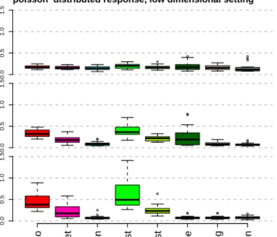
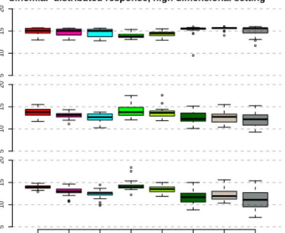
The result for the test deviances and theM SEb are given in Figures 4 to 8. All considered
methods show similar results for the test deviances in all low and high dimensional simulation settings. The level of deviance increases when the correlation among regressors
decreases. However, Forward Boosting shows the best performance in terms of M SEb.
● ρρ == 0.5 10 30 50 70 ● ρρ == 0.95 10 30 50 70 ● ρρ == 0.99 10 30 50 70 lasso enet w eighted.fusion RidgeBoost GBlockBoost FB:r idge FB:penalreg FB:w eighted.fusion De viance loss
binomial distributed response, low dimensional setting
● ● ● ● ● ● ● ● ρρ == 0.5 0 1 2 3 4 5 ● ● ● ● ● ● ρρ == 0.95 0 1 2 3 4 5 ● ● ● ● ● ● ● ● ● ● ● ● ρρ == 0.99 0 1 2 3 4 5 lasso enet w eighted.fusion RidgeBoost GBlockBoost FB:r idge FB:penalreg FB:w eighted.fusion MSE beta
binomial distributed response, low dimensional setting
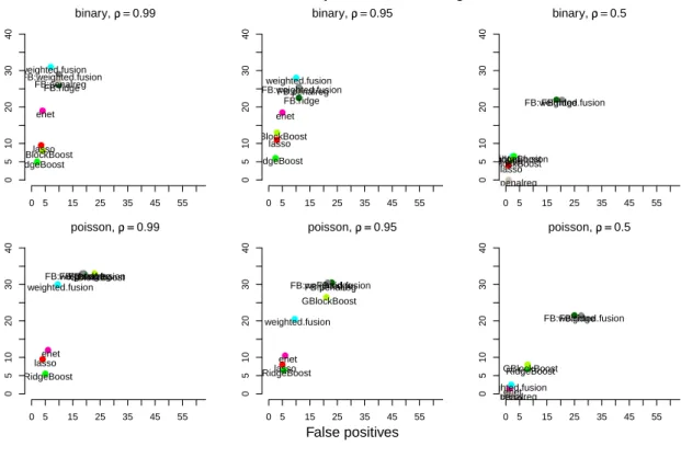
Figure 4: Boxplots of the low dimensional setting with binomial distributed response. RidgeBoost and GBlockBoost, show poor performance in particular when correlation is high. For small correlation the difference between methods is smaller. As is seen from Figures 6 and 9, the ForwardBoost algorithm tends to find the most hits. In the low dimensional settings all methods, besides GBlockBoost, behave quite similar in the number of false positives. In the high dimensional settings this aspect slightly changes
as the ForwardBoost tends to select some more false positives especially when % = 0.5.
However, this primarily refers to the inclusion of the grouping effect.
5.2
Predicting Fat Content From Spectrometric Wavelengths
Chemometrics deals with the data-driven extraction of information from chemical sys-tems. One important field is signal regression where the outcomes are scalars and the regressors are one-dimensional signals that have been measured by some (near infrared) spectroscopy analysis. A nice overview on statistical tools for signal regression has been given by Frank and Friedman (1993). Applications in signal regression are usually
charac-terized by high correlations between neighboring regressors and annpdata situation.
Signal regression is often related to functional data analysis (Ramsay and Silverman, 2005). The latter interprets the regressors as smooth function.
If the main concern of data analysis is prediction, then smoothing of regressors might be appropriate. On the other hand, regressor selection is of interest from the viewpoint of interpretability. One wants to know which covariates effect upon the response. For spectroscopy data we are primarily interested in finding relevant areas of wavelengths (Tutz and Gertheiss, 2010). As common techniques of functional regression analysis are not capable of this we will focus on shrinkage and boosting methods in the following.
● ● ρρ == 0.5 20 40 60 80 100 ● ρρ == 0.95 20 40 60 80 100 ● ρρ == 0.99 20 40 60 80 100 lasso enet w eighted.fusion RidgeBoost GBlockBoost FB:r idge FB:penalreg FB:w eighted.fusion De viance loss
poisson distributed response, low dimensional setting
● ● ● ● ● ρρ == 0.5 0.0 0.5 1.0 1.5 ● ● ● ● ● ● ρρ == 0.95 0.0 0.5 1.0 1.5 ● ● ● ● ● ●● ● ρρ == 0.99 0.0 0.5 1.0 1.5 lasso enet w eighted.fusion RidgeBoost GBlockBoost FB:r idge FB:penalreg FB:w eighted.fusion MSE beta
poisson distributed response, low dimensional setting
Figure 5: Boxplots of the low dimensional setting with Poisson distributed response.
● ●● ● ●●●● binary, ρρ ==0.99 0 5 10 15 20 0 5 10 15 20 lasso enet weighted.fusion RidgeBoost GBlockBoostFB:penalregFB:ridge FB:weighted.fusion ● ● ● ● ● ●●● binary, ρρ ==0.95 0 5 10 15 20 0 5 10 15 20 lasso enet weighted.fusion RidgeBoost GBlockBoost FB:ridge FB:penalreg FB:weighted.fusion ●● ● ●● ● ● ● binary, ρρ ==0.5 0 5 10 15 20 0 5 10 15 20 lassoenet weighted.fusion RidgeBoostGBlockBoost FB:ridge FB:penalreg FB:weighted.fusion ● ● ● ● ● ● ● ● poisson, ρρ ==0.99 0 5 10 15 20 0 5 10 15 20 lasso enet weighted.fusion RidgeBoost GBlockBoost FB:ridge FB:penalreg FB:weighted.fusion ● ● ● ● ● ● ● ● poisson, ρρ ==0.95 0 5 10 15 20 0 5 10 15 20 lasso enet weighted.fusion RidgeBoost GBlockBoost FB:ridge FB:penalreg FB:weighted.fusion ● ●●● ● ● ● ● poisson, ρρ ==0.5 0 5 10 15 20 0 5 10 15 20 lasso enet weighted.fusionRidgeBoost GBlockBoost FB:ridge FB:penalreg FB:weighted.fusion False positives Hits
Hits vs. false positives, LD settings
● ● ● ● ● ● ● ● ● ● ● ● ρρ == 0.5 0 10 20 30 40 ● ● ● ● ● ● ● ● ρρ == 0.95 0 10 20 30 40 ● ● ● ● ● ρρ == 0.99 0 10 20 30 40 lasso enet w eighted.fusion RidgeBoost GBlockBoost FB:r idge FB:penalreg FB:w eighted.fusion De viance loss
binomial distributed response, high dimensional setting
● ● ● ● ● ● ● ● ● ● ● ρρ == 0.5 5 10 15 20 ● ● ● ρρ == 0.95 5 10 15 20 ● ● ● ● ● ● ● ● ● ● ● ρρ == 0.99 5 10 15 20 lasso enet w eighted.fusion RidgeBoost GBlockBoost FB:r idge FB:penalreg FB:w eighted.fusion MSE beta
binomial distributed response, high dimensional setting
Figure 7: Boxplots of the high dimensional setting with binomial distributed response.
● ● ● ● ● ● ● ρρ == 0.5 10 30 50 70 ● ● ● ● ● ● ● ● ● ● ● ● ρρ == 0.95 10 30 50 70 ● ● ● ● ● ● ● ● ● ρρ == 0.99 10 30 50 70 lasso enet w eighted.fusion RidgeBoost GBlockBoost FB:r idge FB:penalreg FB:w eighted.fusion De viance loss
poisson distributed response, high dimensional setting
● ● ● ρρ == 0.5 0.0 0.4 0.8 ● ● ● ● ● ρρ == 0.95 0.0 0.4 0.8 ● ● ● ● ● ● ρρ == 0.99 0.0 0.4 0.8 lasso enet w eighted.fusion RidgeBoost GBlockBoost FB:r idge FB:penalreg FB:w eighted.fusion MSE beta
poisson distributed response, high dimensional setting
● ● ● ● ● ● ●● binary, ρρ ==0.99 0 5 15 25 35 45 55 0 5 10 20 30 40 lasso enet weighted.fusion RidgeBoost GBlockBoost FB:ridge FB:penalreg FB:weighted.fusion ● ● ● ● ● ● ● ● binary, ρρ ==0.95 0 5 15 25 35 45 55 0 5 10 20 30 40 lasso enet weighted.fusion RidgeBoost GBlockBoost FB:ridge FB:penalreg FB:weighted.fusion ●● ●● ● ● ● ● binary, ρρ ==0.5 0 5 15 25 35 45 55 0 5 10 20 30 40 lassoenet weighted.fusionGBlockBoostRidgeBoost
FB:ridge FB:penalreg FB:weighted.fusion ● ● ● ● ● ● ● ● poisson, ρρ ==0.99 0 5 15 25 35 45 55 0 5 10 20 30 40 lasso enet weighted.fusion RidgeBoost GBlockBoost FB:ridge FB:penalreg FB:weighted.fusion ● ● ● ● ● ● ● ● poisson, ρρ ==0.95 0 5 15 25 35 45 55 0 5 10 20 30 40 lasso enet weighted.fusion RidgeBoost GBlockBoost FB:ridge FB:penalreg FB:weighted.fusion ●● ● ● ● ● ● ● poisson, ρρ ==0.5 0 5 15 25 35 45 55 0 5 10 20 30 40 lassoenet weighted.fusion RidgeBoost GBlockBoost FB:ridge FB:penalreg FB:weighted.fusion False positives Hits
Hits vs. false positives, HD settings
Figure 9: Hits versus false positives, high dimensional (HD) settings
The original data we want to analyze come from a quality control problem in food industry
and has been used in Ferraty and Vieu (2006). This data set concerns a sample ofn = 215
pieces of finely chopped meat. The response is the content of fat, the regressors consist
of a channel spectrum of absorbances that has been discretized to p = 100 equidistant
points. These data have been recorded on a Tecator Infratec Food and Feed Analyzer working in the wavelength range from 850 to 1050 nm by the Near Infrared Transmission (NIT) principle. Given a new set of spectrometric wavelengths the task is to predict the corresponding fat content. Indeed, it is less expensive (in terms of time and costs) to obtain the spectrometric wavelengths than to determine the percentage of fat. Hence, it is an important challenge to predict the fat content from the spectrometric data.
We randomly split the data set intontrain = 129 training data to fit the model,nvali = 43
validation data to determine the tuning parameters with the help of the AIC criterion,
and ntest= 43 test data to evaluate model performance. We repeat the random splitting
20 times. In order to apply a GLM we need to specify the exponential family of the response and a suitable link function in a first step. The model specification that has clearly ruled out the other competing ones was the inverse Gaussian distribution with log-link. As there is a natural order between the wavelengths we additionally consider the fused lasso penalty (Tibshirani et al., 2005) in the following.
lasso 850 900 950 1000 1050 −10 0 5 10 enet 850 900 950 1000 1050 −5 0 5 fused.lasso 850 900 950 1000 1050 −0.5 0.5 1.5 weighted.fusion 850 900 950 1000 1050 −0.5 0.0 0.5 1.0 RidgeBoost 850 900 950 1000 1050 −1 0 1 2 3 GBlockBoost 850 900 950 1000 1050 −1 1 2 3 4 5 FB:weighted.fusion 850 900 950 1000 1050 0.00 0.05 0.10 0.15 FB:ridge 850 900 950 1000 1050 −0.4 0.0 0.4 0.8 FB:penalreg 850 900 950 1000 1050 0.00 0.04 0.08 0.12 wavelength Estimated coefficients
Estimated Coefficients for Chemometric Data
Figure 10: Estimated regressor coefficients for the chemometric data set. To help you identify the single replications we use a color spectrum from red (first replication) to blue (last replication).
Figure 10 shows the estimated regressor coefficients of all 20 replications. Forward Boost-ing shows the best results with regard to the combination of sparsity and smoothness. While lasso, elastic net, RidgeBoost and GBlockBoost tend to favor regression models which are too sparse, fused lasso and weighted fusion select models with high complexity. Furthermore the two latter methods show quite instable results through the 20 replica-tions. Variable selection for Forward Boosting is very stable. The ridge penalty again tends to models which are too sparse not considering any groupings.
6
Conclusion
We proposed a new boosting technique that combines quadratic penalization and explicit variable selection in GLMs. As the monotonically increasing set of active regressors and the structure of the weak learner are quite similar to forward selection in classical regression models we denote our method as Forward Boosting. It has turned out to be highly competitive in both simulation studies and application to real data, especially when the focus is more on identifying the true model than on gaining perfect prediction. Hence, our new method is primarily intended when to study the association structure
between regressors and their relations to the response.
The ForwardBoost algorithm is quite competitive even from computational complexity. The monotonicity of the active regressor set encourages an increase in speed of
conver-gence. This still holds for ν < 1. In our experience, the algorithm behaves very stable.
We have seen that the choice of a concrete quadratic penalty does not matter much in performance. Consequently, quadratic penalties with a single tuning parameter, such as the correlation-based penalty, might be favored, especially when another focus is on the incorporation of grouping effects.
Appendix
Proof of Lemma 1:
To simplify notation we use Wl−1 =W(ˆη(l−1)),Σl−1 =Σ(ˆη(l−1)) and Dl−1 =D(ˆη(l−1)).
It holds that (X>Wl−1X+Mλ∗)−1X>Wl−1X−I = (X>Wl−1X+Mλ∗)−1X>Wl−1X −(X>Wl−1X+M∗λ)−1(X>Wl−1X+M∗λ) = −(X>Wl−1X+M∗λ)−1M∗λ, (30) so we could write ˆ γ(l) = IAl(X >W l−1X+M∗λ)−1 n X>Dl−1Σ−l−11(y−µˆ (l−1) )−M∗λbˆ(l−1) o = IAln(X>Wl−1X+M∗λ)−1X>Dl−1Σ−l−11(y−µˆ(l−1))− −(X>Wl−1X+Mλ∗)−1M∗λbˆ(l−1) o (30) = IAln(X>Wl−1X+M∗λ)−1X>Dl−1Σ−l−11(y−µˆ(l−1))+ + (X>Wl−1X+M∗λ)−1X>Wl−1Xbˆ(l−1)−bˆ(l−1) o = IAl h (X>Wl−1X+M∗λ)−1 n X>Dl−1Σ−l−11(y−µˆ (l−1) )+ +X>Wl−1Xbˆ(l−1) o −bˆ(l−1) i .
Since Dl−1Σ−l−11 =Wl−1D−l−11 and Xbˆ(l−1) = ˆη(l−1) the proposed result follows.
References
B¨uhlmann, P. and T. Hothorn (2007). Boosting algorithms: Regularization, prediction
and model fitting. Statistical Science 22(4), 477–505.
B¨uhlmann, P. and B. Yu (2006). Sparse boosting. Journal of Machine Learning
Daye, Z. J. and X. J. Jeng (2009). Shrinkage and model selection with correlated variables
via weighted fusion. Computational Statistics and Data Analysis 53, 1284–1298.
Fahrmeir, L. and G. Tutz (2001). Multivariate Statistical Modelling based on Generalized
Linear Models (2nd ed.). New York: Springer.
Ferraty, F. and P. Vieu (2006). Nonparametric Functional Data Analysis: Theory and
Practice. New York: Springer.
Frank, I. E. and J. H. Friedman (1993). A statistical view of some chemometrics regression
tools (with discussion). Technometrics 35, 109–148.
Friedman, J., T. Hastie, and R. Tibshirani (2008). Regularization paths for general-ized linear models via coordinate descent. Technical report, Department of Statistics, Stanford University, Stanford.
Nelder, J. A. and R. W. M. Wedderburn (1972). Generalized linear models. Journal of
the Royal Statistical Society, Series A 135, 370–384.
Ramsay, J. O. and B. W. Silverman (2005). Functional Data Analysis (2nd ed.). New
York: Springer.
Slawski, M., W. zu Castell, and G. Tutz (2009). Feature selection guided by structural information. Technical Report 051, Department of Statistics, University of Munich.
Tibshirani, R. (1996). Regression shrinkage and selection via the lasso. Journal of the
Royal Statistical Society B 58, 267–288.
Tibshirani, R., M. Saunders, S. Rosset, J. Zhu, and K. Knight (2005). Sparsity and
smoothness via the fused lasso. Journal of the Royal Statistical Society B 67, 91–108.
Tutz, G. and H. Binder (2007). Boosting ridge regression. Computational Statistics &
Data Analysis 51, 6044–6059.
Tutz, G. and J. Gertheiss (2010). Feature extraction in signal regression: A boosting
technique for functional data regression. Journal of Computational and Graphical
Statistics 19, 154–174.
Tutz, G. and J. Ulbricht (2009). Penalized regression with correlation based penalty. Statistics and Computing 19, 239–253.
Ulbricht, J. and G. Tutz (2008). Boosting correlation based penalization in generalized
linear models. In Shalabh and C. Heumann (Eds.), Recent Advances in Linear Models
and Related Areas. Heidelberg: Springer.
Wood, S. N. (2006). Generalized Additive Models: An Introduction with R. Boca Raton:
Yuan, M. and Y. Lin (2006). Model selection and estimation in regression with grouped
variables. Journal of the Royal Statistical Society B 68, 49–67.
Zou, H. and T. Hastie (2005). Regularization and variable selection via the elastic net. Journal of the Royal Statistical Society B 67, 301–320.