Exploring link, text and spatial-temporal data in social media

(1)

c

(2)

EXPLORING LINK, TEXT AND SPATIAL-TEMPORAL DATA IN SOCIAL MEDIA

BY ZHIJUN YIN

DISSERTATION

Submitted in partial fulfillment of the requirements for the degree of Doctor of Philosophy in Computer Science

in the Graduate College of the

University of Illinois at Urbana-Champaign, 2012

Urbana, Illinois

Doctoral Committee:

Professor Jiawei Han, Chair & Director of Research Associate Professor Chengxiang Zhai

Professor Thomas S. Huang

(3)

Abstract

With the development of Web 2.0, a huge amount of user generated data in social media sites is attracting the attentions from different research areas. Social media data has heterogenous data types including link, text and spatial-temporal information, which poses many inter-esting and challenging tasks for data mining. Link is the representation of the relationships in social networking sites. Text data includes user profiles, status updates, posted articles, social tags, etc. Mobile applications make spatial-temporal information widely available in social media. The objective of my thesis is to advance the data mining techniques in the social media setting. Specifically I will mine useful knowledge from social media by taking advantage of the heterogenous information including link, text and spatial-temporal data. First, I propose a link recommendation framework to enhance the link structure inside so-cial media. Second, I use the text and spatial information to mine geographical topics from social media. Third, I utilize the text and temporal information to discover periodic topics from social media. Fourth, I take advantage of both link and text information to detect community-based topics by incorporating community discovery into topic modeling. Last, I aggregate the spatial-temporal information from geo-tagged social media and mine inter-esting trajectories. All of my studies integrate the link, text and spatial-temporal data from different perspectives, which provide advanced principles and novel methodologies for data mining in social media.

(4)

(5)

Acknowledgments

I would like to thank all the people who have helped me during my Ph.D. study in the past several years.

First and foremost, I would like to express my deepest gratitude to my advisor Professor Jiawei Han for his help throughout my Ph.D. study. His vision, patience, enthusiasm and encouragement inspire me to think deeply and do solid work. This thesis would not have been possible without his support.

Also I would like to thank other doctoral committee members, Professor Chengxiang Zhai, Professor Thomas Huang and Professor Jiebo Luo, for their invaluable help on my research and constructive suggestions on the dissertation.

During my Ph.D. study, it is my great honor to work with talented colleagues in Data Mining group and Database and Information System (DAIS) group. I owe sincere gratitude to my collaborators, especially, Liangliang Cao, Manish Gupta, Xin Jin, Rui Li, Xiaolei Li, Yizhou Sun, Tim Weninger, Qiaozhu Mei. I also thank all the current and former Data Mining group-mates Deng Cai, Chen Chen, Hong Cheng, Marina Danilevsky, Hongbo Deng, Bolin Ding, Jing Gao, Hector Gonzalez, Quanquan Gu, Ming Ji, Hyung Sul Kim, Sangkyum Kim, Jae-Gil Lee, Zhenhui Li, Xide Lin, Jialu Liu, Lu-An Tang, Chi Wang, Jingjing Wang, Tianyi Wu, Dong Xin, Xiao Yu, Bo Zhao, Peixiang Zhao, Feida Zhu.

Last but not least, I am indebted to my wife Weiyi Zhou and my family for their love all the time.

(6)

List of Tables

3.1 Attributes and relationships of users in a social network. . . 16

3.2 Statistics of datasets. . . 22

3.3 Comparison of the methods in DBLP dataset. . . 26

3.4 Comparison of the methods in IMDB dataset. . . 27

3.5 Recommended Persons in DBLP dataset. . . 29

3.6 Attribute Ranking in DBLP dataset. . . 30

4.1 Notations used in problem formulation. . . 34

4.2 Notations used in LGTA framework. . . 38

4.4 Topics discovered in Landscape dataset. . . 47

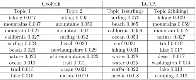
4.5 Topics discovered in Activity dataset. . . 49

4.6 Topic Southbysouthwest in Festival dataset. . . 50

4.7 Topic Acadia in National park dataset. . . 51

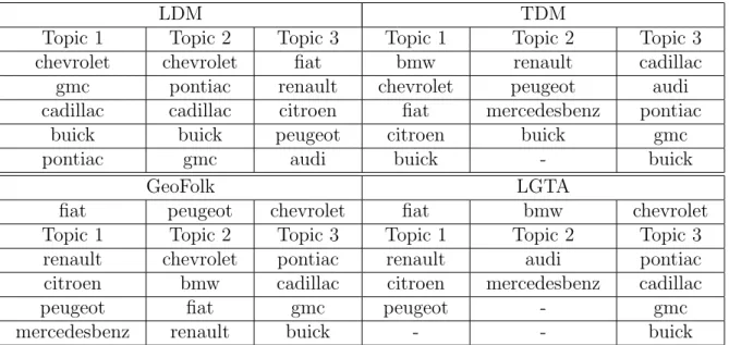
4.8 Topics discovered in Car dataset. . . 52

4.9 Text perplexity in datasets. . . 53

4.10 Location and text perplexity in datasets. . . 54

4.11 Average KL-divergence between topics in datasets. . . 54

4.12 Topics discovered in Food dataset. . . 56

5.2 Selected periodic topics by LPTA. . . 70

5.3 Selected topics by PLSA and LDA. . . 74

5.4 Periodic topics in SIGMOD vs. VLDB and SIGMOD vs. CVPR datasets. . . 75

5.5 Topics in periodic vs. bursty dataset by LPTA. . . 76

5.6 Accuracy and NMI in datasets. . . 79

6.2 Topics in DBLP dataset by LCTA. . . 93

6.3 Selected communities in DBLP dataset by LCTA. . . 94

6.4 Topics in Twitter dataset by LCTA. . . 95

6.5 Selected communities in Twitter dataset by LCTA. . . 96

6.6 Topics in DBLP dataset by NormCut+PLSA. . . 98

6.7 Topics in DBLP dataset by SSNLDA+PLSA. . . 98

(10)

6.9 Accuracy and NMI by NormCut, SSNLDA and LCTA. . . 100

6.10 Accuracy and NMI by PLSA, NetPLSA, LinkLDA and LCTA. . . 101

6.11 Normalized cut in DBLP dataset by PLSA, NetPLSA, LinkLDA and LCTA. 102 6.12 Normalized cut in Twitter dataset by PLSA, NetPLSA, LinkLDA and LCTA. 102 6.13 Communities when the number of communities is 4. . . 103

6.14 Selected communities when the number of communities is 20. . . 104

6.15 Selected topics in DBLP dataset when the number of topics is 20. . . 105

7.1 Top locations in London and their descriptions. . . 111

7.2 An example of sequential pattern mining. . . 112

7.3 Top frequent trajectory patterns in London. . . 113

7.4 A toy example of trajectory pattern ranking. . . 116

7.5 Top ranked trajectory patterns in London. . . 117

7.6 Top ranked locations in London with normalized PL scores. . . 118

7.7 Diversification of trajectory patterns in London. . . 121

(11)

List of Figures

3.1 An augmented graph with person and attribute nodes. . . 16

3.2 Verification of link recommendation criteria in datasets. . . 23

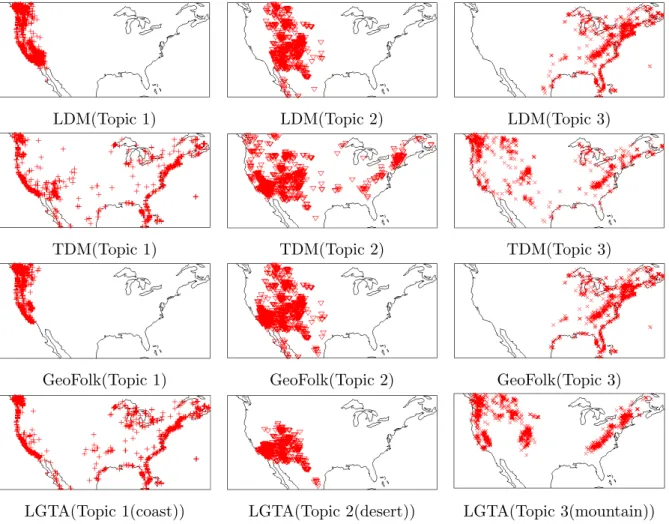
4.1 Document locations of topics in Landscape dataset. . . 48

4.2 Topic comparison in Car dataset. . . 55

4.3 Topic comparison in Food dataset. . . 57

5.1 Timestamp distribution for the topic related to Coachella festival. . . 61

5.2 Timestamp distributions of topic VLDB and its words. . . 72

7.1 Relationship among user, location and trajectory in geo-tagged social media. 114 7.2 Comparison of NDCG@10. . . 124

7.3 Comparison of Location coverage. . . 125

7.4 Comparison of trajectory coverage. . . 125

(12)

Chapter 1 Introduction

The phenomenal success of social media sites, such as Facebook, Twitter, LinkedIn and Flickr, has revolutionized the way of people to communicate and think. This paradigm has attracted the attention of researchers that wish to study the corresponding social and technological problems. A huge amount of data is generated from these social media sites and it incorporates rich information that has rarely been studied in the setting of social media before. Unlike traditional datasets, social media data has heterogenous data types including link, text and spatial-temporal information. New methodologies are urgently needed for data analysis and many potential applications in social media. My thesis focuses on exploring the techniques to mine the knowledge from social media by taking advantage of embedded heterogenous information.

Social media contains three interesting dimensions including link, text and spatial-temporal data. First, link is the key concept underlying the social networking sites. Facebook considers links as undirected friendships, while LinkedIn highlights links as colleagues and classmates. Twitter uses the follower-followee relationships, which are directed links. Link is not only the representation of pair-wise relationship but also an important indication for social influence and community behavior. Second, text exists everywhere in social media. Users describe their hobbies and backgrounds in their profiles, update their status and write or share in-teresting articles. They also use text to tag objects like images and videos and post their corresponding comments. Third, spatial-temporal information is embedded in social media. Some sites record the timestamps of user actions and obtain the geographical information through mobile applications. These spatial-temporal features can help us discover common

(13)

wisdoms and analyze user behaviors.

In this thesis I explore the heterogenous data types in social media including link, text and spatial-temporal information and mine useful knowledge. First, considering the importance of links, I propose a link recommendation framework to enhance the link structure inside social media [109, 110]. Second, we propose a Latent Geographical Topic Analysis framework to mine geographical topics in social media by utilizing the text and spatial information [108]. Third, we propose a Latent Periodic Topic Analysis framework to discover periodic topics in social media by exploiting the periodicity of the terms as well as term co-occurrences [106]. Fourth, we propose a Latent Community Topic Analysis framework to discover community-based topics in social media by incorporating community discovery into topic modeling. Last, we aggregate the spatial-temporal information from geo-tagged social media and mined interesting trajectory patterns [107]. All these studies integrate the link, text and spatial-temporal information in social media from different perspectives and provide new principles and novel methodologies for data mining in social media using heterogenous dimensions. The studies in my thesis are summarized as follows.

• Link Recommendation Link recommendation is a critical task that not only helps increase the linkage inside the network and also improves user experience. In an effective link recommendation algorithm it is essential to identify the factors that influence link creation. Our study enumerates several of these intuitive criteria and proposes an approach that satisfies these factors. Our approach estimates link relevance by using random walk algorithm on an augmented social graph with both attribute and structure information. The global and local influences of the attributes are leveraged in the framework as well. Other than link recommendation, our framework can also rank the attributes in the network. Experiments on DBLP and IMDB data sets demonstrate that our method outperformed state-of-the-art methods for link recommendation. • Latent Geographical Topic Analysis We study the problem of discovering and

(14)

compar-ing geographical topics from GPS-associated documents. GPS-associated documents become popular with the pervasiveness of location-acquisition technologies. For exam-ple, in Flickr, the geo-tagged photos are associated with tags and GPS locations. In Twitter, the locations of the tweets can be identified by the GPS locations from smart phones. Many interesting concepts, including cultures, scenes, and product sales, cor-respond to specialized geographical distributions. We are interested in two questions: (1) how to discover different topics of interests that are coherent in geographical re-gions? (2) how to compare several topics across different geographical locations? To answer these questions, we propose and compare three ways of modeling geographical topics: location-driven model, text-driven model, and a novel joint model called LGTA (Latent Geographical Topic Analysis) that combines location and text. We show that LGTA works well at not only finding regions of interests but also providing effective comparisons of the topics across different locations. The results confirm our hypothe-sis that the geographical distributions can help modeling topics, while topics provide important clues to group different geographical regions.

• Latent Periodic Topic Analysis We study the problem of latent periodic topic analysis from timestamped documents. The examples of timestamped documents include news articles, sales records, financial reports, TV programs, and more recently, posts from social media websites such as Flickr, Twitter, and Facebook. Different from detecting periodic patterns in traditional time series database, we discover the topics of coherent semantics and periodic characteristics where a topic is represented by a distribution of words. We propose a model called LPTA (Latent Periodic Topic Analysis) that exploits the periodicity of the terms as well as term co-occurrences. To show the effectiveness of our model, we collect several representative datasets including Seminar, DBLP and Flickr. The results show that our model can discover the latent periodic topics effectively and leverage the information from both text and time well.

(15)

• Latent Community Topic Analysis We study the problem of latent community topic analysis in text-associated graphs. With the development of social media, a lot of user-generated content is available with user networks. Along with rich information in networks, user graphs can be extended with text information associated with nodes. Topic modeling is a classic problem in text mining and it is interesting to discover the latent topics in text-associated graphs. Different from traditional topic modeling methods considering links, we incorporate community discovery into topic analysis in text-associated graphs to guarantee the topical coherence in the communities so that users in the same community are closely linked to each other and share common latent topics. We handle topic modeling and community discovery in the same framework. In our model we separate the concepts of community and topic, so one community can correspond to multiple topics and multiple communities can share the same topic. We compare different methods and perform extensive experiments on two real datasets. The results confirm our hypothesis that topics help understand community structure, while community structure helps model topics.

• Trajectory Pattern Ranking Social media including those popular photo sharing web-sites is attracting increasing attention in recent years. As a type of user-generated data, wisdom of the crowd is embedded inside such social media. In particular, millions of users upload to Flickr their photos, many associated with temporal and geographical information. We study how to rank the trajectory patterns mined from the uploaded photos with geotags and timestamps. The main objective of our study is to reveal the collective wisdom in the seemingly isolated photos and mine the travel sequences reflected by the geo-tagged photos. Instead of focusing on mining frequent trajectory patterns from geo-tagged social media, we put more effort into ranking the mined trajectory patterns and diversifying the ranking results. Through leveraging the rela-tionships among users, locations and trajectories, we rank the trajectory patterns. We

(16)

then use an exemplar-based algorithm to diversify the results in order to discover the representative ones. We evaluate the proposed framework on 12 different cities using a Flickr dataset and demonstrate its effectiveness.

The remainder of the thesis is organized as follows. Chapter 2 provides an overview of the related work. In Chapter 3, 4, 5, 6 and 7 present our studies for link recommendation, latent geographical topic analysis, latent periodic topic analysis, latent community topic analysis and trajectory pattern ranking in social media respectively. Chapter 8 summarizes the thesis.

(17)

Chapter 2 Related Work

In this chapter we review the related work. In this thesis we would like to explore link, text and spatial-temporal data in social media, so we survey the existing literature on link mining, text mining and spatial-temporal mining in social media in the following sections.

2.1 Link Mining in Social Media

In [33, 34], Getoor et al. classified link mining tasks into three types: object-related, link-related, and graph-related. Object-related tasks include object ranking, object classification, cluster analysis and record linkage or object identification. Link-related tasks include iden-tifying link type, predicting link strength and predicting link cardinality. Graph-related tasks include subgraph discovery, graph classification and generative models for graphs. In this section, we mainly focus on the related link mining tasks including link prediction and community discovery.

Link prediction Link prediction methods include node similarity based, topological ptern based and probabilistic inference based methods. Node similarity based methods at-tempt to seek an appropriate distance measure for two objects. In [24], Debnath et al. estimated the weight values from a set of linear regression equations obtained from a social network graph that captures human judgement about similarity of items. Kashima et al. [48] used node information for link prediction on metabolic pathway, protein-protein interaction and coauthorship datasets. They used label propagation over pairs of nodes with multiple link types and predict relationships among the nodes. Topological pattern based methods

(18)

focus on exploiting either local or global patterns that could well describe the network. In [15], Chen et al. presented a data clustering algorithm K-destinations using random walk hitting time on directed graphs. In [29], the authors used random-walk related measures like square root of the average commute time and the pseudo-inverse of the Laplacian matrix to compute similarity between nodes. In [60], Nowell and Kleinberg suggested that link predic-tions could be done using network topology alone. They presented results on coauthorship networks using features like common neighbors, Jaccard’s coefficient, Adamic/Adar, prefer-ential attachment, hitting time, commute time, and SimRank. In [61], they also suggested using meta-approaches like low rank approximation, unseen bi-grams and clustering besides the above features. Probabilistic inference can also help capture the correlations among the links [47, 52, 89, 96]. Some studies have combined the above mentioned approaches. Hasan et al. [41] identified a mix of node and graph structure features for supervised learning us-ing SVMs, decision trees and multilayer perceptrons to predict coauthorship relationships. In [76], Madadhain et al. learned classifiers like logistic regression and naive bayes for pre-dicting temporal link using both network and the entity features. In [83], Popescul and Ungar proposed the usage of statistical relational learning to build link prediction models. In [85], Rattigan and Jensen demonstrated the effectiveness of link prediction models to solve the problem of anomalous link discovery.

Community discovery Community discovery, a.k.a. group detection [34], is to divide the network nodes into densely connected subgroups [74, 73, 19, 77, 57], which is an important task in datasets including social networks [78], web graphs [28], biological networks [37], co-authorship networks [72], etc. Tang et al. [95] provided a good overview of community discovery algorithms using network structures. Newman et al. [74] proposed an algorithm to remove edges from the network iteratively to split it into communities. The edges removed being identified using betweenness measures and the measures are recalculated after each removal. Palla et al. [77] analyzed the statistical features of overlapping communities to un-cover the modular structure of complex systems. In [87], Ruan et al. introduced an efficient

(19)

spectral algorithm for modularity optimization to discover community structure. Nowicki et al. [75] proposed a statistical approach to a posteriori blockmodeling to partition the ver-tices of the graph into several latent classes where the probability distribution of the relation between two vertices depends only on the classes to which they belong. In [113], Zhang et al. proposed an LDA-based hierarchical Bayesian algorithm called SSN-LDA, where commu-nities are modeled as latent variables in the graphical models and defined as distributions over social actor space. In [112], Zhang et al. used a Gaussian distribution with inverse-Wishart prior to model the arbitrary weights that are associated with the social interaction occurrences. Leskovec et al. [57] studied a range of network community detection methods originating from theoretical computer science, scientific computing, and statistical physics in order to compare them and to understand their relative performance and the systematic biases in the clusters they identify. Yang et al. [120] proposed a graph clustering algorithm (similar to k-medoids) based on both structural and attribute similarities through a unified distance measure. In [63], Long et al. proposed a probabilistic model for relational clustering under a large number of exponential family distributions.

2.2 Text Mining in Social Media

In this section we provide an overview of the related work to text mining in social media. We review the existing studies on topic modeling and the extension with link and spatial-temporal information. We also survey the work related to event detection and tracking.

Topic modeling Statistical topic models can be considered as the probabilistic models for uncovering the underlying semantic structure of a document collection based on hierarchical Bayesian analysis of the text collection. Topic models, such as PLSA [44] and LDA [9], use a multinomial word distribution to represent a semantic coherent topic and model the gen-eration of the text collection with a mixture of such topics. There are also many extensions of the traditional topic models [6, 7, 8, 58].

(20)

Topic modeling with links Some studies extended topic modeling with links. In [68], Mei et al. introduced a model called NetPLSA that regularizes a statistical topic model with a harmonic regularizer based on a graph structure in the data. In [94], Sun et al. defined a multivariate Markov Random Field for topic distribution random variables for each document to model the dependency relationships among documents over the network structure. Zhou et al. [119] proposed a generative probabilistic model to discover semantic community in social networks, but they used text information only without considering link structure. There are several studies on generative topic models based on text and links including Author-Topic model [93, 86], Author-Recipient-Topic model [66, 67, 79], Group-Topic model [103], Link-PLSA-LDA [71], Block-LDA [3], Topics-on-Participations model [115, 116]. The generation of each link in a document is modeled as a sampling from a topic-specific distribution over documents [20, 26]. Liu et al. [62] proposed a model called Topic-Link LDA where the membership of authors is modeled with a mixture model and whether a link exists between two documents follows a binomial distribution parameterized by the similarity between topic mixtures and community mixtures as well as a random factor. Spatial topic modeling Some works studied the spatial topics from social media. Sizov [92] proposed a framework called GeoFolk to combine text and spatial information together to construct better algorithms for content management, retrieval, and sharing in social media. GeoFolk modeled each region as an isolated topic and assumed the geographical distribution of each topic is Gaussian. In [100], Wang et al. proposed a Location Aware Topic Model to explicitly model the relationships between locations and words, where the locations are represented by predefined location terms in the documents. Mei et al.[69] proposed a probabilistic approach to model the subtopic themes and spatiotemporal theme patterns simultaneously in weblogs, where the locations need to be predefined.

Temporal topic mining Some methods were proposed to mine topics from documents associated with timestamps. Wang et al. [102] used an LDA-style topic model to capture both the topic structure and the changes over time. Mei et al. [69] partitioned the timeline

(21)

into buckets and proposed a probabilistic approach to model the subtopic themes and spa-tiotemporal theme patterns simultaneously in weblogs. Wang et al. mined correlated bursty topic patterns from coordinated text streams in [101]. Blei and Lafferty [7] employed state space models on the natural parameters of multinomial distributions of topics and design a dynamic topic model to model the time evolution of stream. Iwata et al. [45] proposed an online topic model for sequentially analyzing the time evolution of topics in document collections, in which current topic-specific distributions over words are assumed to be gen-erated based on the multiscale word distributions of the previous epoch. Stochastic EM algorithm was used in the online inference process. In [114], Zhang et al. discovered different evolving patterns of clusters, including emergence, disappearance, evolution within a corpus and across different corpora. The problem was formulated as a series of hierarchical Dirichlet processes by adding time dependencies to the adjacent epochs, and a cascaded Gibbs sam-pling scheme is used to infer the model. All the existing studies on temporal topic mining focus on the evolutionary pattern of the topics.

Event detection and tracking In [1], Allan et al. introduced the problems of event detec-tion and tracking within a stream of broadcast news stories. To extract meaningful struc-ture from document streams that arrive continuously over time is a fundamental problem in text mining [50]. Kleinberg developed a formal approach for modeling the stream using an infinite-state automaton to identify the bursts efficiently. Fung et al. [31] proposed Time Driven Documents-partition framework to construct a feature-based event hierarchy for a text corpus based on a given query. In [59], Li et al. proposed a probabilistic model to incor-porate both content and time information in a unified framework to detect the retrospective news events. In [42], He et al. used concepts from physics to model bursts as intervals of increasing momentum, which provided a new view of bursty patterns. Besides traditional text documents like news articles and research publications, event detection is also studied in those new social media like Twitter and Flickr [4, 88]. Becker et al. [4] explored a variety of techniques for learning multi-feature similarity metrics for social media documents to detect

(22)

events. In [88], Sakaki et al. proposed an algorithm to monitor tweets to detect real time events such as earthquakes and typhoons. In [56], Leskovec et al. proposed a meme-tracking approach to provide a coherent representation of the news cycle, i.e., daily rhythms in the news media. Yang et al. [104] studied temporal patterns with online content and how the popularity of the content grows and fades over time. These studies of event detection and tracking mainly focus on mining temporal bursts.

2.3 Spatial-temporal Mining in Social Media

In this section we review the related work about spatial-temporal mining in geo-tagged social media. We have reviewed other related work about spatial-temporal mining with text data in Section 2.2.

With the development of GPS technology, several studies have been done in geo-tagged social media mining. Amitay et al.[2] described a system called Web-a-Where for associating geography with Web pages. Rattenbury et al.[84] proposed a Scale-structure Identification method to extract the event and place semantics from Flickr tags based on the time and location metadata. To enhance semantic and geographic annotation of web images on Flickr, Cao et al.[12] used Logistic Canonical Correlation Regression (LCCR) to improve the anno-tation by exploiting the correlation between heterogeneous features and tags. Crandall et al. [22] predicted the locations for the photos on Flickr from the visual, textual and temporal features. In [90], Serdyukov et al. predicted the locations for the Flickr photos by a language model on user annotations. They extended the language model by tag-based smoothing and cell-based smoothing. Besides mining the location information for Flickr images, blog is also a good source to extract landmarks [46, 39, 40]. Silva et al. [23] also proposed a system for retrieving multimedia travel stories by using location data. Some studies focused on mining trip information based on the sequence of locations. Popescu et al. [82, 81] showed how to extract clean trip related information from Flickr metadata. They extracted the

(23)

place names from Wikipedia and generated the trip by mapping the photo tags to location names. In [18, 17], Choudhury et al. formulated trip planning as directed orienteering prob-lem. In [64], Lu et al. used dynamic programming for trip planning. In [49], Kennedy et al. used location, tags and visual features of the images to generate diverse and representative images for the landmarks.

(24)

Chapter 3 Link Recommendation

3.1 Introduction

Social networking sites such as Facebook, Twitter, and LinkedIn have drawn much more attention than ever before. The users not only use the social network sites to maintain contacts with old friends, but also use the sites to find new friends with similar interests and for business networking. Since the link among people is the underlying key concept for online social network sites, it is not surprising that link recommendation is an essential link mining task. First, link recommendation can help users to find potential friends, a function that improves user experience in social networking sites and attracts more users consequently. Compared with the usual passive ways of locating possible friends, the users on these social networks are provided with a list of potential friends, with a simple confirmation click. Second, link recommendation helps the social networking sites grow fast in terms of the social linkage. A more complete social graph not only improves user involvement, but also provides the monetary benefits associated with a wide user base such as a large publisher network for advertisements.

Link prediction is the problem of predicting the existence of a link between two entities in an entity relationship graph, where prediction is based on the attributes of the objects and other observed links. Link prediction has been studied on various kinds of graphs including metabolic pathways, protein-protein interaction, social networks, etc. These studies use different measures such as node-wise similarity and topology-based similarity to predict the existence of the links. In addition to these existing measures, different models have

(25)

been investigated for the link prediction tasks including relational Bayesian networks and relational Markov networks. Link recommendation in social network is closely related to link prediction, but has its own specific properties. Social network can be considered as a graph where each node has its own attributes. Linked entities share certain similarities with respect to attribute information associated with entities and structure information associated with the graph. We study the problem of expressing the link relevance to incorporate both attributes and structure in a unified and intuitive manner.

3.2 Problem Formulation

Given a social graph G (V, E), where V is the set of nodes and E is the set of edges, each node in V represents a person in the network and each edge inE represents a link between two person nodes. Besides the links, each person has his/her own attributes. The existence of an edge in G represents a link relationship between the two persons.

The link recommendation task can be expressed as: Given nodev inV, provide a ranked list of nodes in V as the potential links ranked by link relevance (with the existing linked nodes of v removed).

The following presents some intuition-based desiderata for link relevance where Alice is more likely to form a link withBob rather than withCarol.

1. Homophily: Two persons who share more attributes are more likely to be linked than those who share fewer attributes. E.g., Alice and Bob both like Football and Tennis, and Alice has no common interest with Carol.

2. Rarity: The rare attributes are likely to be more important, whereas the common attributes are less important. E.g., only Alice and Bob love Hiking, but thousands of people, including Alice and Carol, are interested in Football.

(26)

person are important for predicting potential links for that person. E.g., most of the people linked to Alice like Football, and Bob is interested in Football but Carol is not. 4. Common friendship: The more neighbors two persons share, the more likely it is that they are linked together. E.g.,Alice andBob share over one hundred friends, butAlice and Carol have no common friend.

5. Social closeness: The potential friends are likely to be located close to each other in the social graph. E.g.,Alice andBob are only one step away from each other in social graph, but Alice and Carol are five steps apart.

6. Preferential attachment: A person is more likely to link to a popular person rather than to a person with only a few friends. E.g.,Bob is very popular and has thousands of friends, but Carol has only ten friends.

A good link candidate should satisfy the above criteria both on the attribute and structure in social networks. In other words, the link relevance should be estimated by considering the above intuitive rules.

3.3 Proposed Solution

3.3.1 Graph Construction

Given the original social graph G(V, E), we construct a new graph G0(V0, E0), augmented based on G. Specifically, for each node in graph G, we create a corresponding node in G0, called person node. For each edge in E in graph G, we create a corresponding edge in G0. For each attributea, we create an additional node inG0, called attribute node. V0 =Vp∪Va

where Vp is the person node set and Va is the attribute node set. For every attribute of a

(27)

Table 3.1: Attributes and relationships of users in a social network.

User Attributes Friends

Alice “c++”, “python” Bob, Carol Bob “c++”, “c#”, “python” Alice, Carol Carol “c++”, “c#”, “perl” Alice, Bob, Dave Dave “java”, “perl” Carol, Eve

Eve “java”, “perl” Dave

Example 1Consider a social network of five people: Alice,Bob, Carol,Dave and Eve. The attributes and relationships of the users are shown in Table 3.1. The augmented graph G0 containing both person nodes and attribute nodes is shown in Figure 3.1.

Figure 3.1: An augmented graph with person and attribute nodes.

The edge weights in G0 are defined by the uniform weighting scheme. The weightw(a, p) of the edge from attribute node a to person node p is defined as follows.

w(a, p) = 1 |Np(a)|

(3.1) where Np(a) denotes the set of person nodes connected to attribute nodea.

Given person node p, attribute node a connected to p and person node p0 connected to nodep, the edge weight w(p, a) from person nodep to attribute nodea and the edge weight w(p, p0) from person nodep to person node p0 are defined as follows.

(28)

w(p, a) =            λ |Na(p)| if |Na(p)|>0 and |Np(p)|>0; 1 |Na(p)| if |Na(p)|>0 and |Np(p)|= 0; 0 otherwise. (3.2) w(p, p0) =            1−λ |Np(p)| if |Np(p)|>0 and |Na(p)|>0; 1 |Np(p)| if |Np(p)|>0 and |Na(p)|= 0; 0 otherwise. (3.3)

where Na(p) denotes the set of the attribute nodes connected to node p, Np(p) denotes the

set of person nodes connected to node p, and λ controls the tradeoff between attribute and structural properties. The larger λ is, the more the algorithm uses attribute properties for link recommendation. Specifically, ifλ= 1, the algorithm makes use of the attribute features only. Ifλ = 0, it is based on structural properties only.

3.3.2 Algorithm Design

In order to calculate the link relevance based on the criteria in Section 3.2, we propose a random walk based algorithm on the newly constructed graph to simulate the friendship hunting behavior. The stationary probabilities of random walk starting from a given person node are considered as the link relevance between the person node and the respective nodes in the probability distribution.

Random walk process on the newly constructed graph satisfies the desiderata (provided in the Section 3.2) for link relevance in the following ways. (1) If two persons share more attributes, the corresponding person nodes in the graph will have more connected attribute nodes in common. Therefore, the random walk probability from one person node to the other via those common attribute nodes is high. (2) If one attribute is rare, there are fewer

(29)

outlinks for the corresponding attribute node. Therefore, the weight of each outlink is larger and the probability of a random walk originating from a person and reaching the other person node via this attribute node is larger. (3) If one attribute is shared by many of the existing linked persons of the given person, the random walk will pass through the existing linked person nodes to this attribute node. (4) If two persons share many friends, these two person nodes have a large number of common neighbors in the graph. Therefore, the random walk probability from one person node to the other is high. (5) If two person nodes are close to each other in the graph, the random walk probability from one to the other is likely to be larger than if they are far away from each other. (6) If a person is very popular and links to many persons, there are many inlinks to the person node in the graph. For a random person node in the graph it is easier to access a node with more inlinks.

Here, we use the random walk with restart on the augmented graph with person and attribute nodes to calculate the link relevance for a particular person p∗.

rp = (1−α) X p0_∈_N p(p) w(p0, p)rp0 (3.4) +(1−α) X a0_∈_N a(p) w(a0, p)ra0 +αr(0)_p ra = (1−α) X p0_∈_N p(p) w(p0, a)rp0 (3.5)

whererp is the link relevance of personpwith regard top∗,i.e., the random walk probability

of person node p from person node p∗, ra is the relevance of attribute a with regard to p∗,

i.e., the random walk probability of attribute node a from person node p∗, and α is the restart probability. r(0)p = 1 if node p refers to person p∗ and rp(0) = 0 otherwise.

(30)

3.3.3 Edge Weighting

The edge weighting in the augmented graph is important to the link recommendation algo-rithm. In Section 3.3.1, we assigned weights to each attribute uniformly. Here we propose several edge weighting methods for the edges from person nodes to attribute nodes. The edge weight w(p, a) from person node p to attribute node a is defined as follows.

w(p, a) =            λwp(a) P a0∈Na(p)wp(a0) if |Na(p)|>0 and |Np(p)|>0; wp(a) P a0∈Na(p)wp(a0) if |Na(p)|>0 and |Np(p)|= 0; 0 otherwise.

where wp(a) is the importance score for attributea with regard to personp, Na(p) denotes

the set of the attribute nodes connected to nodep,Np(p) denotes the set of the person nodes

connected to nodep, andλcontrols the tradeoff between attribute and structural properties.

Global Weighting: Instead of weighting all the attributes equally, we should attach more weight to the more promising attributes. Here we give the definition of attribute global importance g(a) for attribute a in social graph G(V, E) as follows.

g(a) = P (u,v)∈Ee a uv na 2

na is the number of the persons that have attributea. eauv = 1 if persons uand v both have

attribute a, ea_uv = 0 otherwise. The global importance score for attribute a measures the percentage of existing links among all the possible person pairs with the attribute a. The local importance score g(a) is used as wp(a).

Local Weighting: Instead of considering the attributes globally, we derive the local im-portance of the attributes for the specific person based on its neighborhood. The definition

(31)

of attribute local importance lp(a) for attribute a with regard to person p is as follows. lp(a) = X p0_∈_N p(p) A(p0, a)

where Np(p) denotes the set of the person nodes connected to node p. A(p, a) = 1 if person

p has attribute a, A(p, a) = 0 otherwise. The definition demonstrates that the more the number of friends that share the attribute, the more important the attribute is for the person. The local importance score lp(a) is used as wp(a), so the edge weight from person p

to attribute a depends on the local importance of a with regard to p.

Mixed Weighting: Other than considering global and local importance separately, we can combine the two together.

The first mixture method is to use linear interpolation to combine the global and local importance together. wp(a) =γ g(a) P a0_∈_N a(p)g(a 0₎ + (1−γ) lp(a) P a0_∈_N a(p)lp(a 0₎

whereγ controls the tradeoff between the global importance score and the local importance score.

The second mixture method is to construct attribute importance score by multiplying global and local importance score.

wp(a) =g(a)×lp(a)

3.3.4 Attribute Ranking

Besides link recommendation, we can rank attributes with respect to a specific person by using the proposed framework. Attribute ranking can have many potential applications. For example, advertisements can be targeted more accurately if we know a person’s interests

(32)

more precisely. Furthermore, we can analyze the behavior of users of a particular category. In the augmented graph, all the nodes including the attribute nodes have the random walk probability. Similarly, we can rank attribute nodes based on the random walk probability in Equation 3.5. The attributes with high ranks in our framework are those that are frequently shared by the given person, the existing friends and the potential friends.

Instead of ranking the attributes for a single person, we can also rank the attributes for a cluster of person nodes. For example, we can discover the most relevant interests for all computer science graduate students. To achieve this, instead of starting random walk from a single node, we can restart with a bundle of nodes. The equations are the same as Equations (3.4) and (3.5) except for the definition of rp(0). Let P be the set of the persons

to be analyzed, r(0)p = _|_P1_| if node pbelongs to P and r(0)p = 0 otherwise.

3.3.5 Complexity and Efficiency

The main part of the algorithm is based on the random walk process represented by Equa-tions (3.4) and (3.5). At each iteration the random walk probability is updated from the neighbor nodes, so the complexity of the algorithm is O(n|E0_{|) where} _n _{is the number of}

the iterations and |E0_| _{is the edge count of the augmented graph} _G0_{. To further improve}

the efficiency, we can adopt the fast random walk technique in [97]. Moreover, instead of calculating the random walk with restart probability for the given node on the whole graph, we can extract the surrounding k-hop nodes and run the algorithm on the local graph. In the experiments we also show that largeαis preferred because link recommendation depends on the neighborhood information heavily. Large α leads to fast convergence speed, and the top recommended links become stable after only a few steps.

(33)

Table 3.2: Statistics of datasets.

Statistics DBLP IMDB

# Person nodes 2500 6750

# Attribute nodes 11749 9851

# Average attributes per person 93.94 29.02 # Average links per person 6.63 96.67

3.4 Experiment

In this section, we describe our experiments on real data sets to demonstrate the effectiveness of our framework.

3.4.1 Datasets

DBLP. Digital Bibliography Project (DBLP) is a computer science bibliography. Authors in the W W W conference from year 2001 to year 2008 are represented as person nodes in our graph. For each author, we get the entire publication history. Terms in the paper titles are considered as the attributes for the corresponding author. Co-authorship between two authors maps to the link between their corresponding person nodes.

IMDB. The Internet Movie Database (IMDB) is an online database of information related to movies, actors, television shows, etc. We consider all the actors and actresses who have performed in more than ten movies (we excluded TV shows) since 2005. Movie locations are considered as their attributes. If two persons appear in the same movie, we create a link between the corresponding nodes.

The statistics of DBLP and IMDB data sets are listed in Table 3.2.

3.4.2 Link Recommendation Criteria

We proposed the desired criteria for link recommendation in Section 3.2. Here we show the existence of these criteria in both data sets. (1) We sample the same number of non-linked

(34)

a(1) DBLP a(2) IMDB

b(1) DBLP b(2) IMDB

c(1) DBLP c(2) IMDB

d(1) DBLP d(2) IMDB

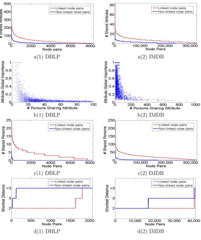
Figure 3.2: Verification of link recommendation criteria in datasets.

pairs as that of linked pairs in both data sets. As shown in Figure 3.2a, compared to the non-linked pairs, the linked pairs are more likely to share more attributes. (2) We analyze the correlation between the global importance of an attribute and the number of people sharing

(35)

the attribute. The global importance of the attribute measures the percentage of existing links among all the possible person pairs with this attribute. The larger the global weight is, the more predictive the attribute is for link recommendation. As shown in Figure 3.2b, we find that the attributes of lower frequency are likely to have higher global weights. (3) If we randomly draw a person from the linked persons, it is obvious that the selected person is more likely to have the frequent attribute in common with these linked persons. (4) We sample equal number of non-linked pairs and linked pairs. As shown in Figure 3.2c, compared to the non-linked pairs, the linked pairs are more likely to share more neighbors. (5) We construct a new graph by removing 25% linked node pairs from the original graph. We test the distances between the removed 25% node pairs in the new graph. We sample the same number of non-linked pairs as the removed linked node pairs in the original graph. As shown in Figure 3.2d, compared to the non-linked pairs in the original graph, these 25% node pairs are much closer to each other. (6) The node degree determines number of persons a particular person is linked to. A popular person is more likely to be highly linked.

3.4.3 Accuracy Metrics and Baseline

Accuracy Metrics. We remove some of the edges in the graph and recommend the links based on the pruned graph. Four-fold cross validation is used on both of the data sets in the experiment: randomly divide the set of links in the social graph into four partitions, use one partition for testing, and retain the links in other partitions. We randomly sample 100 people and recommend the top-k links for each person. We use precision, recall and mean reciprocal rank (MRR) for reporting accuracy. P@k = _|_S1_|P

p∈SPk(p) where S is the set of

sampled person nodes, Pk(p) = Nk_k(p) and Nk(p) is the number of the truly linked persons

in the top-k list of person p. recall = _|_S1_|P

p∈Srecall(p) where recall(p) =

|Fp∩Rp|

|Fp| (recall is

measured on the top-50 results). Fp is the truly linked person set of person pand Rp is the

set of recommended linked persons of person p. MRR = _|_S1_|P

p∈S

1

rankp where rankp is the

(36)

Baseline methods. To demonstrate the effectiveness of our method, we compare our method with the other methods based on the attribute and structure.

• Random: Random selection.

• SimAttr: Cosine similarity based on the attribute space.

• WeightedSimAttr: Cosine similarity based on the attribute space using global impor-tance as the attribute weight.

• ShortestDistance: The length of the shortest path.

• CommonNeighbors: score(x, y) = |Γ(x)∩Γ(y)|. Γ(x) is the set of neighbors of x in graph G.

• Jaccard: score(x, y) =|Γ(x)∩Γ(y)|/|Γ(x)∪Γ(y)|. • Adamic/Adar: score(x, y) =P

z∈Γ(x)∩Γ(y) 1 log|Γ(z)|.

• PrefAttach: score(x, y) = |Γ(x)| · |Γ(y)|. • Katz: score(x, y) =P

l=1..∞β

l_{· |path}<l>

x,y |, where β is the damping factor and path<l>x,y

is the set of all length-l paths fromxtoy. We consider the paths with length no more than 3.

To compare our method with the supervised learning methods, we use Support Vector Machine (SVM) on a combination of attribute and structure features. Specifically, we use the promising features, including SimAttr, WeightedSimAttr, CommonNeighbors, Jaccard, Adamic/Adar and Katz, for the training. Here we use the LIBSVM toolkit1_{. Both linear}

kernel and Radial Basis Function (RBF) kernel are tested. We use SVM Linear to denote the SVM method using linear kernel and SVM RBF to denote the SVM method using RBF kernel in Tables 3.3 and 3.4.

(37)

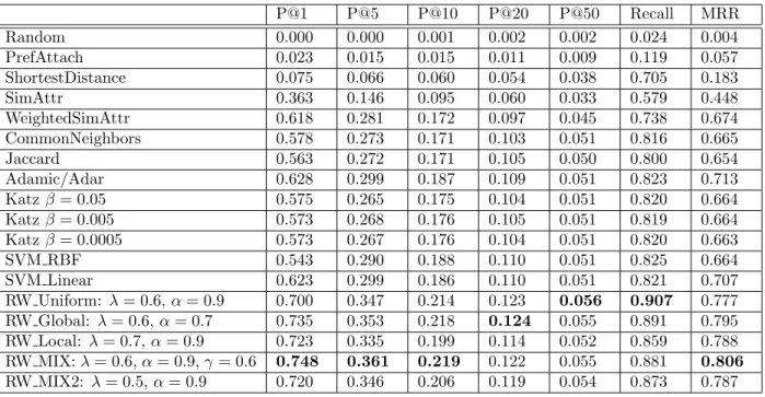
Table 3.3: Comparison of the methods in DBLP dataset. P@1 P@5 P@10 P@20 P@50 Recall MRR Random 0.000 0.000 0.001 0.002 0.002 0.024 0.004 PrefAttach 0.023 0.015 0.015 0.011 0.009 0.119 0.057 ShortestDistance 0.075 0.066 0.060 0.054 0.038 0.705 0.183 SimAttr 0.363 0.146 0.095 0.060 0.033 0.579 0.448 WeightedSimAttr 0.618 0.281 0.172 0.097 0.045 0.738 0.674 CommonNeighbors 0.578 0.273 0.171 0.103 0.051 0.816 0.665 Jaccard 0.563 0.272 0.171 0.105 0.050 0.800 0.654 Adamic/Adar 0.628 0.299 0.187 0.109 0.051 0.823 0.713 Katzβ= 0.05 0.575 0.265 0.175 0.104 0.051 0.820 0.664 Katzβ= 0.005 0.573 0.268 0.176 0.105 0.051 0.819 0.664 Katzβ= 0.0005 0.573 0.267 0.176 0.104 0.051 0.820 0.663 SVM RBF 0.543 0.290 0.188 0.110 0.051 0.825 0.664 SVM Linear 0.623 0.299 0.186 0.110 0.051 0.821 0.707 RW Uniform: λ= 0.6,α= 0.9 0.700 0.347 0.214 0.123 0.056 0.907 0.777 RW Global: λ= 0.6,α= 0.7 0.735 0.353 0.218 0.124 0.055 0.891 0.795 RW Local: λ= 0.7,α= 0.9 0.723 0.335 0.199 0.114 0.052 0.859 0.788 RW MIX:λ= 0.6,α= 0.9,γ= 0.6 0.748 0.361 0.219 0.122 0.055 0.881 0.806 RW MIX2: λ= 0.5,α= 0.9 0.720 0.346 0.206 0.119 0.054 0.873 0.787

We use RW Uniform to denote our method using uniform weighting scheme, RW Global to denote our method using global edge weighting, RW Local to denote our method using local edge weighting, RW MIX to denote our method using mixed weighting of global and local importance by linear interpolation, and RW MIX2 to denote our method using mixed weighting by multiplication of global and local attribute importance.

3.4.4 Methods Comparison

Here we compare accuracy of link recommendation using different methods on the DBLP and IMDB data sets. The results are listed in Tables 3.3 and 3.4. Random method performs the worst as expected. Since there are so many person nodes in the graph, it is almost impossible to recommend the correct links by random selection. PrefAttach and ShortestDistance perform poorly in both data sets.

Structure-based measures other than ShortestDistance perform well for both data sets. This indicates that the graph structure plays a crucial role in link recommendation. Com-pared with DBLP, precision and MRR in IMDB are much higher, but recall is lower. The

(38)

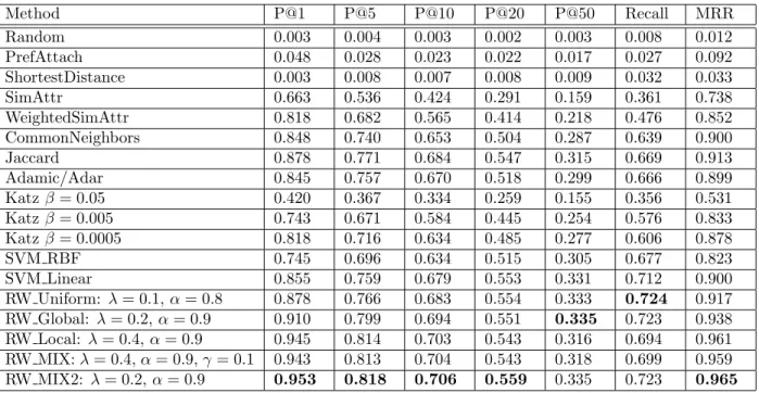
Table 3.4: Comparison of the methods in IMDB dataset. Method P@1 P@5 P@10 P@20 P@50 Recall MRR Random 0.003 0.004 0.003 0.002 0.003 0.008 0.012 PrefAttach 0.048 0.028 0.023 0.022 0.017 0.027 0.092 ShortestDistance 0.003 0.008 0.007 0.008 0.009 0.032 0.033 SimAttr 0.663 0.536 0.424 0.291 0.159 0.361 0.738 WeightedSimAttr 0.818 0.682 0.565 0.414 0.218 0.476 0.852 CommonNeighbors 0.848 0.740 0.653 0.504 0.287 0.639 0.900 Jaccard 0.878 0.771 0.684 0.547 0.315 0.669 0.913 Adamic/Adar 0.845 0.757 0.670 0.518 0.299 0.666 0.899 Katzβ= 0.05 0.420 0.367 0.334 0.259 0.155 0.356 0.531 Katzβ= 0.005 0.743 0.671 0.584 0.445 0.254 0.576 0.833 Katzβ= 0.0005 0.818 0.716 0.634 0.485 0.277 0.606 0.878 SVM RBF 0.745 0.696 0.634 0.515 0.305 0.677 0.823 SVM Linear 0.855 0.759 0.679 0.553 0.331 0.712 0.900 RW Uniform: λ= 0.1,α= 0.8 0.878 0.766 0.683 0.554 0.333 0.724 0.917 RW Global: λ= 0.2,α= 0.9 0.910 0.799 0.694 0.551 0.335 0.723 0.938 RW Local: λ= 0.4,α= 0.9 0.945 0.814 0.703 0.543 0.316 0.694 0.961 RW MIX:λ= 0.4,α= 0.9,γ= 0.1 0.943 0.813 0.704 0.543 0.318 0.699 0.959 RW MIX2: λ= 0.2,α= 0.9 0.953 0.818 0.706 0.559 0.335 0.723 0.965

reason is that on average there are much more links per person in IMDB (96.67) than in DBLP (6.63). The more the links, the more likely we can get correct link recommendations in the top results. Furthermore, dense graph structure makes structure-based measures more expressive.

Attribute-based measures (especially WeightedSimAttr) perform fairly well in both DBLP and IMDB. Accuracy achieved by WeightedSimAttr is comparable to that achieved by structure-based measures. It indicates that attribute information complements to the struc-ture feastruc-tures for link recommendation in these two data sets. WeightedSimAttr uses the global importance as the attribute weight, whereas SimAttr weighs all the attributes equally. The effectiveness of global importance score helps WeightedSimAttr to be more accurate than SimAttr.

Supervised learning methods SVM RBF and SVM Linear perform well, but cannot beat the best baseline measure in precision at top in both of the data sets. It shows that directly combining attribute and structure features using supervised learning technique may not lead to good results. Although SVM makes use of both attribute and structure properties,

(39)

it does not take into account the semantics behind the link recommendation criteria when computing the model.

Compared with the baseline methods, our methods perform significantly better in both DBLP and IMDB. In DBLP, RW MIX has the best precision (74.75% precision at 1, 36.05% precision at 5 and 21.87% precision at 10) and the best MRR (80.58%), while RW Uniform has the best recall (90.68%). In IMDB, RW MIX2 has the best precision (95.25% precision at 1, 81.80% precision at 5, 70.58% precision at 10) and the best MRR (96.48%), while RW Uniform has the best recall (72.43%). Global and local weighting methods reinforce the link recommendation criteria. Hence, RW Global, RW Local, RW MIX and RW MIX2 can beat RW Uniform in terms of precision at top and MRR. In DBLP, RW Global performs better than RW Local, because the global attributes (keywords) play an important role in link recommendation compared to very specific attributes shared with coauthors. In IMDB, RW Local performs better than RW Global, which suggests that the movie locations of the partners has a significant influence on actors. Also, in DBLP, RW MIX can beat both RW Global and RW Local, whereas in IMDB RW MIX2 can outperform RW Global and RW Local. Note that RW MIX may not always provide accuracy between that of RW Global and RW Local because some people have high local influence while some others have high global influence.

3.4.5 Parameter Setting

In our link recommendation framework, there are two parameters λ and α. We discuss how to set both parameters and how the parameter settings affect the link recommendation results.

Parameter setting. Different data sets may lead to different optimal λ and α. We obtain the best values of these parameters by performing a grid search over ranges of val-ues for these parameters and measuring accuracy on the validation set for each of these configuration settings.

(40)

Table 3.5: Recommended Persons in DBLP dataset.

Rakesh Agrawal Ricardo A. Baeza-Yates Jon M. Kleinberg Ravi Kumar Gerhard Weikum

Roberto J. Bayardo Jr. Nivio Ziviani Christos Faloutsos Andrew Tomkins Fabian M. Suchanek Ramakrishnan Srikant Carlos Castillo Jure Leskovec D. Sivakumar Gjergji Kasneci

Jerry Kiernan Vassilis Plachouras Prabhakar Raghavan Andrei Z. Broder Klaus Berberich Christos Faloutsos Alvaro R. Pereira Jr.´ Andrew Tomkins Sridhar Rajagopalan Srikanta J. Bedathur

Yirong Xu Massimiliano Ciaramita Ravi Kumar Ziv Bar-Yossef Michalis Vazirgiannis Daniel Gruhl Aristides Gionis Cynthia Dwork Prabhakar Raghavan Stefano Ceri Gerhard Weikum Barbara Poblete Lars Backstrom Jasmine Novak Timos K. Sellis

Timos K. Sellis Gleb Skobeltsyn Ronald Fagin Jon M. Kleinberg Jennifer Widom Serge Abiteboul Ravi Kumar Sridhar Rajagopalan Christopher Olston Hector Garcia-Molina Sridhar Rajagopalan Massimo Santini Deepayan Chakrabarti Anirban Dasgupta Fran¸cois Bry Rafael Gonz´alez-Cabero Sebastiano Vigna Uriel Feige Daniel Gruhl Frank Leymann

Asunción Gómez-Pérez Qiang Yang D. Sivakumar Uriel Feige Wolfgang Nejdl *Names inItalicsfont represent true positives.

Effect of λsetting. λcontrols the tradeoff between attribute and structural properties. Higher value ofλimplies that the algorithm gives more importance to the attribute features than structure features. We find the optimal λ is 0.6 in DBLP and 0.2 in IMDB, and the combination of attribute and structural features is much better than using attribute or structure properties individually.

Effect of α setting. α is the restart probability of random walks. Random walk with restart is quite popular in applications like personalized search and query suggestion. In our link recommendation setting, large α provides more accurate link recommendation, unlike lowα in traditional applications. In personalized search, random walks are used to discover relevant entities spread out in the entire graph, so a small α is favorable in those cases. However, in link recommendation task, we are more focused on the local neighborhood information, so a largeα is more reasonable. We find that α = 0.9 provides the best result. Besides high accuracy, largeα makes the algorithm converge faster.

3.4.6 Case Study

We select several well known researchers and show the recommended persons in Table 3.5 as well as top-ranked keywords for each person in Table 3.6. Since we partition the links into four partitions, the recommended persons in Table 3.5 are selected from top-3 results

(41)

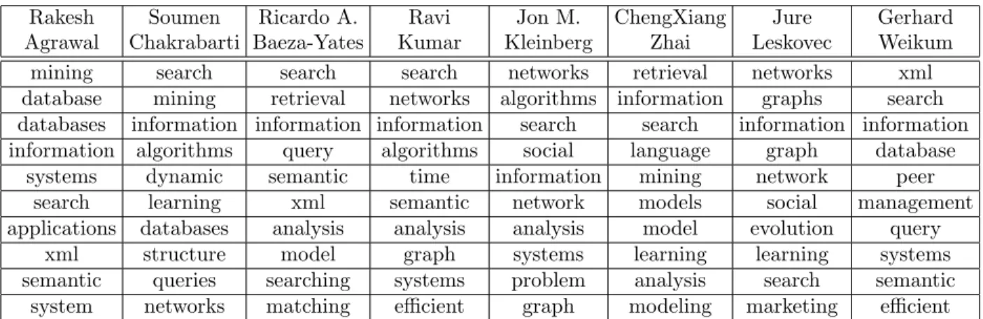
Table 3.6: Attribute Ranking in DBLP dataset.

Rakesh Soumen Ricardo A. Ravi Jon M. ChengXiang Jure Gerhard Agrawal Chakrabarti Baeza-Yates Kumar Kleinberg Zhai Leskovec Weikum

mining search search search networks retrieval networks xml database mining retrieval networks algorithms information graphs search databases information information information search search information information information algorithms query algorithms social language graph database

systems dynamic semantic time information mining network peer search learning xml semantic network models social management applications databases analysis analysis analysis model evolution query

xml structure model graph systems learning learning systems semantic queries searching systems problem analysis search semantic

system networks matching efficient graph modeling marketing efficient in each partition obtained by applying our framework using global weighting strategy. The top-ranked keywords in Table 3.6 are selected by applying our framework using uniform weighting on the complete coauthorship graph without partitioning.

3.5 Conclusions and Future Work

We propose a framework for link recommendation based on attribute and structural prop-erties in a social network. We first enumerate the desired criteria for link recommendation. To calculate the link relevance that satisfies those criteria, we augment the social graph with attributes as additional nodes and use a random walk algorithm on the augmented graph. Both global and local attribute information can be leveraged into the framework by influ-encing edge weights. Besides link recommendation, our framework can be easily adapted to provide attribute ranking as well.

Our framework can be further improved in several aspects. First, attributes may be correlated with each other. The framework should automatically identify such semantic cor-relations and handle it properly for link recommendation. Second, the algorithm currently adds a new attribute node for every value of categorical attributes. Handling numeric at-tributes would require tuning to appropriate level of discretization. We also plan to test the effectiveness of our method on friendship networks like Facebook.

(42)

Chapter 4 Latent Geographical Topic Analysis

4.1 Introduction

With the popularity of low-cost GPS chips and smart phones, geographical records have become prevalent on the Web. A geographical record is usually denoted by a two dimensional vector, latitude and longitude, representing a unique location on the Earth. There are several popular ways to obtain geographical records on the Web:

1. Advanced cameras with GPS receivers could record GPS locations when the photos were taken. When users upload these photos on the Web, we can get the geographical records from the digital photo files.

2. Some applications including Google Earth and Flickr provide interfaces for users to specify a location on the world map. Such a location can be treated as a geographical record in a reasonable resolution.

3. People can record their locations by GPS functions in their smart phones. Popular so-cial networking websites, including Facebook, Twitter, Foursquare and Dopplr, provide services for their users to publish such geographical information.

In the above three scenarios, GPS records are provided together with different docu-ments including tags, user posts, etc. We name those docudocu-ments with GPS records as GPS-associated documents. The amount of GPS-associated documents is increasing dra-matically. For example, Flickr hosts more than 100 million photos associated with tags

(43)

and GPS locations. The large amount of GPS-associated documents makes it possible to analyze the geographical characteristics of different subjects. For example, by analyzing the geographical distribution of food and festivals, we can compare the cultural differences around the world. We can also explore the hot topics regarding the candidates in presidential election in different places. Moreover, we can compare the popularity of specific products in different regions and help make the marketing strategy. The geographical characteristics of these topics call for effective approaches to study the GPS-associated documents on the Web.

In recent years, some studies have been conducted on GPS-associated documents in-cluding organizing geo-tagged photos [22] and searching large geographical datasets [49]. However, none of them addressed the following two needs in analyzing GPS-associated doc-uments.

• Discovering different topics of interests those are coherent in geographical regions. Ad-ministrative divisions such as countries and states can be used as regions to discover topics. However, we are more interested in different region segmentations correspond-ing to different topics. For example, a city can be grouped into different sub-regions in terms of architecture or entertainment characteristics; a country might be separated into regions according to landscapes like desert, beach and mountain. Unfortunately, existing studies either overlook the differences across geographical regions or employ country/state as the fixed configuration.

• Comparing several topics across different geographical locations. It is often more inter-esting to compare several topics than to analyze a single topic. For example, people would like to know which products are more popular in different regions, and sociolo-gists may want to know the cultural differences across different areas. With the help of GPS-associated documents, we can map topics of interests into their geographical distributions. None of the previous work addressed this problem and we aim to develop

(44)

an effective method to compute such comparison.

We propose three different models for geographical topic discovery and comparison. First, we introduce a location-driven model, where we cluster GPS-associated documents based on their locations and make each document cluster as one topic. The location-driven model works if there exist apparent location clusters. Second, we introduce a text-driven model, which discovers topics based on topic modeling with regularization by spatial information. The text-driven model can discover geographical topics if the regularizer is carefully selected. However, it cannot get the topic distribution in different locations for topic comparison, since locations are only used for regularization instead of being incorporated into the generative process. Third, considering the facts that a good geographical configuration benefits the estimation of topics, and that a good topic model helps identify the meaningful geographical segmentation, we build a unified model for both topic discovery and comparison. We propose a novel location-text joint model called LGTA (Latent Geographical Topic Analysis), which combines geographical clustering and topic modeling into one framework. Not only can we discover the geographical topics of high quality, but also can estimate the topic distribution in different geographical locations for topic comparison.

4.2 Problem Formulation

In this section, we define the problem of geographical topic discovery and comparison. The notations that we used are listed in Table 4.1.

Definition 1. AGPS-associated documentis a text document associated with a GPS

location. Formally, document d contains a set of words wd, where the words are from

vocabulary set V. ld= (xd, yd) is the location of document d where xd and yd are longitude

and latitude respectively. One example of a GPS-associated document can be a set of tags for a geo-tagged photo in Flickr, where the location is the GPS location where the photo was

(45)

Table 4.1: Notations used in problem formulation. Symbol Description

V Vocabulary (word set), w is a word in V D Document collection

d A document d that consists of words and GPS location

wd The text of documentd

ld The GPS location of document d

Z The topic set, z is a topic in Z

θ The word distribution set forZ, i.e.,{θz}z∈Z

taken. Another example can be a tweet in Twitter, where the location is the GPS location from the smart phone.

Definition 2. Ageographical topicis a spatially coherent meaningful theme. In other

words, the words that are often close in space are clustered in a topic. We give two geo-graphical topic examples as follows.

Example 1. Given a collection of geo-tagged photos related to festival with tags and locations in Flickr, the desired geographical topics are the festivals in different areas, such as Cherry Blossom Festival in Washington DC andSouth by Southwest Festival in Austin, etc.

Example 2. Given a collection of geo-tagged photos related to landscapewith tags and locations in Flickr, the desired geographical topics are landscape categories that are spatially coherent, such as coast, desert, mountain, etc.

We study the problem of geographical topic discovery and comparison. Given a collection of GPS-associated documents, we would like to discover the geographical topics. We would also like to compare the topics in different geographical locations. Here we give an example of geographical topic discovery and comparison.

Example 3. Given a collection of geo-tagged photos related to foodwith tags and loca-tions in Flickr, we would like to discover the geographical topics, i.e., what people eat in

Exploring link, text and spatial-temporal data in social media

Abstract

Acknowledgments

Table of Contents

List of Tables

List of Figures

Chapter 1

Introduction

Chapter 2

Related Work

2.1

Link Mining in Social Media

2.2

Text Mining in Social Media

2.3

Spatial-temporal Mining in Social Media

Chapter 3

Link Recommendation

3.1

Introduction

3.2

Problem Formulation

3.3

Proposed Solution

3.3.1

Graph Construction

3.3.2

Algorithm Design

3.3.3

Edge Weighting

3.3.4

Attribute Ranking

3.3.5

Complexity and Efficiency

3.4

Experiment

3.4.1

Datasets

3.4.2

Link Recommendation Criteria

3.4.3

Accuracy Metrics and Baseline

3.4.4

Methods Comparison

3.4.5

Parameter Setting

3.4.6

Case Study

3.5

Conclusions and Future Work

Chapter 4

Latent Geographical Topic Analysis

4.1

Introduction

4.2

Problem Formulation