Generalised linear mixed models: likelihood and Bayesian computations with applications in epidemiology

Zurich Open Repository and Archive University of Zurich Main Library Strickhofstrasse 39 CH-8057 Zurich www.zora.uzh.ch Year: 2015

Generalised linear mixed models: likelihood and Bayesian computations with applications in epidemiology

Sauter, Rafael

Abstract: Wiederholtes Messen desselben Patienten impliziert, dass die erhobenen Beobachtungen nicht unabhängig sind, da diese von denselben patientenspezifischen Eigenschaften beeinflusst werden. Ein generalisiertes lineares gemischtes Modell (GLMM) berücksichtigt diese Abhängigkeiten, indem patien-tenspezifische Modellparameter eingeführt werden, die als zufällige Effekte bezeichnet werden. Die Struk-tur der Abhängigkeiten in den Daten kann Formen annehmen, die verschieden sind von der, welche durch wiederholtes beobachten derselben Patienten auftritt. Es kann eine zeitliche, räumliche oder zeit-räumliche Abhängigkeit, im zugrunde liegenden Prozess, vorhanden sein. Auch ein Netzwerk aus verschiedenen Einheiten, die verbunden sind und wiederholt beobachtet werden, kann den Einschluss von zufälligen Effekten in einem GLMM motivieren. Ein GLMM schützt, bei gegebener Struktur der zufälligen Effekte, den bedingten Erwartungswert der interessierenden Parameter, die als fixe Effekte bezeichnet werden. Die Likelihood Inferenz bestimmt die bedingten Schätzwerte durch numerische Inte-gration uber die zufälligen Effekte, da dieses Problem generell nicht analytisch lösbar ist. Die numerische Integration kann rechnerisch schwer lösbar sein, je nach Komplexität der Struktur der zufälligen Effekte und der verfügbaren Daten. Ein Bayesianischer Inferenz Ansatz bildet die Struktur der zufälligen Effekt, unter Einschluss von Priori-Verteilungen für diese Parameter, ab. Der Einschluss von Priori-Verteilungen ist flexibel und kann die unterschiedliche, verfügbare Information auf verschiedenen Ebenen des Modells abbilden. Bayesianische Inferenz wird üblicherweise mit einer Markov-Chain-Monte-Carlo (MCMC) Sim-ulation durchgefuhrt, die eine grosse Rechenleistung verlangt. Falls der Struktur der zufälligen Effekte ausschliesslich Gaussche Priori-Verteilungen zugewiesen werden, nur eine zusätzliche Ebene von Hyperpa-rametern und eine beschränkte Ordnung der Abhängigkeiten zwischen den Einheiten angenommen wird – so dass ein Gaussches Markov Zufallsfeld resultiert – kann die Methode der integrated nested Laplace approximations (INLA) als Alternative zu MCMC verwendet werden. INLA verlangt weniger Rechenleis-tung, was insbesondere fur komplexe Modelle ein Vorteil ist. Diese Dissertation untersucht beide Inferenz Methoden fur GLMMs, diskutiert damit verbundene rechentechnische Aspekte und erläutert diese an-hand mehrerer epidemiologischen Anwendungen. Als Erstes wird die Likelihood Inferenz fur ein linear gemischtes Modell, ba- sierend auf longitudinale Daten aus der Schweizerischen HIV Kohortenstudie durchgeführt. Das Modell untersucht, ob vorherig beobachtete Lymphozyt-Subtypen relevante Prädik-toren für den Krankheitsverlauf von unbehandelten und behandelten HIV infizierte Patienten sind. Im darauf folgenden Teil wird diskutiert wie die spezielle Situation, bei welcher patientenspezifische longitu-dinale Profile keine Variation in der Ausgangsgrosse haben, die Likelihood und Bayesianische Inferenz mit

die fixen Effekte in einem GLMM angenommen. In manchen Situationen kann diese Annahme zu unre-alistischen Parameter Schätzungen führen. Adaptives gewichten der Priori-Verteilungen, basierend auf den beobachteten Daten und unter Einschluss von Korrelationen, kann dazu dienen dieses Problem zu beheben. Repeatedly observing the same patient implies that these samples will not be independent, as they are affected by the same common patient-specific characteristics. A generalized linear mixed model (GLMM) takes this dependency structure into account by introducing patient- specific model parameters which are called random effects. The dependency structure in the collected data could have various forms, though other than the one which arises from repeatedly observing patients in a study popula-tion. A temporal, spatial or even spatio-temporal pattern may be present in the underlying sampling process. Or a network of different clusters which are connected and repeatedly observed may motivate the inclusion of random effects in a GLMM. Given the random effect structure, a GLMM investigates the conditional expectation for the parameters of interest, which are called fixed effects. In likelihood inference, the conditional estimates are determined by numerically integrating over the random effects, as in general this problem is not analytically solvable. The numerical integration may be computationally difficult to solve, depending on the complexity of the random effect structure and the data at hand. A Bayesian inference approach maps the random effect structure by including prior distributions for these parameters. The inclusion of prior distributions is flexible and may reflect different stages of informa-tion at different levels of the model. Bayesian inference is commonly carried out using computainforma-tionally intensive Markov chain Monte Carlo (MCMC) sampling. If exclusively Gaussian priors are assigned to the random effect structure, with only one additional level of hyperparameters and a limited order of dependencies between clusters – such that a Gaussian Markov random field results – one can apply integrated nested Laplace approximations (INLA). INLA is an alternative to MCMC and requires less computational effort, which especially for complex models is an huge advantage. This thesis investigates both inference approaches for GLMMs, discusses related computational issues and illustrates these with several epidemiological applications. First, likelihood inference is carried out for a model based on longi-tudinal data from the Swiss HIV cohort study. This model investigates if past lymphocyte subtypes are relevant predictors for the disease progression among untreated and treated HIV infected patients. In the second part we discuss how the special situation, in which patient-specific longitudinal profiles show no variation in the response, influences the likelihood and Bayesian inference with INLA. We show that, with an increasing proportion of patients who have no variation in the response, numerical issues arise in the Maximum likelihood (ML) estimation of a binary response GLMM. Furthermore, we show that in this case INLA produces estimates that are inconsistent with ML or MCMC inference. In the third part we discuss how the particular dependency structure of a network meta-analysis is implemented with INLA, taking into account trial specific het- erogeneity and possible network inconsistencies. The last part of the thesis examines the use of informative priors which use adaptive weights that are based on the observed data. Usually the prior distributions for the fixed effects in a GLMM are assumed to be uninformative and uncorrelated. In some situations this assumption may lead to unrealistic parameter estimates. An adaptively weighted informative prior distribution may help to resolve this problem.

Posted at the Zurich Open Repository and Archive, University of Zurich ZORA URL: https://doi.org/10.5167/uzh-152199

Dissertation Published Version Originally published at:

Sauter, Rafael. Generalised linear mixed models: likelihood and Bayesian computations with applications in epidemiology. 2015, University of Zurich, Faculty of Science.

Generalised Linear Mixed Models:

Likelihood and Bayesian Computations

with Applications in Epidemiology

Dissertation

zur

Erlangung der naturwissenschaftlichen Doktorw ¨urde

(Dr. sc. nat.)

vorgelegt der

Mathematisch-naturwissenschaftlichen Fakult¨at

der

Universit¨at Z ¨urich

von

Rafael Sauter

von

Sulgen TG

Promotionskomitee

Prof. Dr. Leonhard Held (Vorsitz)

Prof. Dr. Christel Faes

Prof. Dr. Reinhard Furrer

Prof. Dr. Huldrych G ¨unthard

Preface

The last three and a half years remind me of a journey, which had an entirely unknown destination at its start. The good thing was, even though I had to walk on my own, I rarely walked alone. I would like to thank several people who supported and accompanied me. First I would like to thank Leonhard Held who made it possible for me to venture this journey and prevented it from becoming an odyssey. I am grateful for his enduring support, his patience and his close mentoring during all these years.

I would also like to thank the members of my dissertation committee, especially Christel Faes for writing the report. Further I would like to thank the research council of the Swiss HIV cohort study, which provided financial support for the corresponding project and especially to Huldrych G ¨unthard, Bruno Ledergerber and Ruizhu Huang who participated in this project and were always taking part in valuable discussions of the intermediate results.

I would also like to thank Daniel Saban´es Bov´e and Sebastian Meyer for sharing the office and the everyday life with me. Then I want to specially thank Andrea Riebler who essentially taught me everything I know about INLA and always readily provided support whenever I came to a dead end.

My thanks go also to all my former and present colleagues and members of the Biostatis-tics Department at this institute, which are without any particular order: Michaela Paul, Julia Braun, Sarah Haile, Andrea Riebler, Daniel Saban´es Bov´e, Andrea Krause, Sebastian Meyer, Wei Wei, Lorenzo Tanadini, Stefanie Muff, Burkhardt Seifert, Małgorzata Roos, Alois Tschopp, Torsten Hothorn, Heidi Seibold, Manuela Ott, Isaac Gravestok, Rachel Heyard, Eva Furrer, Sinikka Kohler, Evelyn Bielser, Niels Hagenbuch and Beate Sick. This list is certainly non-exhaustive and could be extended by many others as there are numerous other enrich-ing people at the EBPI of the University of Zurich who contributed to make my time here enjoyable.

Finally I would like to thank again Małgorzata Roos, Andrea Riebler, Julia Braun and Sebas-tian Meyer for reading and correcting the introduction chapter of this thesis.

Zusammenfassung

Wiederholtes messen desselben Patienten impliziert, dass die erhobenen Beobachtungen nicht unabh¨angig sind, da diese von denselben patientenspezifischen Eigenschaften beeinflusst wer-den. Ein generalisiertes lineares gemischtes Modell (GLMM) ber ¨ucksichtigt diese Abh¨angig-keiten, indem patientenspezifische Modellparameter eingef ¨uhrt werden, die als zuf¨allige Ef-fekte bezeichnet werden. Die Struktur der Abh¨angigkeiten in den Daten kann Formen anneh-men, die verschieden sind von der, welche durch wiederholtes beobachten derselben Patien-ten auftritt. Es kann eine zeitliche, r¨aumliche oder zeit-r¨aumliche Abh¨angigkeit, im zugrunde liegenden Prozess, vorhanden sein. Auch ein Netzwerk aus verschiedenen Einheiten, die ver-bunden sind und wiederholt beobachtet werden, kann den Einschluss von zuf¨alligen Effekten in einem GLMM motivieren.

Ein GLMM sch¨atzt, bei gegebener Struktur der zuf¨alligen Effekte, den bedingten Erwartungs-wert der interessierenden Parameter, die als fixe Effekte bezeichnet werden. Die Likelihood In-ferenz bestimmt die bedingten Sch¨atzwerte durch numerische Integration ¨uber die zuf¨alligen Effekte, da dieses Problem generell nicht analytisch l¨osbar ist. Die numerische Integration kann rechnerisch schwer l¨osbar sein, je nach Komplexit¨at der Struktur der zuf¨alligen Effekte und der verf ¨ugbaren Daten.

Ein Bayesianischer Inferenz Ansatz bildet die Struktur der zuf¨alligen Effekt, unter Einschluss von Priori-Verteilungen f ¨ur diese Parameter, ab. Der Einschluss von Priori-Verteilungen ist flexibel und kann die unterschiedliche, verf ¨ugbare Information auf verschiedenen Ebenen des Modells abbilden. Bayesianische Inferenz wird ¨ublicherweise mit einer Markov chain Monte Carlo (MCMC) Simulation durchgef ¨uhrt, die eine grosse Rechenleistung verlangt. Falls der Struktur der zuf¨alligen Effekte ausschliesslich Gaussche Priori-Verteilungen zugewiesen wer-den, nur eine zus¨atzliche Ebene von Hyperparametern und eine beschr¨ankte Ordnung der Abh¨angigkeiten zwischen den Einheiten angenommen wird – so dass ein Gaussches Markov Zufallsfeld resultiert – kann die Methode der integrated nested Laplace approximations (INLA) als Alternative zu MCMC verwendet werden. INLA verlangt weniger Rechenleistung, was insbesondere f ¨ur komplexe Modelle ein Vorteil ist.

Diese Dissertation untersucht beide Inferenz Methoden f ¨ur GLMMs, diskutiert damit ver-bundene rechen-technische Aspekte und erl¨autert diese anhand mehrerer epidemiologischen Anwendungen. Als Erstes wird die Likelihood Inferenz f ¨ur ein linear gemischtes Modell, ba-sierend auf longitudinale Daten aus der Schweizerischen HIV Kohortenstudie durchgef ¨uhrt. Das Modell untersucht, ob vorherig beobachtete Lymphozyt-Subtypen relevante Pr¨adiktoren f ¨ur den Krankheitsverlauf von unbehandelten und behandelten HIV infizierte Patienten sind. Im darauf folgenden Teil wird diskutiert wie die spezielle Situation, bei welcher patienten-spezifische longitudinale Profile keine Variation in der Ausgangsgr¨osse haben, die Likelihood und Bayesianische Inferenz mit INLA beeinflussen. Wir zeigen, dass mit einem zunehmenden Anteil an Patienten, welche keine Variation in der Ausgangsgr¨osse haben, die Maximum like-lihood (ML) Sch¨atzung der Parameter, in einem Modell mit einer bin¨aren Ausgangsgr¨osse, numerische Probleme verursacht. Weiterhin zeigen wir, dass in einem solchen Fall INLA Sch¨atzungen generiert, die weder mit ML noch mit MCMC Sch¨atzungen ¨ubereinstimmen. Im dritten Teil diskutieren wir wie die besondere Abh¨angigkeitsstruktur einer Netzwerk

Meta-Abstract

Repeatedly observing the same patient implies that these samples will not be independent, as they are affected by the same common patient-specific characteristics. A generalized linear mixed model (GLMM) takes this dependency structure into account by introducing patient-specific model parameters which are called random effects. The dependency structure in the collected data could have various forms, though other than the one which arises from repeat-edly observing patients in a study population. A temporal, spatial or even spatio-temporal pattern may be present in the underlying sampling process. Or a network of different clusters which are connected and repeatedly observed may motivate the inclusion of random effects in a GLMM.

Given the random effect structure, a GLMM investigates the conditional expectation for the parameters of interest, which are called fixed effects. In likelihood inference, the conditional estimates are determined by numerically integrating over the random effects, as in general this problem is not analytically solvable. The numerical integration may be computationally difficult to solve, depending on the complexity of the random effect structure and the data at hand.

A Bayesian inference approach maps the random effect structure by including prior distri-butions for these parameters. The inclusion of prior distridistri-butions is flexible and may reflect different stages of information at different levels of the model. Bayesian inference is commonly carried out using computationally intensive Markov chain Monte Carlo (MCMC) sampling. If exclusively Gaussian priors are assigned to the random effect structure, with only one addi-tional level of hyperparameters and a limited order of dependencies between clusters – such that a Gaussian Markov random field results – one can apply integrated nested Laplace ap-proximations (INLA). INLA is an alternative to MCMC and requires less computational effort, which especially for complex models is an huge advantage.

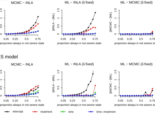
This thesis investigates both inference approaches for GLMMs, discusses related computa-tional issues and illustrates these with several epidemiological applications. First, likelihood inference is carried out for a model based on longitudinal data from the Swiss HIV cohort study. This model investigates if past lymphocyte subtypes are relevant predictors for the dis-ease progression among untreated and treated HIV infected patients. In the second part we discuss how the special situation, in which patient-specific longitudinal profiles show no vari-ation in the response, influences the likelihood and Bayesian inference with INLA. We show that, with an increasing proportion of patients who have no variation in the response, nu-merical issues arise in the Maximum likelihood (ML) estimation of a binary response GLMM. Furthermore, we show that in this case INLA produces estimates that are inconsistent with ML or MCMC inference. In the third part we discuss how the particular dependency structure of a network meta-analysis is implemented with INLA, taking into account trial specific het-erogeneity and possible network inconsistencies. The last part of the thesis examines the use of informative priors which use adaptive weights that are based on the observed data. Usually

Thesis outline

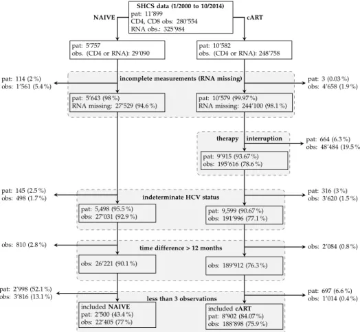
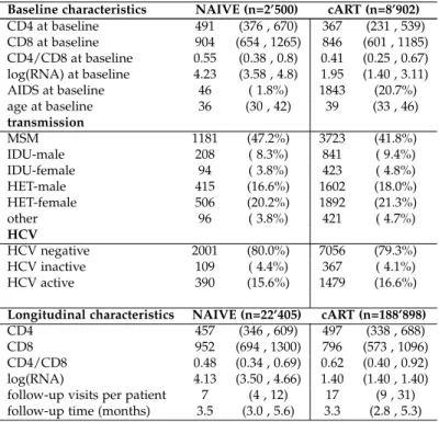
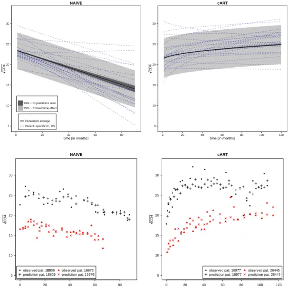
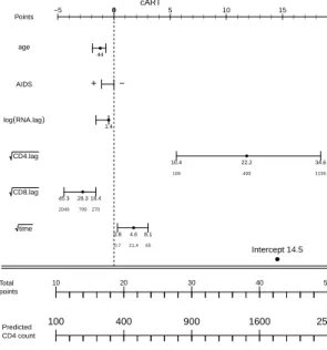
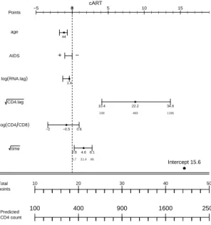
Paper I: CD8 counts and CD4/CD8 ratio independently predict CD4 response in drug naive and in patients on cART

Rafael Sauter, Ruizhu Huang, Bruno Ledergerber, Manuel Battegay, Enos Bernasconi, Matthias Cavassini, Hansjakob Furrer, Matthias Hoffmann, Mathieu Rougemont, Huldrych F. G¨unthard, Leonhard Held & the Swiss HIV cohort study.

Paper submitted toJournal of Acquired Immune Deficiency Syndromes.

Paper II: Quasi-complete Separation in Random Effects of Binary Response Mixed Models: Integrated Nested Laplace Approximations vs. MCMC

Rafael Sauter, Leonhard Held.

Paper published inJournal of Statistical Computation and Simulation.

Paper III: Network meta-analysis with integrated nested Laplace approximations

Rafael Sauter, Leonhard Held.

Paper published inBiometrical Journal.

Paper IV: Adaptive prior weighting in generalized linear models

Leonhard Held, Rafael Sauter.

Introduction

Statistical models describe deterministic and stochastic components of a data generating pro-cess by using as few parameters as nepro-cessary. In most applications model parameters map an underlying structure related to the problem. Some information about this structure may be known and thus may serve to adequately incorporate dependencies between model parame-ters. Repeatedly observing the same entities (e. g. patients), or collecting several observations under different environments (e. g. hospitals), will inherently induce possible dependencies within these entities or circumstances, which differ from the ones between entities. Taking into account and parameterizing such entity-specific dependencies is necessary, such that the observations can be considered to be conditionally independent, given the entity-specific pa-rameters. This conditional independence implies the exchangeability of the observed entities which is crucial if one considers to carry out inference for the model parameters.

The recognition and formalisation of the statistical analysis for such repeated and dependent observations dates back to more than one hundred years. Models developed during these days and for a long time thereafter were limited in their applications. Progress in the development of statistical methods but also the increasing availability of computers and more and more computing power lead to the dissemination of such models for repeated measurements. A long history of developing methods suited for particular applications, such as non-normal distributed outcomes and trials with unequally observed or unbalanced data, finally lead to the comprehensive generalized linear mixed model (GLMM) framework: a regression model class for outcomes with a distribution from the exponential family and with different types of entity-specific effects.

The generic concept of GLMMs allows to address a broad set of different applications: the dependency structure may come from independent entities, from a spatial, temporal, or com-bined spatio-temporal pattern, or may describe dependencies in any other connected graph. Longitudinal data for epidemiological studies are one of the most prominent examples, but also a meta-analysis which describes repeated observations of the same treatment comparison may make use of GLMMs. The success of GLMMs during the last years was supported by an increasing number of sophisticated, ready to use software. However, implemented algo-rithms sometimes put limitations on the distribution or the dependencies between and within different entities. Such limitations are mainly driven by the complexity of the problem, e. g. numerical integration. Computing issues arise in Bayesian as well as in likelihood based infer-ence for GLMMs. The strength of one inferinfer-ence approach may be the others weakness. Either way it is important to recognize similarities and limitations in both practices.

This chapter introduces GLMMs, including likelihood and Bayesian inference and is struc-tured in the following way: Section 1 starts with a short historical outline of the origins and the milestones in the development of the GLMM framework. Subsequently the model

as-1 Generalized linear mixed models

1.1 The origins

According to Scheff´e (1956) the idea of including different error terms for observations col-lected under different circumstances was probably first formally noted by Airy (1861, Part IV), a British astronomer. He was interested in collecting several observations of the same phe-nomena with a telescope at several nights. It was this setup which lead him to introduce in his model a special variance component for each night, reflecting the specific but varying cir-cumstances,e. g. in the atmosphere or the personal condition, encountered during each night. With this work he described the foundations of a linear mixed model, preceding the work by Fisher (1918, 1925) who laid out the same problem in a more formal way in the context of the analysis of variance (ANOVA).

The univariate repeated measures ANOVA is a precursor of the linear mixed model (LMM) which is applicable to outcomes with a normal distribution. In an ANOVA, covariates must be discrete factors, observations must be balanced, the covariance structure among repeated measures is restricted and variances assumed to be constant. The regression approach of LMMs relaxes these assumptions and allows for unbalanced and unequally spaced data, such that the number of observations per entity need not be the same and time periods between subsequent observations can vary. The inclusion of continuous covariates and more general correlation structures for the variance within an entity is also possible with a LMM. Con-tributions which were relevant in establishing LMMs also came from the interest to analyse growth curves, for which individual-specific random effects were introduced and regression coefficients were allowed to vary across individuals (Wishart, 1938; Rao, 1958). The basic prin-ciples for LMMs were established early and fundamental work has been successively added

e. g. by Harville (1976, 1977). It took some time until the application of LMMs to longitudinal data was discussed by Laird and Ware (1982).

Naturally, also models with random effects for discrete outcomes were of interest and there are several contributions,e. g. for binary data (Ashford and Sowden, 1970; Cox, 1972). In parallel Nelder and Wedderburn (1972) and McCullagh and Nelder (1989) established the generalized linear model (GLM), a framework for regression models with outcomes from any distribution that is part of the exponential family. The combination of the LMM and of GLMs lead to the extension of the model framework for repeated measures. The two methodological strains were formally embraced by the GLMM definition, described and illustrated with a broad variety of applications by Breslow and Clayton (1993). A GLMM is a regression model for an outcome from the exponential distribution family which takes dependencies for repeated observations from the same entities into account by introducing random effects. The term GLMM appears to be introduced already by Gilmouret al.(1985). Ideas for applying Bayesian inference to GLMMs evolved in parallel and were discussed by Karim and Zeger (1992). The mixed effects model approach must be distinguished from a second model framework, which is also concerned about dependencies arising from repeated measures. This other model class, known under the term marginal model, describes the population mean. This is in contrast to mixed models, also called random effects models, which investigate the entity-specific mean, conditional on the entity-entity-specific parameters. In contrast to mixed models, marginal models do not specify the full distribution but only make assumptions for the first two moments. The estimation of marginal models with generalized estimating equations

1.2 Model and data structure

A good introduction to GLMMs can be found in Fahrmeiret al.(2013, Chapter 7). The outcome of interest yij is repeatedly observed for entities i = 1, . . . ,m at occasions j = 1, . . . ,ni. The number of observation per entity ni does not have to be equal, thus a GLMM can handle unbalanced designs and the total number of observations is N = ∑m_i=1ni. The distribution of

yijcomes from the exponential family such that the GLM framework (McCullagh and Nelder, 1989) can be applied. In a GLMM the conditional expectation E(yij|xij,zij,bi)is linked to a linear predictorηij with a monotone link functionh(·)−1

h−1_{E(y

ij|xij,zij,bi)}=ηij =x>ijβ+zij>bi (1) wherexijis a vector of covariates of lengthp, including an intercept andβa vector of the same length with the parameters of interest, also called fixed effects. Usually zij is a sub-vector of xij of length q < p and bi is a vector with entity-specific parameters, or random effects, of length q. In a random intercept model qis equal to one and zij = 1. The linear predictor in Equation (1) includes one level of random effects bi. Of course one could imagine that there exist several different or nested levels of entities for which random effects could be required to correctly reflect dependencies. For the sake of keeping the notation simple we here restrict the model to one level of random effects only. Possible extensions are discussed in Section 1.3. Aggregating the data at each entity-specific level illustrates how the design matrices must be organised. All observations of one clusteriare contained in the vectoryi = (yi1, . . . ,yij, . . . ,yini)>

of lengthni. Then the linear predictor for clusteriis

ηi =Xiβ+Zibi (2) where now Xi =         x> i1 ... x> ij ... x> ini         , Zi =         z> i1 ... z> ij ... z> ini        

and Xi is a fixed effects design matrix of dimension ni×p and Zi a random effects design matrix of dimension ni×q. Aggregating the data to the next level, across all entities, results in a vector with all observations y = (y1, . . . ,yi, . . . ,ym)> of length N, such that the linear predictor is

η= Xβ+Zb.

The fixed effects design matrixXof dimensionN×pand the random effects design matrixZ

of dimensionN×qmare defined as    X> 1 ...     Z1 . . . 0  

The GLMM is complemented by the assumption that the entity-specific random effectsb1, . . . ,bm are independent and follow the same multivariate normal distribution

bi ∼N(0,D),

where D is a q×q covariance matrix. The zero expectation of bi implies that random ef-fects are symmetric deviations from the respective population mean, which is an element of

Xβ. As random effects between entities are uncorrelated, it follows that b _∼ N(0,G) and

G = diag(D1, . . . ,Dm), which is a positive definite and block-diagonal covariance matrix of dimensionqm×qm.

The following two examples give an impression on how diverse the observed data structure for repeatedly observed entities can be.

Longitudinal data

A specific disease in a study population is often observed repeatedly at several occasions for the same patients. Such longitudinal data has two sources of possible dependencies: one is from repeatedly observing the same patient, the other from possible temporal dependencies for pairs of observations from the same patienti. e. serial correlation.

Based on the notation introduced above, i would be a subscript identifying one among m

different patients that was observed at occasionj. The observations are ordered by the timestij at which they took place, which defines a sequence(ti1, . . . ,tij, . . . ,tini). Usually the temporal

ordering is considered to imply a causal relationship as described by Diggle (2002, Chapter 12). If besides a random intercept one also assumes a serial correlation between observations, then the linear predictor in Equation (2) is supplemented by an additional term such that

η_i =Xiβ+Zibi+Wi(tij), (3)

where Wi(tij) are independent realizations from a stationary Gaussian process with mean zero, variance ν2 and correlation functionρ(|tij−tik|)(see Chapter 5 in Diggle, 2002). The correlation function captures the serial correlation of the stochastic process. This functional relationship can be defined as e. g. an exponentially decaying correlation function or an au-toregressive process for discrete, equally spaced observations.

The observed outcomes for the longitudinal observations may follow a normal distribution, which requests a LMM, such as for the square root transformed CD4 lymphocyte counts in HIV-1 infected patients presented in Paper I. The outcome may also be from any other dis-tribution of the exponential family, which implies a GLMM, such as the Bernoulli distributed data for the probability of having a toenail infection presented in Paper II. The analysis of lon-gitudinal data with GLMMs is well described in Diggle (2002), by Verbeke and Molenberghs (2000) for LMMs or in Molenberghs and Verbeke (2005) for discrete outcomes.

Network meta-analysis

Evidence for a relative effect of two treatments is usually collected in a series of independent trials. Such a comparison may be extended to a set of different treatments or interventions,

assumption of possible heterogeneity in the circumstances,e. g. the different study populations which were used in the trials. The trialsi = 1, . . . ,m investigate the same relative treatment effect j among the set of different treatments 1, . . . ,T. The outcome of the GLMM may be the log odds ratio for the relative treatment comparison, which follows a normal distribution (Lumley, 2002). Alternatively, the outcome may also be the number of observed events among all study participants for each trial, which implies a binomial distributed outcome and the relative treatment effect is included as a model parameter (Lu and Ades, 2006).

1.3 Related model classes and extensions

Sometimes it is difficult to find a suitable functional relationship between an observed metric covariateuij and the outcomeyij. An extension of the linear predictor with a flexible function

f(uij)may be adequate. Possible smooth, non-linear functions forLdifferent metric covariates

uij1, . . . ,uijLcan be used as additive terms to extend the linear predictor in Equation (2) to

η_i =Xiβ+Zibi+ f1(ui1) +. . .+ fl(uil). . .+ fL(uiL). (4) In Equation (3) a similar extension was anticipated by introducing the term Wi(tij) to cap-ture serial correlation between observations. However, the function may also describe a smooth, non-parametric relationship which leads to a generalized additive mixed model (GAMM) (Ruppert et al., 2003, 2009). Generalized additive models (GAM) without entity-specific random effects but with a linear predictor which combines the component Xβ with non-parametric functional relationships are discussed by Hastie and Tibshirani (1990). The functional term fl(uil) could also describe a spatial effect for location variables uil, which leads to a geo-additive model. Fahrmeir et al.(2004) coin the term structural-additive regres-sion (STAR) for describing a model class which extends the GAMM framework. They relax the additive form of the functional relationships and allow also for non-linear interactions between two metric covariates f(u_il,u_ik)and for functions which have varying effects depend-ing on components of X. In this generic STAR setup the functional relationships can describe entity-specific random effects, a spatial, temporal or combined spatio-temporal structure but also any other form of non-linear dependency which is added to the linear predictor.

The functions f(uil)usually depend on a continuous or discrete criterion, such as the distance between two locations or two points in time. For discrete observations in timee. g. a random walk can serve as smooth function. In general one can define Markov random fields to in-troduce conditional dependencies of some order for neighbouring entities, e. g. for different regions in space (Rue and Held, 2005). Rueet al.(2009) use the term latent Gaussian model to define a subgroup of STAR models which uses a Gaussian prior for the componentsβ,b_i and on each function f(uil). The Gaussian distribution assumption for the model components is particularly attractive to use in combination with Gaussian Markov random fields (GMRF), as the sparsity of the implied structure has attractive computational properties as described by Rue and Held (2005, Chapter 2).

Here it is appropriate to draw a line to hierarchical models. Hierarchical, or multilevel mod-els are motivated from a Bayesian perspective as discussed by e. g. Gelman et al. (2014). The hierarchical approach distinguishes different levels of observational units for which

informa-sometimes called hierarchical GMRFs (Rue and Held, 2005, Chapter 4) fit into the context of hierarchical modelling. Hierarchical GMRFs use the following constitutive elements: on the first level a distribution assumption from the exponential family for observationsyij is deter-mined. The second level assumes a multivariate Gaussian prior distribution for the model componentsβ,b_i and for all functions f(uil)in the form of a GMRF. The parameters, which define the covariance structure of the GMRF, build the third level in the model hierarchy. A prior distribution is assigned again to each of these hyperparameters.

2 Likelihood inference

A compact description of likelihood inference for GLMMs can be found in Fahrmeir and Tutz (2001, Chapter 7) or Fahrmeiret al.(2013, Chapter 7). In a GLMM we assume that the outcome

yi is conditionally independent, such that we can write the conditional density for an entityi as f(yi|β,bi) = ni

∏

where here f(_·) is a density or probability mass function from the exponential family. The marginal density f(yi)can be determined by integrating over the random effects in the con-ditional density

f(yi) =

Z

f(yi|β,b)f(bi|D(δ))dbi such that the marginal likelihood for allmentities is defined as

L(β,b,δ) = m

∏

∏

where δ are unknown hyperparameters which determine the distribution of the random ef-fects covariance matrixD(δ).

2.1 Linear mixed models

For a LMM there exists an analytical solution of the integral contained in Equation (5), which results in the marginal distribution y ∼ N(Xβ,V(δ)), where V(δ) = σ2IN+ZG(δ)Z>. The residual variance is σ2 and IN is the identity matrix of dimension N. The corresponding distribution for the conditional distribution of the LMM outcome isy|b∼N(Xβ+Zb,σ2IN). For LMMs with unknown random effects covariance structure the inference problem is still challenging: one needs to find estimates forβ,b_i andδ. Maximising the LMM likelihood for βwith a fixedδgives the estimate

˜

β(δ) = (X>V(δ)−1X)−1X>V(δ)−1y

which can be derived as best linear unbiased estimator (BLUE) (Harville, 1977). Ifδis known, then the estimates for the random effects

δ, or one could use the marginal likelihood, integrating overβ

Z

L(β,b,δ)dβ (6)

to determine the estimates for the hyperparameters δ with a Fisher-scoring algorithm. The marginal likelihood in Equation (6) can be embedded into the restricted maximum likelihood (REML) approach for linear models. The REML estimation corrects the bias of the Maximum likelihood (ML) covariance parameter estimates (Diggle, 2002, Chapter 4.5). For LMMs the ML estimator based on the profile likelihood ignores the loss of degrees of freedom for estimating the fixed effects, thus is biased and so in general the REML approach should be preferred.

2.2 Generalized linear mixed models

In contrast to LMMs there is no analytical solution for the integral in Equation (5) for GLMMs. A GLMM requires a numerical integration over the q-dimensional vector bi in the marginal likelihood. There exist different approaches to solve this task. One could apply a Laplace ap-proximation (see Held and Saban´es Bov´e, 2014, Appendix C). Laplace’s method approximates the integral R f(x)dx = R exp(logf(x))dx by applying a Taylor series expansion around x?, which is the mode x? _{= argmax}

xlogf(x). This implies that the first derivative at x = x? is zero and logf(x)_≈logf(x?_{) +} (x−x?)2 2 ∂2logf(x) ∂x2 x=x? which results in an approximation of the integral with a Gaussian kernel

Z f(x)dx≈ f(x?₎Z _exp −(x−x ?₎2 2σ?2 dx

whereσ?2 is equal to the inverse, negative second derivative forxevaluated atx?.

Alternatively one can also approximate the marginal likelihood in Equation (5) with a Gauss-Hermite approximation (see Fitzmaurice et al., 2008, Chapter 4). Instead of using b it is useful to use a Cholesky decomposition of the random effects covariance D(δ), such that

bi = D(δ)1/2b?_i, and an independent standard normal distribution for b?_i ∼ N(0,I) results. For each random effectb?

ik, among qrandom effects for entityi, the one dimensional integral can be approximated by Z ni

∏

∑

∏

i,−kis a vector with all standardized random effects for entityi, except thekth one and

wr,arare the weights and locations of the Gauss-Hermite quadrature rule of degree(2R−1) (Stroud and Secrest, 1966). The quadrature points and weights can also be defined adaptively (Pinheiro and Bates, 1995), such that they depend on the cluster-specific mean and variance, which results in an improved approximation (Lesaffre and Spiessens, 2001; Rabe-Hesketh et

Stiratelliet al.(1984) proposed to use a penalized quasi-likelihood approach (PQL) for GLMMs. Breslow and Clayton (1993) motivate the PQL estimation for GLMMs with a Laplace approx-imation to the marginal likelihood. They state that the likelihood

L(β,b;δ) = f(y|b,β)f(b|D(δ)) can be rewritten as penalized log-likelihood of the form

l(β,b,δ) =l(β,b)₋ 1

2b>G(δ)−1b (7)

where l(β,b) = ∑mi=1∑nj=i1 f(yij|β,b) is the log-likelihood of the implied GLM, and the pe-nalization term₋b>_G(δ)−1_{bfollows from the normal distribution assumption for f(b). The}

PQL approach uses some starting values for β, b and δ and computes working responses which are used to solve the score functions of the penalized likelihood for β,b. In a second step the estimates forδare found by numerically solving the restricted likelihood with Fisher scoring by using the estimatesβ andb from the first step. The two steps are iteratively re-peated until the required convergence criteria are met. The score functions are the same as for the LMM but with different weights. Thus this iteratively reweighted least squares (IRLS) algorithm can also be applied to LMMs to improve estimates of δ. Estimation with PQL can yield a substantial bias, especially for binary responses with few observations per patient. Therefore there were efforts in adapting the penalization criterion to establish a bias correction by Breslow and Lin (1995) and Lin and Breslow (1996) which was even taken further by using Laplace approximations based on a Taylor series expansion of higher order by Raudenbushet al.(2000).

The second common estimation algorithm for GLMMs also involves two steps: first the es-timates for b are determined by a penalized iteratively reweigthed least squares (P-IRLS) algorithm (Bates and DebRoy, 2004) withβ, b and δ fixed at some starting values. The pe-nalized least squares criterion is optimized by iteratively updating estimates for b and then reweighting the working responses until convergence. In the second step the marginal like-lihood is approximated with a Laplace or Gauss-Hermite approximation, given the estimates

b from the first step, which is then maximized for β and δ. Both steps are repeated until convergence of the deviance₋2l(β,b,δ)is reached.

In general, ML inference for GLMMs will neglect any uncertainty coming from the estimation of the random effects b. Furthermore, the penalization term in Equation (7) is proportional to G(δ)−1 which reflects the inverse of the random effect variance. If G(δ) → ∞ then the penalization term goes to zero, such thatbwill not be treated differently than the fixed effects β. The penalization also increases for increasing deviations from E(b) = 0. The penalization term has an influence on the estimates for bi, which are shrunk more towards the overall mean Xβ with increasing entity-specific random effect variance D(δ). Also fewer numbers per entityni result in stronger shrinkage for the correspondingbi. For LMMs the EBLUP can be shown to be a weighted average between the population averaged mean response profile and the entity-specific response profile and the weight depends on the relation between the entity-specific within variance σ2Ini and the overall variance V(δ) (Fitzmaurice et al., 2004,

Chapter 8.6).

scribed as complete separation, because one covariate perfectly predicts the outcome, or as quasi-complete separation if the covariate predicts a subset of the outcome (Albert and An-derson, 1984). Firth (1993) suggested a penalized likelihood approach to solve this problem for GLMs. However, for GLMMs the complete separation problem may also be present for the entity-specific effects bi. Depending on the proportion of clusters which have no varia-tion, this cluster-specific quasi-complete separation may cause numerical instabilities in the marginal likelihood approximation.

2.3 Software

Nowadays there exist several software packages for likelihood inference in GLMMs. The following overview is restricted to software packages inR(R Core Team, 2015), although other

statistical software has similar routines implemented, likePROC NLMIXEDin SAS orxtmelogit

for logistic GLMMs in Stata. For R the most commonly used packages are nlme (Pinheiro

et al., 2015) which is for LMMs only, its extension to GLMMs with the function glmmPQL

in the package MASS (Venables and Ripley, 2002) and the package lme4 (Bates et al., 2014).

There are several differences between the packages: the estimation algorithm, the covariance structure for the random effects and whether they can include serial correlation. The software packages differ also with respect to the combination of multiple random effects they allow for, especially whether crossed random effects (i. e. each second level is observed within each first level random effect) and whether nested random effects (i. e. each second level random effect varies within each first level random effect) are possible.

Package: nlme MASS lme4

Model: LMM GLMM GLMM

Function name: lme glmmPQL glmer

Algorithm: IRLS PQL-IRLS P-IRLS

Marginal likelihood: Laplace Laplace Gauss-Hermite or Laplace

Random effects: nested only nested only nested and crossed

CovarianceD(δ): generic generic diagonal or unstructured

Table 1.: Comparison of commonRsoftware packages for likelihood inference in GLMMs.

An overview for the comparison of these criteria is given in Table 1. Serial correlation models are only available for nlme and glmmPQL. The within-correlation can be generically defined

by the user or a predefined correlation structure, such as an exponential correlation, can be used. In lme4 the random effects covariance is assumed to be unstructured or diagonal

i. e. uncorrelated, and has no possibility for serial correlation. Each package involves an IRLS algorithm with Fisher scoring based on similar numerical optimization routines. Nevertheless, the algorithms differ between packages: nlme updates the estimates for δ to increase the accuracy, glmmPQL applies the PQL algorithm and lme4 uses the P-IRLS algorithm. For the

3 Bayesian inference

Model parameters are treated as unknown random quantities in a Bayesian inference ap-proach. This is in contrast to likelihood inference where model parameters are assumed to be true, fixed quantities. The basis for Bayesian inference is Bayes’ theorem or Bayes’ rule, which states how the conditional probability of an event can be reformulated as probability of the condition, given the event. The theorem is named after Reverend Thomas Bayes, whose work on probabilities of a binomial distribution was posthumously published in 1763. Bayes’ rule for probabilities can be applied to f(_·), a density function or probability mass function. It states that the so called posterior probability distribution of the unknown parametersθ given the observed datayis

f(θ_|y) =f(y|θ)f(θ)

f(y) , (8)

where f(y) =R f(y|θ)f(θ)dθis the marginal distribution function and in the case of discrete values for θ is obtained by f(y) = ∑θ f(y|θ)f(θ). The marginal likelihood in the

denomi-nator in Equation (8) serves as normalizing constant which is independent ofθsuch that one can write

f(θ_|y)∝ f(y|θ)f(θ). (9)

The distribution of the parameters f(θ)is called prior distribution and f(y|θ)is the sampling distribution, which in likelihood inference, under the assumption ofθ being fixed quantities, is just the likelihood L(θ) = f(y|θ). Equation (9) states that the posterior distribution is proportional to the likelihood times the prior distribution. It also shows that if the prior distribution f(θ)is flat,i. e. uninformative, then the likelihood is just multiplied by a constant such that the posterior mode will coincide with the ML estimate. It also gets clear from Equation (9) that the influence of the prior relative to the likelihood decreases with increasing sample size. Adding observations will increase the product, or on the log-scale the sum, involved in the likelihood term f(y|θ) and thus increase its relative weight, compared to the prior. The posterior distribution f(θ_|y) is the fundament for inference about θ. If one is interested in a particular model parameter θk then one examines the marginal posterior distribution

f(θk|y) =

Z

f(y|θ)f(θ)dθ_−k (10)

where θ_−k are all but the kth model parameter in θ. The marginal posterior can be used to obtain interval estimates, or point estimates for θk. This can e. g. be the posterior mean

E(θk|y) =R θkf(θk|y)dθk, the posterior mode Mode(θk|y) =arg maxθk f(θk|y)or a credible

interval[tl,tu]with credible level CIψ=

Rtu

tl f(θk|y)dθk. The lower and upper bound are equal

to the quantiles tl = (1−ψ)/2 and tu = (1+ψ)/2 such that θk is within this interval with probabilityψ. An introduction to Bayesian inference is given by Held and Saban´es Bov´e (2014,

Chapter 6).

3.1 Posterior distributions for generalized linear mixed models

As mentioned in Section 1.2, the GLMM can be expressed as Bayesian hierarchical model. A Gaussian prior is assigned to the model parameters θ = (β,b)>, with b ∼ N(0,D(δ)). The distribution of the random effects is the same as in likelihood inference in Section 2. A

assigns a prior distribution to the hyperparameters of the latent Gaussian fieldθ, which are the parametersδthat define the random effects covariance matrix and which will be included as additional factor in the computation of the posterior distribution. The model parameters θ define a latent Gaussian field, for which the elements are conditionally independent, given the entity-specific stochastic dependence structure, such that a GMRF with a sparse precision matrixQ(δ)results (Rue and Held, 2005, Chapter 4). The posterior distribution for the GLMM model parameters and hyperparameters, given the datayis

f(θ,δ_|y)∝ f(δ)f(θ_|δ) I

∏

∑

as discussed by Fong et al.(2010) who review the GLMM applications presented by Breslow and Clayton (1993) in the context of Bayesian inference for hierarchical latent Gaussian models. The marginal posterior distribution for a GLMM of thekth model parameterθk is then

f(θk|y) = Z δ Z θ₋k f(θ,δ_|y)dθ₋kdδ = Z δ f(θk|δ,y)f(δ|y)dδ (11)

and for thekth component of the hyperparameters the marginal posterior distribution is

f(δk|y) =

Z

δ₋k

f(δ_|y)dδ₋k (12)

where θ_−k and δ_−k are vectors with all components in the corresponding parameter vector except thekth one.

The possibilities to apply Bayesian inference used to be limited, as the integrals in Equation (10), or respectively in (11) and (12) and the summary statistics based on these marginal pos-terior distributions were only analytically solvable for selected problems. This was e. g. the case if likelihood and posterior were conjugate, i. e. posterior and prior belong to the same distribution family. From a Bayesian point of view Equation (5) in Section 2 for LMMs is in accordance with the desirable setting of having a conjugate prior distribution, namely a normal distribution for the likelihood and for the random effects, which results in an analyt-ically solvable problem with a normal posterior distribution. The development of computers opened up the possibility of numerical integration. Coming along with the increase and avail-ability of computing power, Bayesian inference experienced a boom during the nineties of the last century (Robert and Casella, 2011), using Markov chain Monte Carlo (MCMC) sampling. In the meantime also other strategies for evaluating integrals as in Equation (10) were estab-lished, such as the integrated nested Laplace approximations (INLA) (Rue et al., 2009). Both methods, MCMC and INLA, are shortly introduced in the following two sections.

(MC) integration with computers was explored at the Los Alamos research center during the Second World War. An MC integration approximatese. g. the mean of the posterior f(θ|y), where θ is a scalar parameter. MC integration generates L independent random samples θ(1), . . . ,θ(l), . . .θ(L)from the posterior distribution and computes the mean as

E(θ|y) = Z θf(θ|y)dθ ≈ _L1 L

∑

which converges to the true value E(θ|y) for L → ∞. Similarly, one can construct estimates by using MC integration for other summary statistics based on the posterior distribution. Obtaining independent samples from the posterior distribution is difficult if there are many unknown model parametersθ. Sampling from the distribution of a high-dimensional vector θ may result in large and persistent correlations between samples. A solution to this prob-lem is to simulate a Markov chain θ(1), . . . ,θ(l). . . ,θ(L), which generates samples θ(l) that depend only on the previous sampleθ(l−1) and which converges to the posterior distribution

f(θ_|y). Given that the Markov chain converged to the posterior distribution one can again apply MC integration to obtain the summary statistics of interest. The combination of the two eponymous procedures defines MCMC sampling. The Metropolis Hastings algorithm (Metropoliset al., 1953; Hastings, 1970) describes how a Markov chain can be generated such that it converges to the posterior distribution. Starting with some values for model parameter

θk a proposal θk? is defined by drawing randomly from the proposal density f? θ?k|θk,θ−k which depends only on the current valueθ(l) of the simulated Markov chain. The parameter is updated toθ_k(l+1)=θ?_k with acceptance probability αequal to

α=min   1, f θ?_k|θ_−k,y fθ(_kl)|θ_−k,y f?_θ(l) k |θ?k,θ−k f?_θ? k|θ (l) k ,θ−k   

and otherwise θ_k(l+1) =θ_k(l). Each model parameter θk inθ can be updated, conditional on all other current model parametersθ_−k with some proposal density f?(_·)and the MH algorithm will converge to the posterior distribution if Lis large enough.

The Gibbs sampler, introduced by Geman and Geman (1984) and later discussed by Gelfand and Smith (1990), modifies the MH algorithm by setting f?_θ?

k|θ(kl),θ

(l)

−k

= f θ_k?|θ_−k,y

i. e. the proposal density is equal to the target posterior density. The Gibbs algorithm thus samples component-wise from the full conditionals of every model parameter θk and has an acceptance probability equal to one. Instead of component-wise updating every θk one can use block-updating schemes (Rue and Held, 2005, section 4.1.2), which is preferable if model parameters are highly correlated, which is discussed by Gamerman (1997) in the context of GLMMs. The hypothesis that the generated Markov chain converged to a stationary posterior distribution must be examined for every model parameter by e. g. visual inspection of the trace plots, examination of the autocorrelation function of the samples or checking different convergence diagnostics (Cowles and Carlin, 1996).

approximates the marginal posterior distribution f(θk|y,δ)for a Bayesian hierarchical model with a latent Gaussian field that follows a GMRF and which has relatively few, say less than six, hyperparameters according to Rueet al.(2009).

The first task is to approximate the joint distribution of all hyperparameters f(δ_|y), which appear in Equation (11) and from which the marginals in Equation (12) can be derived. The distribution of the hyperparameters is approximated by

f(δ_|y) = f(θ,δ|y) f(θ_|δ,y) ∝ f(y|θ,δ)f(θ_|δ)f(δ) f(θ_|δ,y) ≈ f(y|θ,δ)f(θ_|δ)f(δ) ˜ fG(θ|δ,y) θ=θ?_(δ) = f˜(δ_|y) (13) where ˜fG(θ|δ,y) is a Gaussian approximation to the full conditional of θ evaluated at the modeθ?(δ)for a givenδ. The approximation ˜f(δ_|y)corresponds to the Laplace approxima-tion to marginal posteriors discussed by Tierney and Kadane (1986). The proporapproxima-tionality in (13) is with respect to the normalizing constant f(y)in the posterior distribution f(θ,δ_|y). The approximation to the second term in Equation (11) can be done with three different methods, with different levels of accuracy. The first, simplest and least accurate approach is to use ˜fG(θ|δ,y)and derive a normal distribution to approximate each marginal distribution

˜

fG(θk|δ,y) using the mean of the Gaussian approximation and the marginal variance. As there may be errors due to shifts in location or due to skewness (Rue and Martino, 2007), a second Laplace approximation to the marginal f(θk|δ,y)by the approach of Tierney and Kadane (1986) results in a higher accuracy.

This full Laplace approximation is obtained by

f(θk|δ,y) = _ff(_(θθk,θ−k|δ,y) −k|θk,δ,y) = f(θ,δ_|y) f(δ_|y) 1 f(θ_−k|θk,δ,y) ∝ f(θ,δ,y) f(θ_−k|θk,δ,y) ≈ f(θ,δ,y) ˜ fG(θ−k|θk,δ,y) θ₋k=θ?₋k(θk,δ) = f˜(θk|δ,y) (14) where ˜fG(θ−k|θk,δ,y)is a Gaussian approximation to the full conditional f(θ−k|θk,δ,y) eval-uated at the modeθ₋?_k of the full conditional for a givenθ_−k and givenδ. The approximation

˜

fG(θ−k|θk,δ,y)requires a high computational effort as it needs to be evaluated for each en-tity in the GMRF and for each δ. Thus Rue et al. (2009) suggest two simplifications. First, they propose to use conditional densities derived from the already computed approximation

˜

fG(θ|δ,y) from Equation (13) to approximate the mode θ₋?k(θk,δ). Secondly, they restrict the influence of θ_−k on the approximation forθk, as the dependence between two entities in the GMRF is assumed to decay with increasing distance. With these two simplifications the Laplace approximation ˜f(θk|δ,y)corresponds to the Gaussian approximation multiplied by a term which is equivalent to a cubic spline for each entity-specific parameterθ_k.

The accuracy and computational costs of the third approximation, called simplified Laplace approximation, is between the simple Gaussian and the more precise full Laplace approxima-tion. The simplified Laplace approximation applies a Taylor series expansion up to the third

For INLA both terms, ˜f(δ_|y)and ˜f(θk|δ,y), are used to numerically integrate over different integration pointsδu and different weights∆u

˜

f(θk|y)≈

∑

˜

f(θk|δu,y)f˜(δu|y)∆u ₍₁₅₎

to get the approximated marginal posterior distribution ˜f(θk|y). The choice of the pointsδu and the weights∆uis discussed in more detail in Section 3.5.

INLA was demonstrated to deliver accurate approximations of the marginal posterior distri-butions coming with reduced computational costs compared to MCMC. See Rue et al.(2009) for examples or Schr¨odleet al. (2011) for applications to spatio-temporal models. Lindgrenet al.(2011) illustrate the numerical advantages of sparse matrices implied by GMRFs for large geostatistical models which are solved fast and accurately by INLA. For the applicability of INLA to GLMMs see Rueet al.(Section 5.2 2009) and Fonget al. (2010).

3.4 Choice of prior distribution

Selecting a prior distribution for f(θ)and disclose its influence on the posterior distribution is one of the most disputed elements in Bayesian inference. Gaining new knowledge about θ based on the inclusion of prior beliefs may come with the flavour of being subjective,i. e. biased and was criticised beyond the field of statistics (Popper, 1959). On the other hand, Bayes’ theorem offers a rationale on how historical data, which was observed and perhaps should not be ignored, could be taken into account and how to evaluate it in the context of new evidence. Historical data from similar previous studies may be available, which is rather common for clinical trials and could serve as prior information, also by introducing a prior weight on the historical data directly, like suggested by Ibrahim and Chen (2000).

Depending on the choice of the prior distribution, one may establish links between Bayesian inference and a ML approach. For instance, a Bayesian interpretation of the REML in LMMs is discussed by Harville (1974). One could choose a non-informative, flat prior which is proportional to a constant on the fixed effects f(β) ∝ c and as well for the hyperpameters

f(δ)∝c. The mode of the joint posterior distribution with respect toδis in this case equivalent to the ML estimate of the hyperparameters. In contrast, the mode of the the marginal posterior distribution with respect toδis equivalent to the REML estimate ofδ, which is also mentioned in Section 2.1.

Instead of assigning a prior distribution on the hyperparameters one could assume unknown and fixed values for δ. An estimate for δ could be obtained by maximizing the marginal likelihood, which results in the REML estimate for δ. Using this REML estimate of the hy-perpameters to analyse the posterior mean of β andb results in the same EBLUP estimates for β and b as in Section 2.1. This approach, without assigning a prior distribution to δ, is called empirical Bayes. Also for GLMMs the posterior modes, based on Bayesian inference with empirical Bayes, correspond to the ML estimates.

A fully Bayesian approach, in contrast to empirical Bayes, assigns a prior distribution to all parameters θ and additionally to the hyperparameters δ. The choice of a non-informative, improper prior for δ, which does not integrate to unity, does not guarantee in general that the posterior distribution will be proper. This holds also especially for Jeffreys’ prior, which is invariant to a reparametrisation. Usually one resorts to choose a weakly informative prior

tribution of b, meaning that f(σ_RI2 |b)again belongs to an inverse gamma distribution. One could of course choose the parametersα1 andα2, such that the prior is only weakly

informa-tive. The extension of this conjugate prior to the case where q > 1, e. g. a random intercept plus slope model, with aq_×qrandom effects covariance matrix, leads to an inverse Wishart distribution (Held and Saban´es Bov´e, 2014) forD(δ). Fonget al.(2010) motivate the choice of an informative prior in GLMMs for such an inverse gamma or inverse Wishart distribution. However, the inverse gamma prior on random effect variances like σ_RI2 was found by Roos

and Held (2011) to result in a large sensitivity for the parameter estimates. As an alternative, they propose to use a half-normal prior distribution on the standard deviation, which is also suggested by Gelman (2006). Gelmanet al.(2008) discusses how to assess a weakly informative default prior in the context of hierarchical models.

On the other hand, there may occur situations, such as sparse data, for which an explicit informative prior on β may be favourable (Greenland, 2006). The choice of an informative prior forδaffects the amount of shrinkage for the estimates of b_i. In Section 2 the estimates were asserted to be shrunk towards the population averaged mean response profile. As the posterior is obtained by multiplying likelihood and prior distribution, the location and the amount of shrinkage forbi can directly be influenced by choosing the moments for the prior distribution which is assigned to δ. The problem of (quasi) complete separation, mentioned in Section 2, may be put into the context of a sparse data problem (Firth, 1993). In the case of a binary covariate in a binomial GLM, where the ML estimates are not defined, complete separation arises if the off diagonal entries of the corresponding 2×2 contingency table are zero. According to Firth (1993) this can be addressed by a penalized likelihood, for which the penalization term depends on the inverse Fisher information and is related to Jeffreys’ invariant prior. For a logistic regression with a completely separating binary covariate this approach corresponds to adding 1/2 to each cell of the 2×2 table. A penalization term is in this situation related to a Bayesian approach which assigns an informative prior distribution, based on which the implied shrinkage may help to solve the problem of a non-existent ML estimate in a consistent way.

Similarly, according to Greenland (2006, 2007a,b, 2009) the use of proper, informative priors may helpe. g. in epidemiological studies with few data, to avoid possibly unrealistic assump-tions of a likelihood inference approach. For the fixed effects in a Bayesian hierarchical re-gression, the normal prior β _∼ N(0,Σβ), is usually chosen such that Σβ is diagonal with

large values for the corresponding variances. An informative prior would motivate smaller variances for some components of β and possibly also deviate form the mean zero location parameter. In Paper IV such informative priors are proposed for GLMs as well as for GLMMs, which is in line with the motivation by Greenland (2006). Furthermore, in Paper IV also the diagonal structure for Σβ is relaxed and a prior weight, based on the observed correlations

in the data, is used forβ. These adaptive prior weights are perfectly treatable with the INLA approach and were implemented by using the r-inla software. Motivating an informative

prior or using default or reference priors will not circumvent the indispensable questions about the impact of the prior and the sensitivity of the estimates with respect to alternative prior specifications. Investigating prior sensitivity becomes attractive with computationally less intensive methods such as INLA (Roos and Held, 2011; Rooset al., 2015), compared to the

3.5 Software

There also exist several software packages for Bayesian inference in GLMMs. In the follow-ing, a short overview is given for generic MCMC samplers and the r-inla package, which

implements the INLA approach discussed in Section 3.3.

MCMC

After the potential of MCMC sampling for Bayesian inference was recognized it did not last long until efforts for a common computer language which implements generic Gibbs samplers and which allows for a broad set of different applications, were initiated (Gilks et al., 1994). This resulted in the BUGS (Bayesian Inference Using Gibbs Sampling) project (Lunn et al., 2009), which defined a program language for generic MCMC samplers like Win-BUGS and Open-BUGS (Lunnet al., 2000), JAGS (Plummer, 2003). They all have a common syntax to set up Bayesian hierarchical models. These generic MCMC samplers can be used for hierarchical models with several layers of parameter levels and are not restricted to latent Gaussian fields. There are several interfaces, like the Rpackage R2jagsorcoda among others, which provide

access to the flexible Renvironment and a collection of specific functions to analyse MCMC

sampling results. Another common software package inRisMCMCglmm(Hadfield, 2010) which

is a MCMC sampler for multivariate GLMMs, uses a similar syntax as the packagenlme and

allows for correlated random effects. Yet another software package, called STAN Gelman et al. (2014); Stan Development Team (2014), uses a distinct modelling language and different methods for MCMC sampling. Most of these MCMC samplers implement a Gibbs sampler, or a general Metropolis Hastings algorithm. Nevertheless, there may be crucial differences in the implemented algorithms, for example if it comes to block updating, wheree. g. JAGS uses the algorithm proposed by Holmes and Held (2006).

INLA

The R package r-inla (Rue et al., 2014), which is available on http://www.r-inla.org, is

essentially an interface to the standalone packageINLAwhich in turn calls theGMRFLiblibrary

(Rue and Held, 2005) which is written in C and Fortran. Ther-inlapackage defines models

with a similar syntax like the establishedglmregression model framework inRand offers the

possibility to process results by the flexible facilities of theRenvironment.

Gaussian approximations to the marginal posterior (Tierney and Kadane, 1986) are obtained

in r-inlaby a Fisher scoring algorithm based on numerical optimization routines. The

ap-proximation to the joint posterior of the hyperparameters f(δ_|θ,y)involves three steps: first the mode is searched by a quasi-Newton method involving differences between gradients. The second step evaluates the curvature at the mode to get the Fisher information matrix and for which an Eigen decomposition is computed. Based on the standardized, orthogonal components the approximated posterior ˜f(δ_|y)is explored. The points δu in Equation (15) at which ˜f(δ_|y)is explored can be determined by two different strategies: the first places a grid of ’interesting’ points around the mode in each direction of the standardized variables with a certain step-length, as long as the difference in the log-densities does not exceed a stop-ping criterion. The second integration strategy, the central composite design (CCD) (Rue et al., 2009, Section 6.5), explores the posterior density with less points, thus is less accurate and