P
ANEL
U
NIT
R
OOT
T
ESTS IN THE
P
RESENCE OF A
M
ULTIFACTOR
E
RROR
S
TRUCTURE
M.
H
ASHEM
P
ESARAN
L.
V
ANESSA
S
MITH
T
AKASHI
Y
AMAGATA
CES
IFO
W
ORKING
P
APER
N
O
.
2193
C
ATEGORY
10:
E
MPIRICAL AND
T
HEORETICAL
M
ETHODS
J
ANUARY
2008
An electronic version of the paper may be downloaded
• from the SSRN website: www.SSRN.com
• from the RePEc website: www.RePEc.org
• from the CESifo website:
Twww.CESifo-group.org/wp
TCESifo Working Paper No. 2193
P
ANEL
U
NIT
R
OOT
T
ESTS IN THE
P
RESENCE OF A
M
ULTIFACTOR
E
RROR
S
TRUCTURE
Abstract
This paper extends the cross sectionally augmented panel unit root test proposed by Pesaran
(2007) to the case of a multifactor error structure. The basic idea is to exploit information
regarding the unobserved factors that are shared by other time series in addition to the
variable under consideration. Importantly, our test procedure only requires specification of the
maximum number of factors, in contrast to other panel unit root tests based on principal
components that require in addition the estimation of the number of factors as well as the
factors themselves. Small sample properties of the proposed test are investigated by Monte
Carlo experiments, which suggest that it controls well for size in almost all cases, especially
in the presence of serial correlation in the error term, contrary to alternative test statistics.
Empirical applications to Fisher’s inflation parity and real equity prices across different
markets illustrate how the proposed test works in practice.
JEL Code: C12, C15, C22, C23.
Keywords: panel unit root tests, cross section dependence, multi-factor residual structure,
Fisher inflation parity, real equity prices.
M. Hashem Pesaran
University of Cambridge
Faculty of Economics
Austin Robinson Building
Sidgwick Avenue
UK - Cambridge, CB3 9DD
[email protected]
L. Vanessa Smith
Centre for Financial Analysis and Policy
(CFAP)
Judge Business School
University of Cambridge
Trumpington Street
UK - Cambridge CB2 1AG
[email protected]
Takashi Yamagata
Department of Economics
University of York
UK - Heslington, York, YO10 5DD
[email protected]
December 2007
We would like to thank Serena Ng for sharing her codes with us for the calculation of the Bai
and Ng (2007) statistics, Joachim Westerlund for useful comments on an earlier version of the
paper, as well as participants at the conference in honour of Paul Newbold at the University of
1
Introduction
There is now a sizeable literature on testing for unit roots in panels where both cross section
(
N
) and time (
T
) dimensions are relatively large. Reviews of this literature are provided in
Banerjee (1999), Baltagi and Kao (2000), Choi (2004), and more recently in Breitung and
Pesaran (2007). The so called …rst generation panel unit root tests pioneered by Levin, Lin
and Chu (2002) and Im, Pesaran and Shin (2003) focussed on panels where the idiosyncratic
errors were cross sectionally uncorrelated. More recently, to deal with a number of applications
such as testing for purchasing power parity or output convergence, the interest has shifted to
the case where the errors are allowed to be cross sectionally correlated using a residual factor
structure.
1These second generation tests include the contributions of Moon and Perron (2004),
Bai and Ng (2004, 2007) and Pesaran (2007).
2The tests proposed by Moon and Perron (2004)
and Pesaran (2007) assume that under the null of unit roots the common factor components
have the same order of integration as the idiosyncratic components, whilst the test procedures
of Bai and Ng (2004, 2007) allow the order of integration of the factors to di¤er from that of the
idiosyncratic components, by assuming di¤erent processes generating the two. A small sample
comparison of some of these tests is provided in Gengenbach, Palm and Urbain (2006).
In the panel unit root test proposed by Pesaran (2007) cross section dependence is accounted
for by augmenting the individual ADF regressions of
y
itwith cross section averages of the
dependent variable (current and lagged values,
y
t,
y
t 1=
n
1 Nj=1y
j;t 1). These cross section
averages are used as proxies for the assumed single unobserved common factor. The panel test
statistic is then based on the average of the individual t-statistics over the cross section units
and is shown to be free of nuisance parameters, although it has a non-normal limit distribution
as
N
and
T
! 1
. However, the validity of Pesaran’s test for a single unobserved common factor
could be a limitation in practice. Bai and Ng (2004, 2007) consider whether the source of
non-stationarity is due to the common factor and/or idiosyncratic component. Their method involves
applying unit root tests to the common factors and the idiosyncratic component separately,
where the unobserved factors are replaced with consistent estimates obtained by use of principal
components (PC). The pooled tests they propose require an estimate of the true number of
factors and the factors themselves. Moon and Perron (2004) follow a similar approach in that
they base their test on a principal components estimator of common factors. In particular, their
test is based on de-factored observations obtained by projecting the panel data onto the space
orthogonal to the (estimated) factor loadings.
In this paper we extend the test of Pesaran (2007) and propose a simple panel unit root
test that is valid in the more general case of multiple common factors. In so doing we utilise
the information contained in a number of
k
additional variables,
x
it, that are assumed to share
the same common factors as the original series of interest,
y
it. The ADF regression for
y
itis
then augmented by the cross section averages of the dependent variable as well as the additional
regressors.
We …nd that the limit distribution of our proposed unit root test does not depend on any
nuisance parameters such as the factor loadings or cross section heteroskedasticity, so long as
1
It is also possible to allow for cross sectionally correlated errors by adjusting the standard errors of the pooled
estimate of the autoregressive coe¢ cient. Breitung and Das (2007), however, show that validity of these tests
depend on whether the factors and/or the errors are non-stationary.
2
Other panel unit root tests include that of Chang (2002) that employs a non-linear IV method to account
for cross-section correlation and Phillips and Sul (2003) who use an orthogonalisation procedure. The former is
valid for a …xed
N
and large
T
.
k
+ 1
is greater or equal to the true number of factors,
m
. Therefore, the distribution of the
test statistic can be well approximated by the distribution based on the augmented regression
with
k
additional regressors for
k
+ 1
m
. This means that our approach does not require
the knowledge of the true number of factors, in contrast to the panel unit root tests based on
principal components that require, in addition to the speci…cation of the maximum number of
factors, the estimation of the number of factors and the factors themselves.
Using Monte Carlo techniques, we show that our proposed test has the correct size in almost
all experiments, especially in the presence of serial correlation in the errors terms, contrary to
the tests of Bai and Ng (2007) and Moon and Perron (2004).
3In terms of power, our test tends
to display higher power as compared to the other tests for large
T
and
N
, both when the ADF
regressions contain an intercept only and/or a linear trend. As shown in Moon, Perron and
Phillips (2006) the power of panel unit root tests in the presence of linear trends could be quite
low.
The plan of the paper is as follows. Section 2 presents the panel data model and the testing
procedure and derives the asymptotic distribution of the proposed cross sectionally augmented
panel unit root test. Section 3 shows how the critical values of the test are obtained. The small
sample performance of the proposed test, as compared to other tests proposed in the literature,
is investigated in Section 4. Section 5 illustrates its use in an empirical application. Section 6
provides some concluding remarks.
Notation:
K
denotes a …nite positive constant,
jj
A
jj
= [
tr
(
AA
0)]
1=2,
A
denotes the
gen-eralised inverse of
A
,
I
qis a
q
q
identity matrix,
qand
0
qare
(
q
1)
vectors of ones and
zeros, respectively,
0
q ris a
(
q
r
)
null matrix,
=
N)
(
!
N) denotes convergence in distribution
(quatradic mean (q.m.) or mean square errors) with
T
…xed as
N
! 1
,
=
T)
(
!
T) denotes
con-vergence in distribution (q.m.) with
N
…xed (or when there is no
N
-dependence) as
T
! 1
,
N;T
=
)
denotes sequential convergence with
N
! 1
…rst followed by
T
! 1
,
(N;T=
)
)jdenotes joint
convergence with
N
,
T
! 1
jointly with some restriction on the expansion rate of
T =N;
if any.
2
Panel Data Model and Tests
Let
y
itbe the observation on the
i
thcross section unit at time
t
generated as
y
it=
i(
y
i;t 1 0id
t 1) +
0id
t+
u
it,
i
= 1
;
2
; :::; N
;
t
= 1
;
2
; :::; T
(1)
where
i=
(1
i)
;
d
tis
2
1
vector of observed common e¤ects including an intercept and
a linear trend so that
d
t= (1
; t
)
0. Consider the following multifactor error structure
u
it=
0if
t+
"
it(2)
where
f
tis an
m
1
vector of unobserved common e¤ects,
iis the associated vector of factor
loadings, and
"
itis the idiosyncratic component. This set up generalises Pesaran’s (2007) one
factor error speci…cation. We assume that these error processes satisfy the following
assump-tions:
3
As pointed out recently by Westerlund and Larsson (2007), the test proposed by Bai and Ng (2004) which
is based on the pooled p-values of individual panel t-statistics, is asymptotically invalid owing to an asymptotic
bias that arises when replacing the unobserved idiosyncratic components by their estimates. For this reason we
do not consider this test in the Monte Carlo experiments that follow.
Assumption 1
: The idiosyncratic shocks,
"
it,
i
= 1
;
2
; :::; N
;
t
= 1
;
2
; :::; T
, are
indepen-dently distributed both across
i
and
t
, have zero means, variances
0
<
2i< K <
1
and
…nite fourth-order moments. This assumption, which implies that the idiosyncratic shocks are
non-autocorrelated, will be relaxed in Section 2.1.
Assumption 2
: The
m
1
vector
f
tis a covariance stationary process, with absolute
summable autocovariances, distributed independently of
"
it0for all
i; t
and
t
0. Speci…cally,
we assume that
f
t=
(
L
)
e
twhere the error terms
e
tIID
(
0
;
)
;
with …nite fourth-order
moments and a positive de…nite matrix
, and
(
L
) =
P
1`=0 `m m
L
`where
f
`
`g
1`=0are
absolute summable so that
V ar
(
f
t)
is bounded and positive de…nite and
[ (
L
)]
1exists. In
particular,
f s=
E
(
f
tf
t s) =
P
1`=0 s+` 0`K
<
1
, for
s
= 0
;
1
;
2
:::
where
K
is a …xed
bounded matrix, such that
jj
K
jj
< K
. Further,
f=
P
1`=0 `P
where
P
is obtained as the
Cholesky factorization of
=
PP
0.
Assumption 3
: The unobserved factor loadings,
iare bounded,
k
ik
< K <
1
, for all
i
.
Combining (1) and (2) it follows that
y
it=
i(
y
i;t 1 0id
t 1) +
0id
t+
0if
t+
"
it:
(3)
The hypothesis that all the series,
y
it, have
a unit root and not cointegrated
can be expressed
as
H
0:
i= 0
for all
i
,
(4)
against the alternative
H
1:
i<
0
for
i
= 1
;
2
; :::; N
1;
i= 0
for
i
=
N
1+ 1
; N
1+ 2
; ::; N
(5)
where
N
1=N
!
and
0
<
1
as
N
! 1
.
Note that under the null hypothesis, (3) can be solved for
y
itto yield
y
it= ~
y
i0+
0id
t+
0is
f t+
s
it;
(6)
where
s
f t=
f
1+
f
2+
::::
+
f
t;
s
it=
"
1t+
"
2t+
:::
+
"
it;
and
y
~
i0=
y
i0 i0d
0. Therefore, under
H
0and Assumptions 1 and 3,
y
itis composed of
a determinstic component,
y
~
i0+
0id
t, a common stochastic component,
s
f tI
(1)
;
and an
idiosyncratic component,
s
itI
(1)
, so that while all units of the panel share the common
stochastic trends,
s
f t, there is no cointegration among them. Under the alternative hypothesis,
i
<
0
, we have
y
itI
(0)
, and it is
essential
that
f
tis at most an
I
(0)
process.
In the case where
m
= 1
, Pesaran (2007) proposes a test of
i= 0
jointly with
f
tI
(0)
;
based on DF (or ADF) regressions augmented by the current and lagged cross section averages of
y
itas proxies for the unobserved
f
t. He shows that the resultant test is asymptotically invariant
to the factor loadings,
i. To extend Pesaran’s approach here we assume that in addition to
y
it, there exist other observables, say
x
it, that are driven by at least the same set of common
trends,
s
f tthat drive
y
it. For example, in the analysis of output convergence it is reasonable
to argue that output, investment, consumption, real equity prices, and oil prices have the same
set of factors in common. Similarly, short term and long terms interest rates and in‡ation
across countries are likely to have a number of factors in common. In practice these factors
can be either used directly or one could use the cumulated principle components of their …rst
di¤erences.
More speci…cally, suppose the
k
1
vector of additional regressors follow the general linear
process
x
it=
~
x
i0+
ixs
f t+
A
ixd
t+
v
ixt,
(7)
where
x
it= (
x
i1t; x
i2t; :::; x
ikt)
0,
ix= (
i1;
i2; :::;
ik)
0,
A
ix= (
a
i1;
a
i2; :::;
a
ik)
0,
~
x
i0=
x
i0A
ixd
0and
v
ixtis the idiosyncratic component of
x
itthat could be either
I
(1)
or
I
(0)
:
Here we
assume
v
ixtto be
I
(1)
, which rules out cointegration among the
x
0its
, and we consider
v
ixtto follow a stationary linear process. We also assume that the
k
1
vector
v
ixtis distributed
independently of
"
it0for all
i; t
and
t
0.
Combining (6) and (7) we have
z
it=
~
z
i0+
is
f t+
A
id
t+
v
it;
(8)
where
z
it= (
y
it;
x
0it)
0,
~
z
i0= (~
y
i0;
x
~
0i0)
0,
i= (
i;
0ix)
0,
A
i= (
i;
A
0ix)
0,
v
it= (
s
it;
v
ixt0)
0.
Assumption 4
: The
(
k
+ 1)
m
matrix of factor loadings
iare such that
rank
=
m
k
+ 1
, for any
N
,
(9)
where
=
N
1P
Ni=1 i, and
N
!
, where
is a …xed bounded matrix with rank
m
.
Assumption 5
:
E
jj
f
0jj
K
, and
E
jj
~
z
i0jj
K
,
E
j
v
ix0j
K;
and
E
j
"
i0j
K
for all
i
.
Averaging (8) over
i
now yields
z
t=
z
0+
s
f t+
Ad
t+
v
t,
(10)
where
z
t=
N
1P
Ni=1z
it,
=
N
1P
Ni=1 i,
A
=
N
1P
Ni=1A
i;
and
v
t=
N
1P
Ni=1v
it.
4Writing (3), (8) and (10) in matrix notation, under the null for each
i
we have
y
i=
F
i+
D
i+
"
i,
(11)
Z
i=
F
0i+
DA
0i+
V
i;
(12)
Z
=
F
0+
DA
0+
V
;
(13)
where
F
= (
f
1;
f
2; :::;
f
T)
0with
f
0=
0
m,
D
= (
d
1;
d
2; :::;
d
T)
0,
"
i= (
"
i1; "
i2; :::; "
iT)
0with
"
i0= 0
,
Z
i= (
z
i1;
z
i2; :::;
z
iT)
0,
V
i= (
v
i1;
v
i2; :::;
v
iT)
0,
Z
= (
z
i1;
z
i2; :::;
z
iT)
0and
V
= (
v
1;
v
2; :::;
v
T)
0. From (13) under rank condition (9) it follows that
F
=
h
Z
DA
0V
i
0 1:
(14)
However, from A.2.1 in Appendix A we have that
V
!
N:0
as
N
! 1
for each
t
and hence we
obtain that
F
h
Z
DA
0V
i
0 1 N!
0
;
as
N
! 1
:
4Weighted cross section averages could also be used as in Pesaran (2007) with appropriate granularity
restric-tions on the weights.
In view of the above we shall base our test of the panel unit root on the
t
-ratio of the ordinary
least square (OLS) estimate of
b
i(
^
b
i) in the following cross sectionally augmented regression
y
it=
b
iy
it 1+
c
0iz
t 1+
h
0iz
t+
g
0id
t+
it.
(15)
The
t
-ratio of
^
b
iin this regression is given by
t
i(
N; T
) =
y
i0My
i; 1^
iy
0i; 1My
i; 1 1=2=
p
T
(2
k
+ 4)
y
0iMy
i; 1y
0 iM
iy
i 1=2y
0 i; 1My
i; 1 1=2;
(16)
where
y
i= (
y
i1;
y
i2; :::;
y
iT)
0,
y
i; 1= (
y
i0; y
i1; :::; y
i;T 1)
0,
M
=
I
TW W
0W
1W
0,
W
= (
w
1;
w
2; :::;
w
T)
0,
w
t=
z
0t;
d
0t;
z
0t 1 0,
^
2i=
y
0 iM
iy
iT
(2
k
+ 4)
,
(17)
and
M
i=
I
TW
iW
0iW
i 1W
0i, with
W
i=
W
;
y
i; 1.
Using (14) in (11)
y
i=
Z
i+
D
i+
i i,
(18)
where
i=
0 1 i,
i=
iA
0 i,
(19)
i=
i=
i,
(20)
with
i=
"
iV
i,
i= (
i1;
i2; :::;
iT)
0and
E
(
i 0i) =
2iI
T+
O
(
N
1)
:
Therefore, we
have
M y
i=
iM
i.
(21)
From (12) and (13) we obtain
Z
i; 1=
T~
z
0i0+
S
f; 1 0i+
D
1A
0i+
V
i; 1:
(22)
which expressing
Z
i; 1as deviation from its initial value. Also
Z
1=
Tz
00+
S
f; 1 0+
D
1A
0+
V
i; 1(23)
where
S
f; 1= (
0
m;
s
f1; :::;
s
f;T 1)
0,
D
1= (
d
0;
d
1; :::;
d
T 1)
0, with
d
0= (1
;
0)
0,
Z
i; 1=
(
~
z
i0;
z
i1; :::;
z
iT 1)
0;
V
i; 1= (
v
i0;
v
i1; :::;
v
i;T 1)
0,
Z
1= (
z
0;
z
1; :::;
z
T 1)
0and
V
1= (
v
0;
v
1; :::;
v
T 1)
0.
Similarly from (18)
y
i; 1=
y
i0 T+
Z
1 i+
D
1 i+
is
i; 1;
(24)
where
s
i; 1= (
s
i; 1V
1 i)
=
i,
(25)
s
i; 1= (0
; s
i1; :::; s
i;T 1)
0and
y
i0=
y
i0 0i(
z
0+
v
0)
i0d
0:
Therefore,
My
i; 1=
iMs
i; 1.
(26)
Using (21) and (26),
t
i(
N; T
)
can be re-written as
t
i(
N; T
) =
0 iMs
i; 1(
0iMi i T 2k 4)
1=2s
0i; 1Ms
i; 1 1=2.
(27)
For …xed
N
and
T;
the distribution of
t
i(
N; T
)
will depend on the nuisance parameters through
their e¤ects on
M
iand
M
. However, this dependence vanishes as
N
! 1
, for a …xed
T
. In
the case of …xed
T
however, the e¤ect of the initial cross section mean,
z
0, must be eliminated
in order to ensure that
t
i(
N; T
)
does not depend on nuisance parameters. This can be achieved
by applying the test to the deviation
z
itz
0.
Before proceeding further, for notational convenience, we set
S
vxi; 1=
V
xi; 1;
with
S
vxi; 1= (
0
k;
s
vxi1; :::;
s
vxi;T 1)
0,
(28)
S
vi; 1=
V
i; 1so that
S
vi; 1= (
s
i; 1;
S
vxi; 1)
.
(29)
Also
s
1=
N
1 NX
i=1s
i; 1,
S
vx; 1=
N
1 NX
i=1S
vxi; 1,
S
v; 1= (
s
1;
S
vx; 1)
(30)
and so (25) becomes
s
i; 1=
s
i; 1S
v; 1 i=
i:
In the theorem that follows we derive the asymptotic distribution of the
t
i(
N; T
)
statistic
under the null hypothesis. Note that all order results and proofs of theorems given in the
Appendix are derived for the case where
d
t= 1
; t
= 0
;
1
; :::; T
, which implies
D
=
0
and
D
1 Td
00=
0
:
The asymptotic results for the case where
d
t= (1
; t
)
0can be derived in a
similar manner.
Theorem 2.1
Suppose the series
z
it, for
i
= 1
;
2
; :::; N
, and
t
= 1
;
2
; :::; T
, are generated
under (4) according to (8)
;
d
s= 1
,
s
= 0
;
1
; :::; T
, with
z
i0set to a zero vector. Then under
Assumptions 1-5, the distribution of
t
i(
N; T
)
given by (27), will be free of nuisance parameters
as
N
! 1
for any …xed
T >
2
k
+ 4
. In particular, we have (in quadratic mean)
t
i(
N; T
)
N!
"0 isi; 1 2 iTq
0iT f T1h
iT "0 i"i 2 i(T 2k 4) g0 iTQ 1 iTgiT (T 2k 4) 1=2 s0 i; 1si; 1 2 iT2h
0iT f T1h
iT 1=2,
(31)
where
q
iT (2m+1 1)=
0
B
B
@
F0"i i p T 0 T"i i p T S0 f ; 1"i iT1
C
C
A
,
h
iT (2m+1 1)=
0
B
B
@
F0si; 1 iT3=2 0 Tsi; 1 iT3=2 S0 f ; 1si; 1 iT21
C
C
A
,
g
iT=
q
iT s0 i; 1"i 2 iT!
(32)
f T=
0
B
B
@
F0F T F0 T T F0S f ; 1 T3=2 0 TF T1
0 TSf ; 1 T3=2 S0 f ; 1F T3=2 S0 f ; 1 T T3=2 S0 f ; 1Sf ; 1 T21
C
C
A
,
Q
iT=
f Th
iTh
0iT s0i; 1si; 1 2 iT2!
.
(33)
Remark 2.1
The limit distribution of
t
idoes not depend on the factor loadings and
ibut only
on
f
tand the standardised errors
"
it=
i.
Theorem 2.2
Suppose the series
z
it, for
i
= 1
;
2
; :::; N
,
t
= 1
;
2
; :::; T
, are generated under (4)
according to (8) and
d
s= 1
,
s
= 0
;
1
; :::; T
. Then under Assumptions 1-5 and as
N
and
T
! 1
;
such that
p
T =N
!
0
,
t
i(
N; T
)
given by (27) has the same sequential
(
N
! 1
; T
! 1
)
and
joint
[(
N; T
)
j! 1
]
limit distribution, is free of nuisance parameters and is given by
CADF
i;f=
Z
1 0W
i(
r
)
dW
i(
r
)
!
0ifG
f1 ifZ
1 0W
2 i(
r
)
dr
0ifG
1 f if 1=2,
(34)
where
!
if=
0
@
Z
1W
i(1)
0[
W
f(
r
)]
dW
i(
r
)
1
A
,
if=
0
B
B
@
Z
1 0W
i(
r
)
dr
Z
1 0[
W
f(
r
)]
W
i(
r
)
1
C
C
A
,
G
f=
0
B
B
@
1
Z
1 0[
W
f(
r
)]
0dr
Z
1 0[
W
f(
r
)]
dr
Z
1 0[
W
f(
r
)] [
W
f(
r
)]
0dr
1
C
C
A
:
See Appendix A.4 for a proof. Note that
CADF
i;fdoes not depend on
fas de…ned in
Assumption 2.
Remark 2.2
CADF
i;fand
CADF
j;fare dependently distributed with the same degree of
de-pendence for all
i
6
=
j
.
Having established that the limit distribution of the individual
t
i(
N; T
)
statistic is free of
nuisance parameters, we now focus on panel unit root tests based on the average of these
statistics de…ned by
CIP S
(
N; T
) =
N
1 NX
i=1t
i(
N; T
)
.
(35)
As discussed in Pesaran (2007), in general it is di¢ cult to establish moment conditions to
prove
N
1 NX
i=1[
t
i(
N; T
)
CADF
i] =
o
p(1)
for
N
and
T
su¢ ciently large. To tackle this problem, following Pesaran (2007), we consider
basing the test on a suitably truncted version of the
t
i(
N; T
)
statistics, in such a way that
t
i(
N; T
) =
8
<
:
t
i(
N; T
)
, if
K
1< t
i(
N; T
)
< K
2;
K
1,
if
t
i(
N; T
)
K
1;
K
2,
if
t
i(
N; T
)
K
2;
where
K
1and
K
2are positive constants that are su¢ ciently large so that
Pr[
K
1< t
i(
N; T
)
<
K
2]
is su¢ ciently large. Using the normal approximation of
t
i(
N; T
)
, we would have
K
1=
E
(
CADF
i)
1(
"=
2)
p
V ar
(
CADF
i)
, and
K
2=
E
(
CADF
i) +
1(
"=
2)
p
V ar
(
CADF
i)
,
where
1(
.
)
is the inverse of the cumulative standard normal distribution function, and
"
is
a su¢ ciently small positive constant.
K
1and
K
2can now be obtained using simulated values
of
E
(
CADF
i)
and
V ar
(
CADF
i)
with
"
= 1
10
6for
N
= 200
;
and
T
= 200
.
The associated truncated panel unit root test is given by
CIP S
(
N; T
) =
N
1N
X
i=1
t
i(
N; T
)
.
Since, by construction all moments of
t
i(
N; T
)
exist, conditioning on
W
fCIP S
(
N; T
)
CADF
=
o
p(1)
,
where
CADF
=
N
1P
Ni=1CADF
iand
CADF
i=
8
<
:
CADF
i, if
K
1< CADF
i< K
2;
K
1,
if
CADF
iK
1;
K
2,
if
CADF
iK
2.
Under mild conditions stated in Pesaran (2007, Section 4), it can be shown that
CIP S
(
N; T
)
and
CIP S
(
N; T
)
converge almost surely to some limit distributions. These distributions are
not analytically tractable, although they can be obtained easily by stochastic simulations, as will
be described below, in which case the
CIP S
(
N; T
)
and
CIP S
(
N; T
)
statistics are tabulated
for di¤erent values of
k:
In what follows we only report the results for non-truncated version of
the test statistics. The results for the truncated version are available upon request.
One could think of the
t
i(
N; T
)
statistic to be analogous to the common Dickey-Fuller test
statistic in the sense that the latter has a non-standard distribution, is free of nuisance
parame-ters and the critical values depend on whether a trend term is included in the regression or not.
The same applies to the
CIP S
(
N; T
)
and
CIP S
(
N; T
)
statistics which are averages of the
t
i(
N; T
)
statistic, and similarly their critical values depend on the nature of the deterministics
and the number of
x
’s in the ADF type regressions as a proxy for the unobserved components.
2.1
The Case of Serially Correlated Errors
As illustrated in Pesaran (2007) the residual serial correlation can be modeled in a number
of di¤erent ways, directly via the idiosyncratic components, through the common e¤ects or a
mixture of the two. We focus on the …rst speci…cation where cross section dependence is present
under the multifactor error structure
u
it=
0if
t+
it(36)
and residual serial correlation is modeled as
it
=
i i;t 1+
it;
j
ij
<
1
;
for
i
= 1
;
2
; :::; N
(37)
In what follows we con…ne our attention to …rst order stationary processes for expositional
convenience, though the analysis readily extends to higher order processes as well as to the
alternative speci…cations of serial correlation mentioned above.
Under the above speci…cation we have
y
it=
i(
y
i;t 1 0id
t 1) +
0id
t+
0if
t+
it(
i)
(38)
where
it(
i) = (1
iL
)
1 it. We also assume the coe¢ cients of the autoregressive process to be
homogeneous across
i;
although this could be relaxed at the cost of more complex mathematical
details. Under the null that
i= 0
, with
i=
and
d
t= 1
;
(38) becomes
y
it=
0if
t+
it( )
;
(39)
or
y
it=
y
i;t 1+
0i(
f
tf
t 1) +
it:
(40)
Taking the …rst-di¤erence of (7) and combining it with (39) we obtain in matrix notation
Z
i=
F
0i+
V
i;
(41)
where
V
i= (
0i( )
;
V
0ix)
0and
i( ) = (
i1( )
;
i2( )
; :::;
iT( ))
0, with the common factors
F
;
and factor loadings
ide…ned as in the previous section. Taking cross section averages of
(41) we have that
Z
=
F
0+
V
;
(42)
where
V
=
N
1P
Ni=1
V
i, from which it follows under rank the condition (9) that
F
=
Z
V
0 1.
(43)
Thus in testing (4) we use the following cross sectionally augmented regression
y
i=
b
iy
i; 1+
W
i1h
i+
i,
(44)
where
W
i1= (
y
i; 1;
Z
;
Z
1;
T;
Z
1)
, which is a
T
(3
k
+ 5)
matrix.
The
t
-ratio of
^
b
iin regression (44) is given by
t
i(
N; T
) =
y
0iM
i1y
i; 1^
iy
0i; 1M
i1y
i; 1 1=2=
p
T
(3
k
+ 6)
y
0iM
i1y
i; 1y
0 iM
i1;py
i 1=2y
0 i; 1M
i1y
i; 1 1=2;
(45)
where
M
i1=
I
TW
i1(
W
i01W
i1)
1W
0i1,
^
2i= [
T
(3
k
+ 6)]
1y
0iM
i1;py
iand
M
i1;p=
I
TP
i1(
P
0i1P
i1)
1P
0i1;
P
i1= (
W
i1;
y
i; 1)
.
Writing (40) in matrix notation and using (43) we have
y
i=
y
i; 1+ (
Z
Z
1)
i+
i i;
(46)
with
i
=
i=
i,
(47)
where
i= [
i(
V
V
1)
i]
,
i= (
i1;
i2; :::;
iT)
0and
E
(
i 0i) =
i2I
T+
O
(
N
1)
:
From (
??
) it follows that
where
s
i ; 1=
s
i ; 1S
v; 1 i=
i,
s
i ; 1= (0
; s
i 1; :::; s
i ;T 1)
0with
s
i t=
P
tj=1 ij( )
,
S
v; 1= (
s
; 1;
S
vx; 1)
with
s
; 1=
N
1P
Ni=1s
i ; 1and
y
i0=
y
i0 0i(
z
0+
v
0)
:
The test statistic (45) then becomes
t
i(
N; T
) =
0 iM
i1s
i ; 1 0 iMi1;p i T 3k 6 1=2s
0 i ; 1M
i1s
i ; 1 1=2.
(48)
Theorem 2.3
Suppose the series
z
it, for
i
= 1
;
2
; :::; N
,
t
= 1
;
2
; :::; T
, is generated under (4)
according to (41) and
j j
<
1
. Then under Assumptions 1-5 and as
N
and
T
! 1
,
t
i(
N; T
)
in (48) has the same sequential
(
N
! 1
; T
! 1
)
and joint
[(
N; T
)
j! 1
]
limit distribution
given by (34) obtained for
= 0
.
Proof:
See Appendix A.5.
For an AR(
p
) error speci…cation in (37), the relevant
t
i(
N; T
)
statistic will be given by the
OLS
t
-ratio of
b
iin the following
p
thorder augmented regression:
y
i=
b
iy
i; 1+
W
iph
ip+
i,
(49)
where
W
ip= (
y
i; 1;
y
i; 2; :::;
y
i; p;
Z
;
Z
1; :::;
Z
p;
T;
Z
1)
, which is a
T
((
k
+
2)(
p
+ 2)
1)
matrix.
However, it is easily seen that the limit distribution of
t
i(
N; T
)
with
N
! 1
for …xed
T
depends on the augmentation order,
p
. Thus, we will obtain critical values of
t
i(
N; T
)
for
di¤erent choices of
p
.
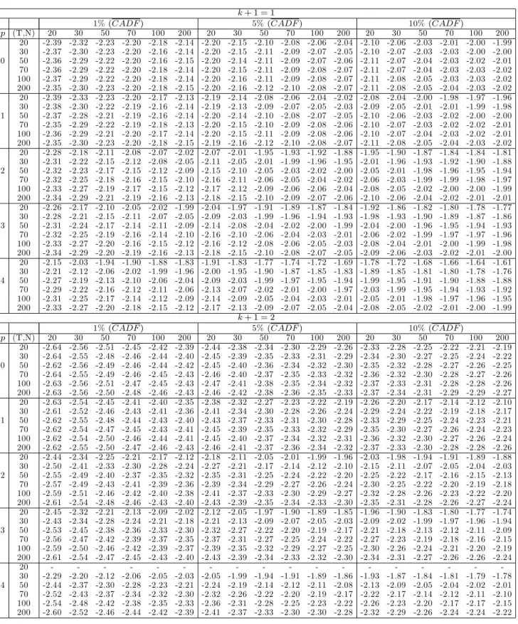
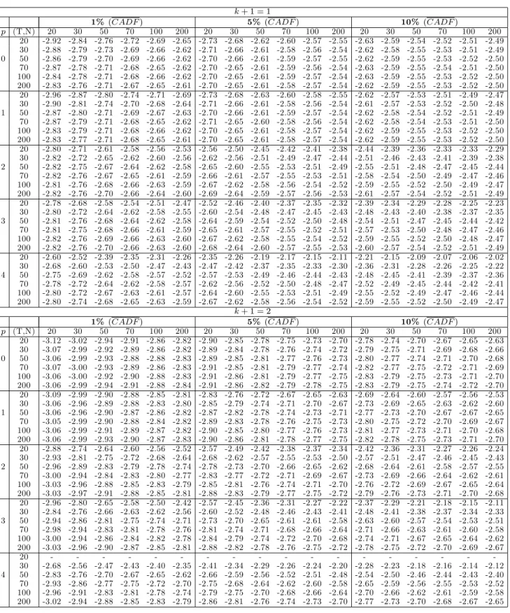
3
Critical Values
The critical values of
CADF
iand
CADF
=
N
1P
iN=1CADF
ifor di¤erent values of
k
,
N
,
T
and lag-augmentation
p
, are obtained by stochastic simulation. Based on the results in Section
2 the limit distribution of
CADF
does not depend on the factor loadings or
i. This implies
that the distribution of the test statistic is invariant to the choice of
iand
iso long as
m
k
+ 1
. Thus, without loss of generality we set
i=
=
0
, and
i=
= 1
in our stochastic
simulations.
To be more precise, the
y
itprocess is generated as
y
it=
y
it 1+
u
it,
i
= 1
;
2
; :::; N
;
t
= 1
;
2
; :::; T
,
where
u
itiidN
(0
;
1)
with
y
i0= 0
. The
j
thelement of the
k
1
vector of the additional
regressors
x
it, is generated as
x
ijt=
x
ij;t 1+
v
ijt,
i
= 1
;
2
; :::; N
;
j
= 1
;
2
; :::; k
;
t
= 1
;
2
; :::; T
,
(50)
with
v
ijtiidN
(0
;
1)
and
x
ij0= 0
. The
CADF
itest statistic is calculated as the
t
-ratio of the
coe¢ cient on
y
it 1of the regression of
y
iton
y
it 1,
z
0t 1,
(
z
0i:t 1; :::;
z
0i:t p)
,
(
z
0t 1; :::;
z
0t p)
where the following cases for the deterministics are entertained
Case I:
no deterministics,
Case II:
intercept only,
and
E
(
CADF
i)
and
V ar
(
CADF
i)
are obtained as an average over all replications of
CADF
1and
the square of the standard deviation of
CADF
1respectively, for
N; T
= 200
. The
%
critical
values of the
CADF
1and
CADF
statistics are computed for
N; T
= 20
;
30
;
50
;
70
;
100
;
200
,
k
+ 1 = 1
;
2
;
3
;
4
and
p
= 0
;
1
; :::;
4
;
as the
1
quantiles of
CADF
1and
CADF
for
=
0
:
01
;
0
:
05
;
0
:
1
. Results for the critical values of the
CADF
statistic are reported in Tables
1a-1c. The critical values for the individual statistics
CADF
iare available upon request. All
stochastic simulations are based on 10,000 replications.
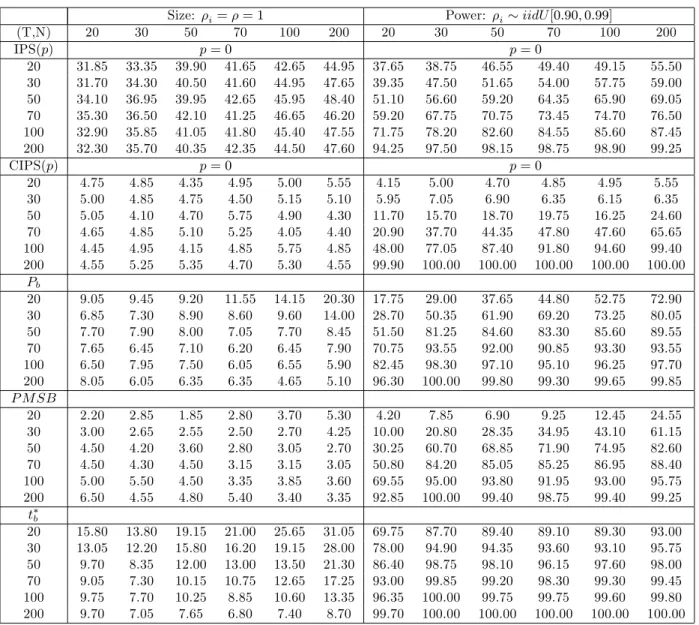
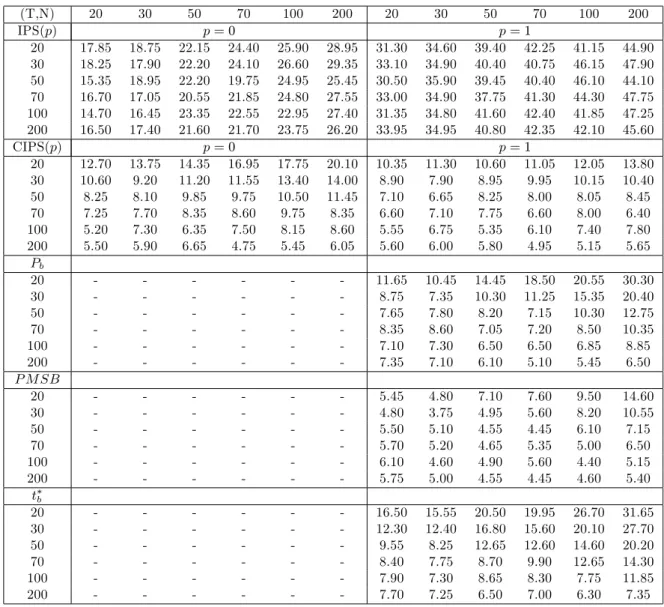
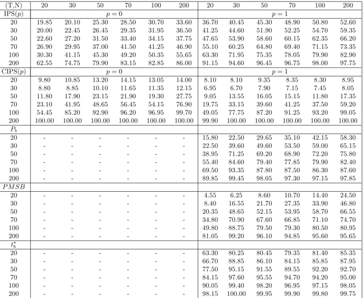
4
Small Sample Performance: Monte Carlo Evidence
In what follows we investigate the small sample properties of the CIPS test de…ned by (35)
by means of Monte Carlo experiments. Before doing so, we brie‡y present the panel unit root
test statistics that we consider in our Monte Carlo alongside the CIPS test. These include
the tests proposed by Im, Pesaran and Shin (IPS, 2003), Bai and Ng (2007), and Moon and
Perron (2004). The IPS test is not valid under cross section dependence, but is inlcuded as a
benchmark.
4.1
Alternative Panel Unit Root Test Statistics
The IPS test statistic is de…ned as
IP S
=
p
N
f
t
-
bar
N TE
(
T)
g
p
V ar
(
T)
,
where
t
-
bar
N T=
N
1P
iN=1 iT, and
iTis the t-ratio of the ADF(
p
) regression of the
i
thcross
section unit.
E
(
T)
and
V ar
(
T)
are the mean and variance of
iT, which are listed in Table 3
of Im et al (2003).
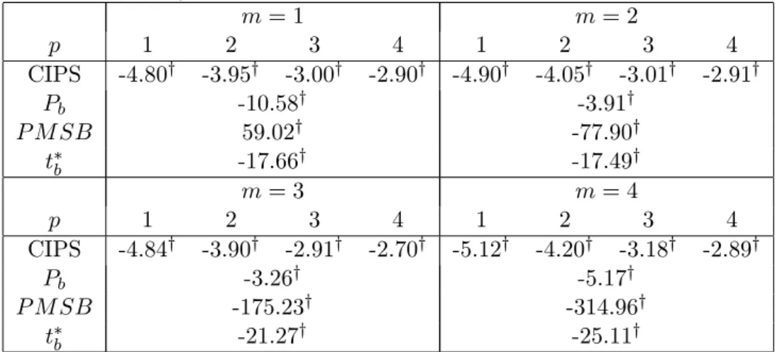
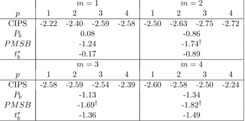
Bai and Ng (2007) propose the
P
band
P M SB
tests, both of which are brie‡y described
below. The former is the analog of the
t
bstatistic of Moon and Perron (2004) except that it
is based on a di¤erent set of residuals and the method of ‘defactoring’of the data is di¤erent,
while the latter is the panel version of the modi…ed Sargan-Bhargava test. The
P
band
P M SB
tests are based on the so called PANIC residuals, which in the context of our notation as set
out in Section 2, are obtained as follows. Firstly transform
y
it:
y
it=
y
itif
y
ithas individual
e¤ects, or
y
it=
y
ity
iwith
y
i= (
T
1)
P
Tt=2y
it, if
y
ithas a linear trend. Apply
principal components to these transformed series to estimate
F
, denoted as
F
^
, which is
p
T
1
times the
m
eigenvectors corresponding to the …rst
m
largest eigenvalues of the
(
T
1)
(
T
1)
matrix
Y Y
0, where
Y
= (
y
1
;
y
2; :::;
y
N)
and
y
i= (
y
i2; y
i3; :::; y
iT)
0
. Under the normalisation
^
F
0F
^
=
(
T
1) =
I
m, the estimated factor loadings
iare
^
i=
F
^
0iy
i=
(
T
1)
. Then obtain
^
u
it=
P
ts=2e
it, where
e
it=
y
it^
0i^
f
t.
Having obtained the PANIC residuals, the
P
btest is then based on a pooled estimate of the
autoregressive coe¢ cient
in the following regression
^
u
it= ^
u
i;t 1+
it:
(51)
The bias-corrected pooled PANIC autoregressive estimator for
u
^
itbased on OLS estimation of
^
+=
tr
(
^
U
0 1M ^
U
N T
^
)
tr
(
U
^
0 1M ^
U
1)
where
U
^
are
(
T
2)
N
matrices and
^
is the bias correction estimated from
E
^
=
M ^
U
^
M ^
U
1with
^ =
tr
(
^
U
0 1M ^
U
)
tr
(
U
^
0 1M ^
U
1)
and
M
=
I
T 2in the case of no deterministics or a constant only and
M
=
I
T 1D
(
D
0D
)
1D
0in the case of an intercept and a linear trend, where
D
= (
d
1; :::;
d
T 1)
0and
d
t= (1
t
)
0:
The
P
bstatistic is de…ned as
P
b=
p
N T
(^
+1)
v
u
u
t
1
N T
2tr
(
U
^
1M ^
U
0 1)
K
b^
!
2^
4.
(52)
The bias adjustment depends on the treatment of the deterministic terms such that in the
case of no deterministics or a constant only
( ^
; K
b) = (^
;
1)
;
and
( ^
; K
b) = ( ^
2=
2
;
4)
in the
case of an intercept and a linear trend, where
M
is de…ned as above. The parameters
^
2;
!
^
2;
^
and
^
4;
are the limits of the cross section averages of the short and long run variance, the
one-sided long run variance and the limit of the cross section averages of the square of the long
run variance, respectively.
The
P M SB
statistic is de…ned as
P M SB
=
p
N
(
tr
(
N T12U
^
0U
^
)
^
q
^
4=K
msbwhere as above the bias correction depends on the deterministic trends. In the case of no
deterministics or a constant only
( ^
; K
msb) = (^
! =
2
;
3)
;
and
( ^
; K
msb) = (^
! =
6
;
45)
in the case
of an intercept and a linear trend.
To compute the
t
btest statistic proposed by Moon and Perron (2004), initially the pooled
OLS estimator is obtained from a …rst order autoregressive model of the observed data. A factor
model is then estimated using the residuals computed based on the pooled OLS estimator and
the factor loadings are obtained. The bias-corrected defactored pooled OLS estimator is then
de…ned similar to (52) above where
U
^
is replaced by the de-factored panel data obtained by
projecting the panel data onto the space orthogonal to the (estimated) factor loadings. The
nuisance parameters are de…ned on the residuals of the defactored data where the long-run
variance is estimated by employing Andrews and Monahan’s (1992) estimator based on the
quadratic spectral kernel and prewhitening.
All the above test statistics are asymptotically distributed as standard normal so that they
all reject the null hypothesis if they are less than -1.645, at the 5% signi…cance level. For further
details see Bai and Ng (2007) and Moon and Perron (2004).
For the test procedures proposed by Bai and Ng (2007) and Moon and Perron (2004) that
require the estimation of the number of factors, information criteria proposed by Bai and Ng
(2002) are typically used, initialised by speci…cation of the maximum number of factors. In
what follows we consider experiments where the number of factors is treated as known, as well
as experiments where the number of factors are estimated. In the latter case we use the BIC3
criterion of Bai and Ng (2002) which is favoured by these authors as more robust in the presence
of cross section correlation in the idiosyncratic errors.
Finally, it is worth noting that we do not consider the
P
aand
t
atests of Bai and Ng
(2007) and Moon and Perron (2004), respectively, as these tests do not perform as well as the
alternative
P
band
t
btests.
4.2
Monte Carlo Design
Initially we shall consider dynamic panel models with …xed e¤ects and a two-factor error
struc-ture. The data generating process (DGP) is given by
y
it= (1
i)
i+
iy
i;t 1+
i1f
1t+
i2f
2t+
"
it; i
= 1
;
2
; :::; N
;
t
=
49
; :::; T
(53)
with
y
i; 50= 0
, where
iiidN
(1
;
1)
,
f
jt=
f jf
f j;t 1+
$
jt; $
jtiidN
(0
;
1)
;
(54)
with
f
j; 50= 0
and
f j= 0
for
j
= 1
;
2
;
and
"
it=
i""
it 1+
it;
itiidN
(0
;
2i)
;
(55)
with
"
i; 50= 0
and
i"=
"= 0
,
i2iidU
[0
:
5
;
1
:
5]
. The
x
itprocess is generated as
x
it=
i+
ix1f
1t+
ix2f
2t+
v
ixt; i
= 1
;
2
; :::; N
;
t
=
49
; :::; T
(56)
with
x
i; 50= 0
, where
iiidN
(1
;
1)
, and
v
ixt=
v
ixt 1+
e
ivxt; e
ivxt=
ivxe
ivx;t 1+
%
it; %
itiidN
(0
;
1)
(57)
with
v
ix; 50= 0
,
e
ivx; 50= 0
, and
ivxiidU
[0
:
2
;
0
:
4]
. The factor loadings are generated as
i1
iidU
[1
;
3]
,
i2iidU
[0
;
2]
,
ix1iidU
[0
;
2]
,
ix2iidU
[1
;
3]
, so that
E
(
i) =
2 1
1 2
;
and the rank condition (9) is satis…ed.
We consider three combinations of serially correlated errors: (A) serially uncorrelated
"
itand
f
jt(
i"=
"= 0
and
'1=
'2= 0
); (B) serially correlated
"
it(
i"iidU
[0
:
2
;
0
:
4]
whilst
'1