This is a repository copy of
Fault Diagnosis of High-speed Train Bogie Based on
Spectrogram and Multi-channel Voting
.
White Rose Research Online URL for this paper:
http://eprints.whiterose.ac.uk/142153/
Version: Accepted Version
Proceedings Paper:
Su, L, Ma, L, Qin, N et al. (2 more authors) (2018) Fault Diagnosis of High-speed Train
Bogie Based on Spectrogram and Multi-channel Voting. In: Proceedings of DDCLS 2018.
2018 IEEE 7th Data Driven Control and Learning Systems Conference, 25-27 May 2018,
Enshi, China. IEEE , pp. 22-26. ISBN 978-1-5386-2618-4
https://doi.org/10.1109/DDCLS.2018.8516061
© 2018 IEEE. This is an author produced version of a paper published in 2018 IEEE 7th
Data Driven Control and Learning Systems Conference (DDCLS). Personal use of this
material is permitted. Permission from IEEE must be obtained for all other uses, in any
current or future media, including reprinting/republishing this material for advertising or
promotional purposes, creating new collective works, for resale or redistribution to servers
or lists, or reuse of any copyrighted component of this work in other works. Uploaded in
accordance with the publisher's self-archiving policy.
[email protected] https://eprints.whiterose.ac.uk/ Reuse
Items deposited in White Rose Research Online are protected by copyright, with all rights reserved unless indicated otherwise. They may be downloaded and/or printed for private study, or other acts as permitted by national copyright laws. The publisher or other rights holders may allow further reproduction and re-use of the full text version. This is indicated by the licence information on the White Rose Research Online record for the item.
Takedown
If you consider content in White Rose Research Online to be in breach of UK law, please notify us by
Fault Diagnosis of High-speed Train Bogie Based on
Spectrogram and Multi-channel Voting
Liyuan Su1
, Lei Ma1
, Na Qin1∗
, Deqing Huang1
, and Andrew Kemp2
1Institute of System Science and Technology, School of Electrical Engineering, Southwest Jiaotong University, Chengdu 611756,
P. R. China
2School of Electronic and Electrical Engineering, University of Leeds, Leeds, LS2 9JT, UK
Abstract:Fault diagnosis of high-speed train bogie is of great importance in ensuring the safety of train operation. The multi-channel vibration signals measured at different positions on the bogies characterize the dynamics of the vehicle and contain key information describing the performance of the bogie components. However, due to the complexity and uncertainty of the signals, it is hard to extract stable features that represent the characteristics of the signals. Besides, manual selection of reliable channels is indispensable in existing works. This paper presents an ensemble of methods for fault type recognition of high-speed train bogie based on spectrogram images and voting method. First, vibration signals of bogies are transformed to spectrogram images that are then taken as the input of Random Forests (RFs). In the next, four voting methods including Plurality Voting (PV), Classification Entropy (CE), Winner Takes All (WTA), as well as a novel method we proposed using neural network (NN) is applied for combining all the channels’ classification results to give a final decision on fault type. The proposed method not only avoid complicated feature extraction procedures by using a simple transform, but also make the best of multiple channels by automatic combination. Experiments conducted on the dataset based on SIMPACK simulations have verified the efficacy of the presented method in classifying key component(s) failures, with accuracy near 100%. Further, a more complex fault state in which the components of bogies only lose their effectiveness partially, instead of fully, has been tested and analyzed, where near 90% of accuracy is achieved. These results demonstrate the high robustness of the new method.
Key Words:High-speed train, Bogie, Fault, Severities, Classification, Spectrogram, Random forest, Voting, Multi-channel
1
Introduction
With the development of high-speed railway, the achieve-ment of speed increase benefits increasing transportation de-mands. Meanwhile, the security issues related to the high speed become more vital, more and more people focus on fault diagnosis of high-speed train. Bogie is the only con-nect unit between the train body and rails, and degenerations of its key elements will seriously threaten train safety [1]. Therefore, the study of fault diagnosis on bogies is of great significance.
In recent decades, many works have been done on the clas-sification of faults based on vibration signals acquired from the sensors mounted on the train bogies. In these works, the features of the vibration signals mainly fall into two cate-gories: those extracted by traditional signal analysis methods and those learned automatically by networks. For the former case, a feature extraction and analysis frame, which com-bines the information measurement entropy theory with a time-frequency analysis method based on the physical mean-ing of the main indicatives of information measurement the-ory was proposed by N. Qin [1]. J. Zhao et al. applied Empirical Mode Decomposition (EMD) and fuzzy entropy theory in representing the features of fault signals, then used a back-propagation neural network to classify the faults [2]. For the latter case, C Guo et al. employed a DBN hierar-chical ensemble to feature extraction, then applied a Sup-port Vector Machine (SVM) a K-nearest Neighbors (KNN) algorithm and a Radial Basis Function neural network for classification, and used a series of voting strategies to get the final result [3]. H Hu et al. used a Deep Neural Net-work for the fault diagnosis [4]. All these Net-works above take
This work was financially aided by the Natural Science Foundation of China (Nos. 61603316, 61773323, 61733015, 61640310).∗Corresponding author: N. Qin, [email protected]
the vibration data as signals in the procedure of feature ex-traction. However, it is difficult to guarantee that the fault features extracted by EMD and other traditional feature ex-traction methods are stable [3].
In this work, we present a multi-channel signal classi-fication method based on spectrogram images and voting methods. Spectrogram images have been applied in many other domains of signals classification, e.g. acoustics and medicine, along with image processing methods. M Saadet al. used Scale-invariant Feature Transform of spectrogram and back-propagation artificial neural network to classify heart abnormalities from electrocardiogram [5]. D.C.Costa
et al. combined image analysis like morphology, connected components, projection profile and threshold to the speech segmentation [6]. M Mustafaet al.extracted Gray Level Co-occurence Matrix texture features from Electroencephalo-gram spectroElectroencephalo-grams and used KNN for classification [7]. J Dembski et al. used histograms of Oriented Gradients (HOG) and SVM to playback detection in automatic speaker verification systems [8]. In this paper, the data used was acquired from a software named SIMPACK with a certain train model and the track spectrum of Wuhan-Guangzhou line. The results have empirically demonstrated the stability of spectrogram features, and have shown high-effectiveness of our proposed voting method. Meanwhile, the signal-spectrogram transform largely compress the amount of orig-inal data, which accelerates the training and testing process. The rest of this paper is structured as follows. Section 2 presents the procedure of the experiments and the meth-ods involved. Section 3 presents the results of experiments, including RF classification results and final results on two datasets. The cause of different accuracies related to differ-ent channels will be analyzed, then the effectiveness of our proposed voting method will be demonstrated by comparing
with results of other voting methods. Finally, conclusions are drawn in the last section along with anticipated future work.
2
Overview of the experiments
Figure 1 shows the flow chart of experiments in this work. The original signals were firstly separated by different chan-nels, corresponding to the data acquired from sensors in-stalled in different positions on the bogie. Secondly, for the signal of each channel, spectrogram samples were ob-tained by slicing signals according to certain time duration. The input of RF classifiers were spectrogram images them-selves, which would be proved to be more effective than the HOG features. Finally, four voting methods including PV, CE, WTA and NN were applied to combine the results of all the channels and each gives a final decision of the fault type.
multi-channel signals
spectrogram images of different channels
RF classifications
several voting methods
fault type
Fig. 1: Experiment flow chart
2.1 Spectrogram and HOG features
The spectrogram is an efficient visual representation of time-varying signals which combines time and frequency domain information. The spectrogram generation procedure is as follows. Consider a discrete signalgk (k = 1, ..., K) sampled at a certain frequency.xm(m= 1, ..., M) is a seg-ment extracted fromgk, and its Discrete Fourier Transform (DFT) can be expressed by:
X=F(w⊙xm), (1) whereF denotes the DFT matrix, andxm is applied with a segmented window before DFT. If a signal is sliced into multiple segments, its spectrogram can thus be expressed by stacking all these segments,
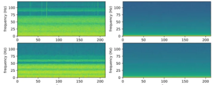
X = [X1,X2, ...,Xn]. (2) Figure 2 shows typical spectrograms of the 1st and the last (the 58th) channel for different train speeds with the same fault type, where the horizontal and vertical axis represent time and frequency respectively.
HOG feature is a image feature descriptor proposed by Dalal and Triggs [9] for object detection. Its excellent per-formance has been empirically demonstrated in pedestrian
detection, traffic sign recognition and vehicle classification. The basic idea is that local appearance and shape within an image can often be well described by the distribution of lo-cal intensity gradients or edge directions [9]. The procedure of feature extraction begins by dividing an image into spatial regions called ”cells”. In each cell, a histogram of gradi-ent directions is accumulated. Then, larger spatial regions called ”blocks” are used for the normalization of all the cells blocks. The HOG descriptor is a concatenation of feature vectors of all the blocks within an image.
Fig. 2: Spectrogram images of the same fault type (a) channel-1, 220km/s; (b) channel-58, 220km/s; (c) channel-channel-1, 140km/s; (d) channel-58, 140km/s
2.2 Random Forest
The random forest is a combination of decision trees, each of which casts a vote for the classification of a given in-stance. The decision tree is featured with simplicity, ease of use and interpretability [10], but it lacks robustness. How-ever, random forests always converge, which can be demon-strated by the strong Law of Large Numbers, therefore they do not overfit [11]. The principle of RF is bagging (boot-strap aggregation), which refers to random selections of fea-tures and training subsets while growing a tree. The bagging method decreases the correlation among trees thus guaran-teeing the immunity of RF to noise. Two main parameters in constructing a RF are the number of trees and the number of features. Once the number of trees are sufficient, the results turn out to be insensitive to the number of features selected to split each node [11], hence usually default values can pro-vide good results. The main procedure of the RF algorithm can be summarized as [12]:
i) Draw a bootstrap sample from the training set.
ii) Grow a tree by samples with certain amount of features randomly selected. For each split node, select the best split value according to a certain criterion such as Gini impurity and information gain. The tree is fully grown until no further splits are possible and it is not pruned. iii) Repeat above steps until a certain amount of trees are
grown.
The final decision of classification for an instance will be given by all the trees in the RF using the majority voting method.
2.3 Voting methods 2.3.1 Plurality Voting
PV is the most classical voting method which makes the option with the most votes the winner. Given M classi-fiers and each has a decision within {0,1,2, ..., L}. Let {m0, m1, ..., mL}be the total number of each decision, then
the final decision of PV can be written as:
y= arg max
i=1,2,..,L{mi} (3) 2.3.2 Classification Entropy
CE is a weighted voting method proposed by J Zhanget al., considering not only the total performance but also the local performance [13]. Based on the posterior probabilities provided by the training set, the algorithm involves calcu-lations of a total accuracy matrix and a local accuracy ma-trix of all classifiers. The weight mama-trixW is then calcu-lated by combining these two matrices. Each of its elements
wij stands for the weight of theithclassifier related to the
jthclass. Meanwhile,w
i,j is effected by a threshold value named ”controlling constant”. It will be enhanced if the local performance is above that value, otherwise it will be penal-ized.
2.3.3 Winner Takes All
WTA is a simple and extreme voting method. It selects the classifier with the best performance in the training proce-dure, on which the final decision will totally depend. When the performances of all classifiers vary widely, WTA can avoid the decisions of the worst classifiers.
2.3.4 Neural Network voting method
This method is an adapted method of weighted voting pro-posed by this paper. LetLbe the number of classes andM
be the number of classifiers. Then, for instance, the output of all the classifiers can be combined by aL×M matrixX, of which each elementxij satisfies
xij =
(
1 ifsj=i
0 others . (4)
sj denotes the decision of thejth classifier. The matrices are the input of the voting NN, which connects toL×M
neural nodes. The NN has only one hidden layer, with the weight matrix of each neural node related to every classifier and every class, just as the matrixW in CE; and the bias act as a correction vector. The cross entropy is used as the loss function. SGD (stochastic gradient descent) and BP (back propagation) methods are applied for updating weights and bias for obtaining an optimal network.
3
Experiments and discussion of results
3.1 Data introduction and preprocessingTwo datasets acquired from SIMPACK simulations con-sist of 58 channels. They correspond to data in different directions collected from sensors installed on different po-sitions of the bogie,e.g.train body accelerations, train struc-ture accelerations, etc. The data is recorded at a sampling frequency of 243Hz, and the total sampling time is around 3.5 mins. The two datasets differ in bogies’ health condi-tions: dataset 1 consists of one normal state and six fault types each at six running speeds. The fault types involves where one or two key components totally lose effectiveness.
Dataset 2 comprises three fault types at 11 running speeds. For each fault type, the data comprises nine different fault severities (10%, 20%, ..., 90%). More detailed descriptions of the datasets are listed in Table 1 and Table 2.
Table 1: Dataset 1 description Fault Type
#1 normal state
#2 failure of the air springs #3 failure of the lateral damper #4 failure of the anti-yaw damper
#5 failure of the air springs and the lateral damper #6 failure of the air springs and the anti-yaw damper #7 failure of the lateral damper and the anti-yaw damper speeds 40, 80, 120, 140, 160, 200 km/s
Table 2: Dataset 2 description Fault Type
#1 degeneration of air spring stiffness
#2 degeneration of secondary horizontal damping #3 degeneration of anti-yaw damping
speeds 40, 80, 120, 140, 160, 200, 220, 250, 280, 300, 350 km/s
In the preprocessing, the data was successively sliced with the duration of 3 s and an overlap of 2 s and then transformed into spectrogram images. The experiments on dataset 1 are divided into 2 parts: the faults classifications at a certain speed and with all speeds mixed, consisting of7×200 sam-ples at each speed and6×7×200samples respectively.30% and70%of the dataset was divided into the training and test-ing set for the classification stage by RF. In the vottest-ing stage, the ratio of training set, validation set and testing is2 : 1 : 2. The experiments on dataset 2 were conducted at different running speed, with each type of fault containing9×200 samples of varying degrees of degeneration of correspond-ing faulty component. Then the same division methodology with the dataset 1 was adopted for the classification and vot-ing stage.
3.2 Fault classifications with Random Forests
On dataset 1, two sets of experiments were conducted in this stage of studying the effectiveness of HOG features. The original dimension of each spectrogram sample is129×4. For the experiment using HOG features, the spectrogram im-ages were resized to64×64(resized to64, then we simply replicated each column 16 times) and normalized accord-ing to the maximum value of the trainaccord-ing dataset. In order to maintain the same data precision, for another set of ex-periments, the spectrogram images were resized to64×4. The parameters for HOG (fHOG) feature extractions [14] are listed in Table 3. The results are illustrated in Figure 3.
Table 3: Parameters of HOG feature extraction algorithm Value Description
binSize 8 spatial bin size
nOrients 9 number of orientation bins clip 0.2 value at which to clip histogram bins
Fig. 3: Results of RF classifications at different running speeds (dataset 1) (a) the difference of accuracies without and with HOG feature; (b) accuracies of results without HOG features
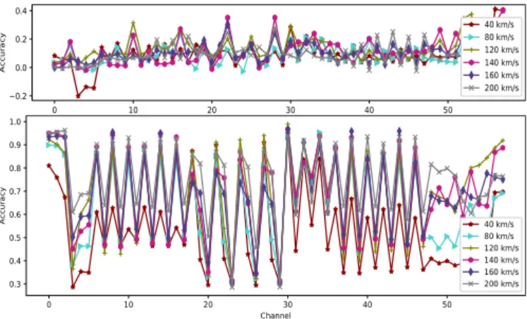
Higher classification accuracies are achieved directly us-ing spectrogram, while useful information is lost usus-ing HOG features. The difference between the results could be ex-plained by the characteristics of the spectrograms. Compar-ing to other signals such as electrocardiogram and electroen-cephalography, the spectrogram of the vibration signals for the high-speed train bogie is quite uniform along the axis of time, which means its statistical characteristics are more prominent than its spatial characteristics. It is also noticed that the accuracy of different channels varies widely. More specifically, the channels corresponding to the Y-direction signals have higher accuracies while those corresponding Z-direction signals have lower accuracies, where the Y tion is perpendicular to the railway and Z is in vertical direc-tion (and X is along the railway longitudinal direcdirec-tion) [15]. Hence, the faults of the key components of bogie are mainly reflected by the lateral vibration, which is also a main cause of hunting movement. The results also show that when the running speed is low (40 km/s in the experiments), the faults are more difficult to classify. The performances of different channels are similar at different running speeds, which con-firms the possibility of classifying faults without specified speed. In addition, the signal-spectrogram transform largely compresses the amount of data. For a single original sample of dimension243×58, its corresponding spectrogram image has only1.84%of its original dimension. This compression filters out redundant information and preserves stable fault features, which also facilitates the acceleration of the train-ing and testtrain-ing process.
Experiments were repeated on the dataset with all speeds mixed. As shown in Figure 4, the raw images still show superior performance than the HOG features.
3.3 Channel combination
For the purpose of making the best of multi-channel data, four voting methods including NN, PV, CE and WTA were adopted for combining results of all the channels. Since CE and WTA don’t need a validation set and PV requires only a testing set, to ensure fairness of comparison, those unwanted sets are discarded directly in the experiments. Experiments have been conducted 20 times with the same set of random seeds for each method to ensure the objectivity of the re-sults. In CE, the control value was set to 0.8. In NN, the
net-Fig. 4: Comparison of the RF results with/without HOG features with mixed running speeds (dataset 1)
work was set to stop training when the validation accuracy reached 100% or the number of training epochs attained 50. The batch size was 100 and the learning rate was 0.1. Re-sults are shown in Figure 5 and Table 4. Among these meth-ods, NN performs the best and is the most robust with an accuracy close to 100% even in the most complicated case where all the running speeds are mixed. The results of CE and WTA are close and acceptable, fluctuating in the range of93%∼100%. It is noticed that the results of CE are not always better than those of WTA, which indicates that CE is inferior to NN in balancing local performance and the over-all performance of classifiers. Because PV ignores the huge differences in the ability of different channels to classify, it has the lowest accuracies ranging from 79% to 96%.
Fig. 5: Final results of dataset 1
3.4 Classification with mixed fault severities
Figure 6 shows part of the results of fault type classifi-cation by RF on dataset 2. Due to the mix of fault severi-ties, even with fewer fault types, the classification accuracies are generally lower than those of dataset 1. But the high-accuracy channels stay the same, and lower speed results are still worse than higher speed.
Fig. 6: Comparison of RF results at some running speeds (dataset 2)
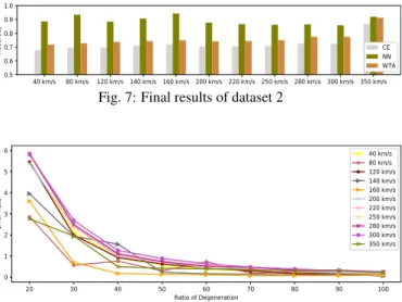
In the combination stage, results of three voting methods including NN, CE and WTA were compared. The control value was set to 0.6 in CE . In NN, the network was set to stop training after 70 epochs, and other parameters were the same as before. According to the results shown in Fig-ure 7, the performance of NN voting method is still proved
Table 4: Final results of dataset 1
speed (km/s) 40 80 120 140 160 200 all speeds mixed PV (%) 79.25 85.14 95.79 94.63 88.33 93.23 85.91 CE (%) 93.16 95.85 98.71 98.47 96.39 96.76 92.71 NN (%) 99.63 99.54 99.86 99.83 99.40 99.72 99.57 WTA (%) 94.86 95.56 99.08 96.57 96.85 96.26 94.11
to be superior to that of other methods, with an accuracy around 90%. Figure 8 illustrates the error rate of different fault severities. On the whole, with the increase of degener-ation, the classification errors decrease, since higher ratio of degeneration implies more stable fault features.
Fig. 7: Final results of dataset 2
Fig. 8: Error rate of different fault severities (dataset 2)
4
Conclusions
In this paper, an ensemble of methods of fault diagnosis of a high-speed train bogie using spectrogram images is pre-sented. It utilizes a single-layer NN voting method to com-bine multiple channels and give the final result. This method was tested on two different datasets and has been proven to have a high classification accuracy. In classifying key component(s) failure (seven fault types including one nor-mal state, three single failures and three combined failures) and faults with mixed fault severities (from 10% to 90%), high classification accuracies are achieved. However, the ac-curacy of the latter case (∼90%) is less satisfying than that of the former case (∼100%).
In future work, methods to improve the performance of the classification of mixed fault severities with more fault types will be explored. Regression models for the prediction of the degree of degeneration will be researched, to further improve the whole system of fault diagnosis of the high-speed train bogie.
References
[1] N. Qin,Research on High-Speed Train bogie fault data fea-ture analysis method based on information entropy measure-ment [D], Ph.D. thesis, Southwest Jiaotong University, 2014.
[2] J. Zhao, Y. Yang, T. Li and W. Jin, Application of empirical mode decomposition and fuzzy entropy to high-speed rail fault diagnosis, in Foundations of Intelligent Systems. Berlin, Hei-delberg: Springer, 2014: 93–103.
[3] C. Guo, Y. Yang, H. Pan, T. Li and W. Jin, Fault analysis of High Speed Train with DBN hierarchical ensemble, inNeural Networks (IJCNN), 2016 International Joint Conference on, 2017: 2552–2559.
[4] H. Hu, B. Tang, X. Gong, W. Wei and H. Wang, Intelligent fault diagnosis of the high-speed train with big data based on deep neural networks, inIEEE Transactions on Industrial In-formatics, 13(4): 2106–2116, 2017.
[5] M. Saad, M. Nor, F. Bustamiand R. Ngadiran, Classification of heart abnormalities using artificial neural network, inJournal of Applied Sciences, 7(6): 820–825, 2007.
[6] D.C. Costa, G.A.M. Lopes, C.A.B. Mello and H.O. Viana, Speech and phoneme segmentation under noisy environment through spectrogram image analysis, in Systems, Man, and Cybernetics (SMC), 2012 IEEE International Conference On, 2012: 1017–1022.
[7] M. Mustafa, M.N. Taib, Z.H. Murat and N.H.A. Hamid, GLCM texture classification for EEG spectrogram image, in
Biomedical Engineering and Sciences (IECBES), 2010 IEEE EMBS Conference on, 2010: 373–376.
[8] J. Dembski and J. Rumi´nski, Playback detection using machine learning with spectrogram features approach, inHuman Sys-tem Interactions (HSI), 2017 10th International Conference on, 2017: 31–35.
[9] N. Dalal and B. Triggs, Histograms of oriented gradients for human detection, inComputer Vision and Pattern Recognition, 2005. CVPR 2005. IEEE Computer Society Conference on, 1: 886–893, 2005.
[10] R.O. Duda, P.E. Hart and D.G. Stork,Pattern Classification, New York: Wiley, 1973.
[11] L. Breiman, Random forests, inMachine learning, 45(1): 5– 32, 2001.
[12] V. Svetnik, A. Liaw, C. Tong, J.C. Culberson, R. Sheridan and B.P. Feuston, Random forest: a classification and regres-sion tool for compound classification and QSAR modeling, in
Journal of chemical information and computer sciences, 43(6): 1947–1958, 2003.
[13] J. Zhang, Y. Wu, J. Bai and F. Chen, Automatic sleep stage classification based on sparse deep belief net and combination of multiple classifiers, inTransactions of the Institute of Mea-surement and Control, 38(4): 435–451, 2016.
[14] Piotr Doll´ar,Piotr’s Computer Vision Matlab Toolbox (PMT), https://github.com/pdollar/toolbox.
[15] W. Zhai, Z. He and X. Song, Prediction of high-speed train induced ground vibration based on train-track-ground system model, inEarthquake Engineering and Engineering Vibration, 9(4): 545–554, 2010.