Models to SMT
Ewan Davidson1, ¨Ozg¨ur Akg¨un1, Joan Espasa1, and Peter Nightingale2
1
School of Computer Science, University of St Andrews, UK
{eld5, ozgur.akgun, jea20}@st-andrews.ac.uk
2
Department of Computer Science, University of York, York, UK
Abstract. Satisfiability Modulo Theories (SMT) is a well-established methodology that generalises propositional satisfiability (SAT) by adding support for a variety of theories such as integer arithmetic and bit-vector operations. SMT solvers have made rapid progress in recent years. In part, the efficiency of modern SMT solvers derives from the use of spe-cialised decision procedures for each theory. In this paper we explore how the Essence Prime constraint modelling language can be translated to the standard SMT-LIB language. We target four theories: bit-vectors (QF BV), linear integer arithmetic (QF LIA), non-linear integer arith-metic (QF NIA), and integer difference logic (QF IDL). The encodings are implemented in the constraint modelling tool Savile Row. In an ex-tensive set of experiments, we compare our encodings for the four theo-ries, showing some notable differences and complementary strengths. We also compare our new encodings to the existing work targeting SMT and SAT, and to a well-established learning CP solver. Our two proposed en-codings targeting the theory of bit-vectors (QF BV) both substantially outperform earlier work on encoding to QF BV on a large and diverse set of problem classes.
Keywords: Constraint Modelling·SMT·Automated Reformulation
1
Introduction
Constraint programming (CP) is a powerful paradigm for solving constraint
sat-isfaction and optimisation problems, with many diverse applications.Essence
Prime [22] is a solver-independent CP modelling language that offers decision variables of Boolean and integer domains as well as arrays of these decision vari-ables, arithmetic and logical operators for expressing constraints, and global
con-straints.Essence Prime is comparable in its modelling capabilities to
MiniZ-inc [17], OPL [25], Simply [6] and other similar languages. To solve a problem
instance described in Essence Prime, a problem class model and a
parame-ter file are translated by Savile Row [21] into input suitable for a backend
solver. Savile Row applies automated reformulation steps such as common
Satisfiability Modulo Theories (SMT) is a problem solving methodology that decides the satisfiability of a propositional formula with respect to a selection of theories in first order logic with equality [20]. SMT has its roots in the field of hardware and software verification, but lately it is being used to solve a wider range of problems. The Satisfiability Modulo Theories Library (SMT-LIB) [4] provides a standard for the specification of benchmarks and theories for SMT. Most SMT solvers are restricted to decidable quantifier free fragments of their logics, which is sufficient for many applications. SMT solvers have made rapid progress in recent years. In part, the efficiency of modern SMT solvers derives from the use of specialised decision procedures for each theory. In this work we
will focus on four theories:QF LIA, QF NIA,QF IDL, andQF BV.
QF LIAandQF NIAare the theories of quantifier free linear and non-linear integer arithmetic respectively. The formulas are Boolean combinations of
con-straints comparing expressions to a constant with respect to ≤and ≥. Linear
expressions are typically enough to naturally express common problems in for-mal verification and scheduling problems. SMT solvers typically use variants of the Simplex algorithm to implement integer arithmetic theories [12].
QF IDL is the theory of quantifier free integer difference logic. It supports
Boolean combinations of inequalities of the form x−y < b where x and y
are integer variables and b is an integer constant. The renewed interest in this
fragment came from timed automata, where the verification conditions arising take the form of difference logic formulas [18].
QF BV is the theory of quantifier-free formulas over fixed-size bit-vectors. Bit-vector arithmetic is very commonly used for verification and equivalence checking in the hardware industry. Current solvers [13] typically apply heavy preprocessing techniques that ultimately flatten the formula to SAT, also known asbit-blasting.
The main contribution of this paper is a new SMT backend forSavile Row
that is able to produce any one of the four theories listed above and at two different levels of flattening, thus providing eight distinct SMT encodings. We exhaustively evaluate the performance of these encodings, showing that our en-codings perform significantly better than existing SMT approaches [9] and that
they are complementary to the existing SAT and CP backends ofSavile Row.
2
Related Work
There has been a great deal of work on translating declarative constraint mod-elling languages to lower-level languages such as SAT, SMT, and MIP. We cannot cover it all here so we cover all the most relevant work (on translation to SMT) and give examples for the rest. One example of SAT encoding is FznTini [14], which translates FlatZinc into SAT. The MiniZinc compiler is able to translate the MiniZinc language into MIP [5]. There are several encodings of a constraint language to SMT: Simply [6,8], fzn2smt [7], and FZN2OMT [9].
Simply [6] is a compiler from a custom constraint modelling language
QF IDL logics and was later extended to support meta-constraints and weighted CSPs [8]. The same authors presented fzn2smt [7], an approach that translates FlatZinc models to SMT, supporting the standard data types and constraints of FlatZinc. The logic used for solving each instance is determined automati-cally during the translation, and it handles optimisation problems by means of a dichotomic (binary) search on the domain of the optimisation variable. As in our approach, search annotations are ignored, as they do not make sense in the context of SMT. Only the allDifferent and Cumulative global constraints are supported by decomposing them into SMT.
FZN2OMT [9] can translate standard FlatZinc into suitable input for SMT solvers, and back to FlatZinc. It supports the Z3 [16] and OptiMathSAT [24] solvers, using either the QF BV or QF LIRA logics. When using OptiMathSAT, it takes advantage of the fact that OptiMathSAT natively supports a subset of the FlatZinc 1.6 language. Unlike fzn2smt, FZN2OMT is compatible with the current MiniZinc toolchain. We compare our proposed SMT encodings to all four configurations of FZN2OMT in Section 4 below.
3
Translating Essence Prime to SMT
The modelling toolSavile Rowworks by reading a problem class model written
inEssence Primeand optionally a parameter file that contains values defining a problem instance. It instantiates the problem class model, unrolls
comprehen-sions and quantified exprescomprehen-sions, and performs expression flattening where the
target solver language does not support nested expressions. Flattening is the task
of introducingauxiliaryvariables to represent nested subexpressions. Section 3.3
explains flattening in the SMT backend.
The input to Savile Row is a solver-independent model with nested
ex-pressions.Savile Rowalready has existing backends to several CP/SAT/MIP
solvers, some of these via FlatZinc. Some of these backends require a lower level output than others. For example, Minion’s input language allows a limited form of nesting (for example, constraints may be contained in conjunctions and disjunctions) but still requires a mostly flat structure, whereas FlatZinc-based solvers do not allow this kind of nesting at all. SMT-LIB allows more kinds of
nested expressions than any otherSavile Rowbackend. We implement a
fully-flat variant as well as anested variant that only flattens when strictly necessary.
It is difficult to know which variant will perform better for a given theory, SMT solver and problem class. Flattening introduces potentially useful new variables, and preserving nesting gives solvers access to the high-level structure.
A model in Essence Prime consists of three main components: decision
variable declarations, constraint expressions, and an optional objective function. The following sections explain how these components are translated to SMT.
3.1 Decision Variables and Their Domains
Essence Prime is a finite-domain language, where every decision variable is
integers as atomic types, and matrices of arbitrary dimensions of these atomic
types. Savile Row expands matrices to lists of atomic types so its output
languages do not need to support matrices or arrays. For example, given a matrix
M with three rows and columns, it will create 9 declarationsM1,1,M1,2, . . .M3,3
of its declared type.
When targeting SMT, decision variable declarations are translated to their equivalent variable declarations in SMT-LIB together with unary constraints to define the bounds of the domain. For example, when using the LIA encoding, a
find x : int(1..10)declaration would be translated as the SMT integer
vari-ablexand the constraint 1≤x≤10. When using the QF BV theory, numerical
variables are represented using fixed-size signed bit-vectors (i.e. binary numbers in two’s-complement). We use as few bits as we can, governed by the largest
do-main value in the union of all decision variables.Savile Rowperforms domain
shaving by enforcing a strong level of consistency (Singleton Arc Consistency on the bounds of the variables) via Minion. This step helps in removing any unnecessarily large values in the domains and reducing the number of variables required after bit-blasting [15].
3.2 Constraints and the Objective
Constraint expressions are at the heart of a constraint model. We translate them to SMT-LIB using specialised implementations per expression type and by falling
back to the standard SAT encodings available inSavile Row where necessary.
Boolean expressions (∧,∨,→, . . . ) and relational operators over integers (<,≤, =, . . . ) are translated to use the corresponding operators in SMT-LIB.
Arith-metic operators (+, −, /, mod, abs, . . . ) are similarly translated depending on
the theory we use. Quantified expressions, such as the universally and
existen-tially quantified expression or quantified sums are unrolled and turned into ∧,
∨, and weighted sums. AllDifferent and Global Cardinality (GCC) are
decom-posed: for each value (or each constrained value in GCC) a linear constraint is used to restrict the number of occurrences of the value. Table constraints use the Bacchus encoding [3] and short tables are encoded similarly [1].
SMT solvers are typically implemented by augmenting an existing SAT solver with implementations of theories. Hence, they allow SAT clauses in the input. We implement our SMT encodings when they are specifically supported by a
backend theory and fall back to the existing SAT encodings inSavile Rowfor
the rest of the cases.
When targeting the QF BV logic, we usebvadd,bvor andbvnegas
appropri-ate for arithmetic and logical expressions. These operators are not restricted to linear expressions, they support nested expressions with sums, multiplications, divisions, and modulo operations. Modern QF BV solvers typically use a tech-nique called bit-blasting (amongst others). Bit-blasting converts the problem to SAT by introducing a SAT variable for each bit in a bit vector. This approach can generate a smaller encoding when compared to the direct or order
encod-ings used by the SAT backend of Savile Row[23], since the direct and order
The objective function (if present) is represented by a single decision variable and dichotomic search is applied to find the optimal solution. However, when Z3 is the target solver we use its built-in optimisation (regardless of the theory). In our experiments we use Z3 for QF NIA and other solvers for the other three theories, so solver built-in optimisation is only used with QF NIA.
3.3 Flat vs Nested Encodings
Essence Prime(like MiniZinc, OPL and other comparable constraint modelling
languages) allows statingnested constraints such as allDiff([x+ 1, y+ 2, z+ 3]) directly. This constraint is considered nested because each element of the list inside the allDiff constraint is an expression and not a decision variable.
Some of the backend solvers for Savile Row do not support nested
con-straints, and therefore constraints like these have to be flattened. In this case,
the flattening process would create auxiliary variables for each sub-expression
(aux1, aux2, aux3), post additional constraints aux1 = x+ 1, aux2 =y+ 2,
aux3 =z+ 3, and replace the constraint with allDiff([aux1, aux2, aux3]). This
transformation will introduce additional variables and constraints.
Since SMT-LIB allows nested expressions we have an opportunity to evaluate
the effect of usingSavile Row’s standard flattening process vs maintaining the
nested expressions and letting the SMT solver flatten them if needed. A nested encoding is likely to be smaller in size and may allow the SMT solver to do a better job if and when it chooses to flatten. We evaluate flat and nested encodings for each of the four theories in Section 4.
4
Empirical Evaluation
In this section we compare our set of encodings (Savile Row-SMT, orSR-SMT)
with the state of the art on a wide range of problems, showing the advantages of
our approach. We compare SR-SMT to the SAT encoding implemented inSavile
Row[21] using the SAT solver CaDiCaL 1.3.0, and also to the well-established
learning constraint solver Chuffed 0.10.3. In each experiment we use the same
large set of problem instances and the same basic settings of Savile Row. We
have not been able to compare our approach to fzn2smt [7] or FznTini [14], as they have become obsolete due to changes in the FlatZinc language. We compare our approach to FZN2OMT [9], described in Section 2.
SR-SMT has eight configurations and FZN2OMT has four, which presents a challenge when attempting to compare the two systems. We resolve this by using the virtual best solver (VBS) approach for each system; i.e. for each problem instance the best configuration is selected. We also look into which configurations are contributing most to the VBS for each system.
4.1 Experimental Setup
As SR-SMT outputs standard SMT-LIB2 files, we are able to target many solvers easily. For the QF LIA and QF IDL encodings we use Yices 2.6.2 [11], for the
QF BV encoding we target Boolector 3.2.1 [19] and finally for QF NIA we use Z3 4.8.8 [16]. Experience of using SMT solvers for planning and scheduling problems (expressed in QF LIA or QF IDL) led us to use Yices for those theories; Boolec-tor is known to perform well on QF BV; and Z3 was chosen for QF NIA because of its advanced preprocessing and heuristics (for example, as noted below, Z3 converts the QF NIA Discrete Tomography problem into QF BV). Regarding optimisation, we handle it by means of a binary search on the domain of the variable to optimise. The only exception is when the Z3 solver is used, as it has native support for optimisation.
The set of problem classes used is an expanded version of the one used in [21],
with 63 problem classes and 757 instances in total3. Both satisfaction and
op-timization problems are included, and opop-timization problems are reported as solved when optimality of the last solution has been proven.
We used a time limit of 1 hour total time (i.e.Savile Rowtime plus solver
time). We use PAR2 to summarise the performance of each configuration. PAR2 is the mean of total time, where the instances that timed out are assumed to have taken two times the time limit (i.e. 2 hours). Configurations with a lower PAR2 score are considered to be better.
The default set of optimisations inSavile Row are used for all solvers and
encodings: domain filtering, variable unification, aggregation and active CSE
[21]. A standard FlatZinc backend was added to Savile Row to be used for
experiments with FZN2OMT. Decompositions of global constraints closely follow
those in the MiniZincstdlibrary. For example, allDifferent is decomposed into a
clique of pairwise not-equal constraints, and global cardinality into one sum for each constrained value. The existing Chuffed FlatZinc backend is very similar but does not decompose allDifferent or lexicographic ordering constraints.
4.2 Comparison to FZN2OMT
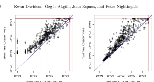
Figure 1 gives an overview of the results comparing the SR-SMT virtual best solver (SR-SMT-VBS) to the FZN2OMT virtual best solver (FZN2OMT-VBS). For SR-SMT-VBS, 685 instances were solved and for FZN2OMT-VBS 643 were solved. In Table 1 we report the number of instances solved by the two virtual best solvers as well as each configuration of both systems. The results show a clear advantage for SR-SMT-VBS on the bulk of the instances. However, there are confounding factors. First, SR-SMT-VBS is constructed from 8 configurations rather than 4, potentially giving it an advantage. Second, different SMT solvers are used. For example, Boolector was used to solve QF BV encodings in SR-SMT-VBS, whereas Z3 and OptiMathSAT were used in FZN2OMT.
Many problem classes contain the allDifferent constraint. For these, SR-SMT uses a decomposition where each value is constrained to have at most one
occur-rence using a linear constraint (in common withSavile Row’s SAT backend),
whereas the standard FlatZinc backend used with FZN2OMT decomposes to pairwise not-equal constraints. We compare the two decompositions below.
3
Experiment scripts, model and parameter files and raw results can be found at:
● ● ●●● ●● ● ●● ● ● ● ● ●●●● ● ● ● ● ● ● ● ● ● ● ● ● ● ● ● ● ● ● ● ● ● ● ● ● ● ● ●● ●● ●● ● ●● ● ● ● ● ● ● ●● ● ● ● ● ● ● ● ● ● ●● ● ● ●● ● ● ● ●●● ●● ● ●● ● ● ● ●●●● ● ● ● ●● ● ● ●● ● ● ● ● ● ● ● ● ● ● ● ● ●● ● ● ● ● ● ● ● ● ● ● ● ● ● ● ● ● ● ● ●●● ● ●●● ● ● ● ●● ●● ● ● ● ● ● ● ● ● ● ● ● ● ● ● ● ● ● ● ● ● ● ● ● ● ● ● ● ● ● ● ● ● ● ● ●● ● ● ● ● ● ● ● ● ● ● ● ● ● ● ● ● ● ● ● ● ● ● ● ● ●● ● ● ● ● ● ● ● ●●● ●● ● ● ● ● ● ● ● ● ● ● ● ● ● ● ● ● ●● ● ● ● ● ● ● ● ● ● ● ● ● ● ● ● ● ● ● ● ● ● ● ● ● ● ● ●●● ●●● ●●●● ● ● ● ●●●●● ● ● ● ● ● ● ●●●● ● ● ●●●●●●●●●●●●● ● ●●● ● ● ● ● ● ● ● ● ● ● ● ● ● ● ● ● ● ● ● ● ● ● ● ● ● ●● ● ● ● ● ● ● ● ● ● ● ● ●● ● ● ● ● ● ● ● ● ● ● ● ● ● ● ● ● ● ● ● ● ● ● ● ● ● ● ●● ● ● ● ● ● ● ● ● ● ● ● ● ● ● ● ● ● ● ●● ● ● ● ● ● ● ● ● ● ● ●● ● ● ● ● ● ● ● ● ● ● ● ● ● ● ●●●● ● ● ● ● ● ● ● ● ● ● ●● ●● ● ● ● ● ● ● ● ● ● ● ● ● ●● ● ● ● ● ● ● ● ● ● ●● ● ● ●● ● ● ● ● ● ● ● ●● ● ●●● ● ● ● ●● ● ● ●● ● ● ● ● ● ● ● ● ● ●● ● ● ● ● ● ● ● ● ●● ● ● ● ● ● ● ● ● ● ● ● ● ● ● ● ● ● ● ● ● ● ● ● ● ● ● ● ● ● ● ● ● ● ● ● ● ● ● ●● ● ● ● ● ●● ● ● ● ● ● ● ● ● ● ● ● ● ● ● ● ● ● ● ● ● ● ● ● ● ● ● ● ● ● ● ● ● ● ● ● ● ● ● ● ● ● ● ● ● ● ● ● ● ● ● ● ● ●●● ● ● ● ● ● ● ● ● ● ● ● ● ● ● ● ●●● ● ● ● ● ● ● ● ● ● ● ● ● ●●● ● ● ● ● ● ● ●● ● ● ● ● ● ● ● ● ● ● ● ● ● ● ● ● ● ● ● ● ● ● ● ● ● ● ● ● ● ● ● ● ● ● ●● ● ●●●● ● ● ● ● ●● ● ● ● ● ● ● ● ● ● ● ● ● ● ● ● ● ● ● ● ● ● ● ● ● ● ● ● ● ● ● ● ● ● ● ● ● ● ● ● ● ● ●
1e−03 1e−01 1e+01 1e+03
1e−03 1e−01 1e+01 1e+03 Solver Time SR−SMT−VBS Solv er Time FZN2OMT−VBS ● ●● ●● ●● ●● ● ● ● ● ● ●● ●● ● ● ● ● ● ● ● ●● ● ● ● ● ● ● ● ● ● ● ● ● ● ● ● ● ● ●● ●● ●● ● ●● ● ● ● ● ● ● ●● ● ● ● ● ● ● ● ● ● ●● ● ● ●● ● ● ● ● ● ●●● ● ●● ● ● ● ●● ●● ● ● ● ● ● ● ●●● ●●●●●● ● ● ● ● ● ● ●● ● ● ● ● ● ● ● ● ● ● ● ● ● ● ● ● ● ●●●● ● ● ●● ●● ● ●●●● ● ● ●● ● ● ● ● ●● ● ● ● ● ● ● ●● ● ● ● ● ● ● ● ● ● ● ● ● ● ● ● ● ● ● ● ● ● ● ● ● ● ● ● ● ● ● ● ● ● ● ● ● ● ● ● ● ● ● ● ● ● ● ● ●●●●●●● ● ● ● ● ● ● ● ● ● ● ● ● ● ● ● ● ● ● ●● ● ● ● ● ● ● ● ● ● ● ● ● ● ● ● ● ● ● ● ● ● ● ● ● ● ●●●● ●●● ●● ●● ● ● ● ●●●●● ● ● ● ●● ● ● ● ●● ● ● ●●●●●●●●●●●●● ● ● ●●● ● ● ● ● ● ● ● ● ● ● ● ● ● ● ● ● ● ● ● ● ● ● ● ● ●●● ● ● ● ● ● ● ● ● ● ● ● ●● ● ● ● ● ● ● ● ● ● ● ● ● ● ● ● ● ● ● ● ● ● ● ● ● ● ● ●●● ● ● ● ● ● ● ● ● ● ● ● ● ● ● ● ● ● ●● ● ● ● ● ● ● ● ● ● ● ●●● ● ●● ● ● ● ● ● ● ● ●●●●●●● ● ● ● ● ● ● ● ●● ● ●● ● ● ● ● ● ● ● ● ●●●● ●●●● ● ● ● ● ● ● ● ●●● ● ●● ●● ●● ● ● ●●●●● ● ● ● ●●● ●●● ● ● ●● ● ● ●● ● ● ● ● ● ● ● ● ● ●● ● ● ● ● ● ●●●●● ● ● ● ● ● ● ● ● ● ● ● ● ● ● ● ● ● ● ● ● ● ● ● ● ● ● ● ● ●● ● ● ● ● ● ●●●●●●● ● ● ● ● ● ● ● ● ● ● ● ● ● ● ● ● ● ● ● ● ● ● ● ● ● ● ● ● ● ● ● ● ● ● ● ● ● ● ● ● ● ● ● ● ● ● ● ●● ● ● ● ● ● ● ● ● ● ●●● ● ● ● ● ●● ● ●● ●● ● ● ● ● ●●● ● ● ● ● ● ● ● ● ● ● ● ● ● ● ● ● ● ● ● ● ● ●● ● ● ● ● ● ● ● ● ● ● ● ● ● ● ● ● ● ● ● ● ● ● ● ● ● ● ● ● ● ● ● ● ● ●●● ● ●●●● ● ● ● ● ●● ● ● ● ● ● ● ●●● ● ● ● ●● ● ●● ● ● ● ● ● ● ● ● ● ● ● ● ● ● ● ● ● ● ● ● ● ● ● ● ● ●
1e−01 1e+00 1e+01 1e+02 1e+03
1e−01 1e+00 1e+01 1e+02 1e+03 Total Time SR−SMT−VBS T
otal Time FZN2OMT−VBS
Fig. 1: SR-SMT-VBS vs FZN2OMT-VBS, solver time (left) and total time (right).
Encoding Instances solved Mean PAR2
SR-SMT-VBS 685 803 SR-SMT-Nested-VBS 682 840 SR-SMT-Flat-VBS 682 839 FZN2OMT-VBS 643 1283 SR-SMT-BV-Nested 663 1092 SR-SMT-BV-Flat 661 1106 SR-SMT-NIA-Nested 499 2620 SR-SMT-NIA-Flat 511 2522 SR-SMT-LIA-Nested 590 1695 SR-SMT-LIA-Flat 586 1729 SR-SMT-IDL-Nested 592 1714 SR-SMT-IDL-Flat 591 1716 SR-SMT-BV-Nested-Z3 657 1138 SR-SMT-BV-Nested-Z3-PA 643 1228 FZN2OMT-LIA-Z3 508 2638 FZN2OMT-LIA-OptiMathSAT 517 2609 FZN2OMT-BV-Z3 587 1921 FZN2OMT-BV-OptiMathSAT 533 2454 SAT 671 931 Chuffed 637 1248
Table 1: Number of instances solved and PAR2 for each configuration. Bold indicates the overall best configuration (by instances solved), red indicates the best configuration of one system (SR-SMT or FZN2OMT).
● ● ●●● ●● ●● ● ● ● ● ● ● ● ● ● ● ● ● ● ● ● ● ● ● ● ● ● ● ● ● ● ● ● ● ● ● ● ● ● ● ● ●● ●● ●● ● ●● ● ● ● ● ● ● ●● ● ● ● ● ● ● ● ● ● ●● ● ● ●● ● ● ● ●●● ●● ● ●● ● ● ● ●● ●● ● ● ●●●● ●●● ● ● ● ● ● ● ● ● ● ● ● ● ● ● ● ● ● ● ● ● ● ● ● ● ● ● ● ● ● ● ● ● ●●●●● ● ● ●● ● ● ●●● ● ● ● ● ● ● ● ● ● ● ● ● ● ● ● ●● ● ● ● ● ● ● ● ● ● ● ● ● ● ● ● ● ● ● ● ● ● ● ● ● ● ● ● ● ● ● ● ● ● ● ● ● ● ● ● ● ● ● ● ●● ● ● ● ● ● ● ● ●●● ● ● ● ● ● ● ● ● ● ● ● ● ● ● ● ● ● ● ● ● ● ● ● ● ● ● ● ● ● ● ● ● ● ● ● ● ● ● ● ● ● ● ● ● ●●●●● ●●●●●●● ● ● ● ●●●● ● ● ● ● ● ● ● ●●●● ● ● ●●●●●●●●●●●●● ● ● ●●● ● ● ● ● ● ● ● ● ● ● ● ● ● ● ● ● ● ● ● ● ● ● ● ● ● ●● ● ● ● ● ● ● ● ● ● ● ● ●● ● ● ● ● ● ● ● ● ● ● ● ● ● ● ● ● ● ● ● ● ● ● ● ● ● ● ●● ● ● ● ● ● ● ● ● ● ● ● ● ● ● ● ● ● ● ●● ● ● ● ● ● ● ● ● ● ● ●● ● ● ● ● ● ● ● ● ● ● ● ● ● ●●●●● ● ● ● ● ● ● ● ● ● ● ●● ●● ● ● ● ● ● ● ● ● ● ● ● ● ●● ● ● ● ● ● ● ● ● ● ● ● ●● ●● ●● ● ● ● ● ● ● ● ● ● ●● ● ●●● ● ● ● ●●● ● ●● ● ● ● ● ● ● ● ● ● ●● ● ● ● ● ● ● ● ● ●● ● ● ● ● ● ● ● ● ● ● ● ● ● ● ● ● ● ● ● ● ● ● ● ● ● ● ● ● ●● ● ● ● ● ● ● ● ● ● ● ● ● ● ● ● ● ●● ● ● ● ● ● ● ● ● ● ● ● ● ● ● ● ● ● ● ● ● ● ● ● ● ● ● ● ● ● ● ● ● ● ● ● ● ● ● ● ● ● ● ● ● ● ● ● ● ● ● ● ● ●●● ● ● ● ● ● ● ● ● ● ● ● ● ● ●● ●●● ● ● ● ● ● ● ● ● ● ● ● ● ●●● ● ● ● ● ● ● ●● ● ● ● ● ● ● ● ● ● ● ● ● ● ● ● ● ● ● ● ● ● ● ● ● ● ● ● ● ● ● ● ● ● ● ●● ● ●●●● ● ● ● ● ●● ● ● ● ● ● ● ● ● ● ● ● ● ● ● ● ● ●● ● ● ● ● ● ● ● ● ● ● ● ● ● ● ● ● ● ● ● ● ● ● ● ● ●
1e−03 1e−01 1e+01 1e+03
1e−03
1e−01
1e+01
1e+03
Solver Time SR−SMT−Flat−VBS
Solv er Time FZN2OMT−VBS ● ● ●●● ● ● ●● ● ● ● ● ● ●●●● ● ● ● ● ● ● ● ●● ● ● ● ● ● ● ● ● ●● ● ● ● ● ● ● ● ●● ●● ●● ● ●● ● ● ● ● ● ● ●● ● ● ● ● ● ● ● ● ● ●● ● ● ●● ● ● ● ● ● ●●● ● ●● ● ● ● ●● ●● ● ● ●●●● ● ● ● ●●●●●● ● ● ● ● ● ● ●● ● ● ● ●● ● ● ● ● ● ● ● ● ● ● ● ● ●●●● ● ● ●● ●● ● ●● ●● ● ● ●● ● ● ● ● ●● ● ● ● ● ● ●●● ● ● ● ● ● ● ● ● ● ● ● ● ● ● ● ● ● ● ● ● ● ● ● ● ● ● ● ● ● ● ● ● ● ● ● ● ● ● ● ● ● ● ● ● ● ● ● ●●●●●●● ● ● ● ● ● ● ● ● ● ● ● ● ● ● ● ● ● ● ● ● ● ● ● ● ● ● ● ● ● ● ● ● ● ● ● ● ● ● ● ● ● ● ● ● ●●●●● ●●●●●●● ● ● ● ●●●● ● ● ● ● ●● ● ●● ●● ● ● ●●●●●●●●●●●●● ● ● ●● ● ● ● ● ● ● ● ● ● ● ● ● ● ● ● ● ● ● ● ● ● ● ● ● ● ●●● ● ● ● ● ● ● ● ● ● ● ● ●● ● ● ● ● ● ● ● ● ● ● ● ● ● ● ● ● ● ● ● ● ● ● ● ● ● ● ● ● ● ● ● ● ● ● ● ● ●● ● ● ● ● ● ● ● ● ●● ● ● ● ● ● ● ● ● ● ● ●● ● ● ●● ● ● ● ● ●● ● ●●●●●●● ● ● ● ● ● ● ● ●●● ● ●● ● ● ● ● ● ● ● ●●●● ●● ●● ● ● ● ● ● ● ● ●●● ● ●● ● ● ●● ● ● ●●●●●● ● ● ●●● ●●● ● ● ●● ● ● ● ●● ● ● ● ● ● ● ● ● ●● ● ● ● ● ● ●●●●● ● ● ● ● ● ● ● ● ● ● ● ● ● ● ● ● ● ● ● ● ● ● ● ● ● ● ● ● ●● ● ● ● ● ● ●●●●●●● ● ● ● ● ● ● ● ● ● ● ● ● ● ● ● ● ● ● ● ● ● ● ● ● ● ● ● ● ● ● ● ● ● ● ● ● ● ● ● ● ● ● ● ● ● ● ● ●● ● ● ● ● ● ● ● ● ● ●●● ● ● ● ● ●● ● ●● ●● ● ● ●● ●●● ● ● ● ● ● ● ● ● ● ● ● ● ● ● ● ● ● ● ● ● ● ●● ● ● ● ● ● ● ● ● ● ● ● ● ● ● ● ● ● ● ● ● ● ● ● ● ● ● ● ● ● ● ● ● ● ●●● ● ●●●● ● ● ● ● ●● ● ● ● ● ● ● ●●● ● ● ● ●● ● ●● ● ● ● ● ● ● ● ● ● ● ● ● ● ● ● ● ● ● ● ● ● ● ● ● ● ●
1e−01 1e+00 1e+01 1e+02 1e+03
1e−01
1e+00
1e+01
1e+02
1e+03
Total Time SR−SMT−Flat−VBS
T
otal Time FZN2OMT−VBS
Fig. 2: SR-SMT-Flat-VBS (i.e. virtual best solver of the 4 Flat configurations) vs FZN2OMT-VBS, solver time (left) and total time (right).
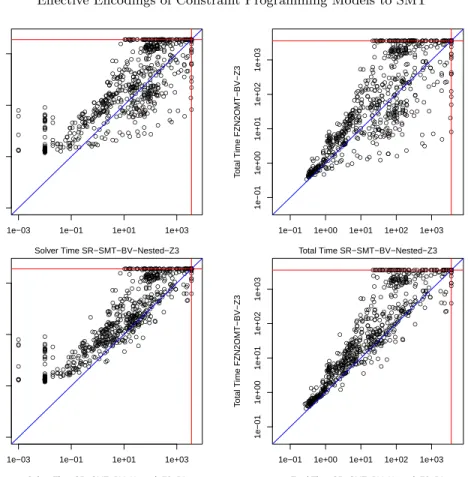
To provide a fairer comparison between two portfolios of the same size, we constructed two further virtual best solvers for SR-SMT, one using the four Flat configurations (SR-SMT-Flat-VBS) and the other using the four Nested configu-rations (SR-SMT-Nested-VBS). As Table 1 shows, the Flat configuration solves more instances for one theory (QF NIA) and is quite close to Nested in perfor-mance for the other theories. On the other hand, Nested solves more instances with the most promising theory (QF BV) and also QF LIA and QF IDL. It turns out that SR-SMT-Flat-VBS is very slightly stronger (Table 1). Figure 2 com-pares SR-SMT-Flat-VBS to FZN2OMT-VBS, and Table 1 contains the number of instances solved and PAR2 score for both. Even with a smaller portfolio it is clear that SR-SMT is performing better than FZN2OMT on these benchmarks. Also, there is the issue that the solvers do not match for any theory. SR-SMT uses Yices with QF LIA and Boolector with QF BV, whereas FZN2OMT uses Z3 and OptiMathSAT. To be able to compare just the encodings, we ran SR-SMT-BV-Nested (the strongest configuration of SR-SMT measured by instances solved and PAR2) with Z3 instead of Boolector, creating a configuration called SR-SMT-BV-Nested-Z3. Table 1 shows that SR-SMT-BV-Nested-Z3 is somewhat weaker than SR-SMT-BV-Nested on these benchmarks, solving 6 fewer instances within 1 hour and having a higher PAR2 score. Figure 3 compares SR-SMT-BV-Nested-Z3 to FZN2OMT-BV-Z3. The results are mixed, with some instances solving much faster with BV-Z3, and 15 solved only by FZN2OMT-BV-Z3. However, the overall trend is that SR-SMT-BV-Nested-Z3 is stronger, it solves 70 more instances and has a lower PAR2 score.
Finally, there is the issue that the decompositions of AllDifferent do not match. We created another configuration SR-SMT-BV-Nested-Z3-PA, which is SR-SMT-BV-Nested-Z3 with the pairwise decomposition of AllDifferent (match-ing FZN2OMT). As Table 1 shows, the new configuration is weaker than
SR-● ● ● ● ● ● ●●● ● ● ● ● ● ● ● ● ● ● ● ● ● ● ● ●● ● ● ● ● ● ● ● ● ● ● ● ● ● ● ● ● ● ● ●● ●● ● ● ● ● ● ● ● ● ● ● ● ● ● ●● ● ● ● ● ● ● ● ●● ● ● ● ● ● ● ● ●● ● ● ● ● ● ●● ● ● ● ●● ●● ● ● ●● ● ● ●● ● ● ● ● ● ● ● ●● ● ● ● ●● ● ● ● ●● ● ● ● ● ● ● ● ● ●● ● ● ● ● ●●● ● ● ● ●● ● ●● ● ●● ● ● ● ● ● ● ● ● ● ●● ● ● ● ● ● ● ●● ● ●● ● ●●●● ● ● ● ● ● ● ● ● ● ● ●●●● ● ● ● ● ● ●●● ● ● ●●● ●● ● ● ● ● ● ● ● ● ● ● ● ● ● ● ● ● ● ● ● ●● ● ● ● ● ● ● ● ● ● ● ● ● ● ● ● ● ● ● ● ● ● ● ●●●● ● ● ● ● ● ● ● ● ● ● ● ● ● ● ●●●● ●● ●●●●●●● ●●●● ● ● ●● ●● ● ● ● ●●●●●●●●●●●●●●●●● ● ● ● ●● ● ● ● ● ● ● ● ● ● ● ● ● ● ● ● ● ● ● ●● ● ● ● ● ● ●● ● ● ● ● ● ● ● ● ● ● ● ●● ● ● ● ● ● ● ● ● ● ● ● ● ● ● ● ● ● ● ● ● ● ● ● ● ● ● ● ● ● ● ● ● ● ● ● ● ● ● ● ● ● ● ● ● ● ● ● ● ● ● ● ● ● ● ● ● ● ● ● ● ● ● ● ● ● ● ● ● ● ● ● ● ● ● ● ●● ● ● ● ● ● ● ● ● ● ● ● ● ● ● ● ● ● ● ● ● ● ● ● ● ● ● ● ● ● ● ● ● ● ● ● ● ● ● ● ● ● ● ● ● ● ● ● ● ● ● ● ● ● ● ● ● ●● ●●● ●● ● ● ● ● ● ● ● ● ● ● ● ● ● ● ● ● ● ● ● ● ● ● ● ● ● ● ●● ● ● ● ● ● ● ● ● ● ● ● ● ● ● ● ● ● ● ●● ● ● ● ● ● ● ● ● ● ● ● ● ● ● ● ● ● ● ● ● ● ● ● ● ● ● ● ● ● ● ●● ● ● ● ● ● ● ● ● ● ● ● ● ● ● ● ● ● ● ● ● ● ● ●● ● ● ● ● ●● ● ● ● ● ● ● ● ● ● ● ● ● ● ● ●● ● ●●●● ● ● ● ● ●● ● ● ● ● ● ● ● ● ● ● ● ● ● ● ● ● ● ● ● ● ● ● ● ● ●●● ● ● ●● ● ● ● ● ● ● ● ● ● ● ● ● ● ● ● ● ● ● ● ● ● ● ● ● ● ● ● ● ● ● ● ● ● ●● ● ● ●● ●●●●●● ● ● ● ● ● ●● ● ● ● ● ● ● ● ● ● ● ●● ● ●●● ● ● ● ● ● ● ● ● ● ● ● ● ● ● ● ● ● ● ● ● ● ● ● ●●●
1e−03 1e−01 1e+01 1e+03
1e−03
1e−01
1e+01
1e+03
Solver Time SR−SMT−BV−Nested−Z3
Solv er Time FZN2OMT−BV−Z3 ● ● ● ● ● ● ● ●● ● ● ● ● ● ●● ●● ● ● ● ● ● ● ● ● ● ● ● ● ● ● ● ● ● ● ● ● ● ● ● ● ● ● ●● ● ● ● ● ● ● ● ● ● ● ● ● ● ● ● ●● ● ● ● ● ● ● ● ●● ● ● ● ● ● ● ● ●● ● ● ● ● ● ●● ● ● ● ●● ●● ● ● ●● ● ● ● ● ●●●●●● ● ●● ● ● ● ●● ● ● ● ●● ● ● ● ● ● ● ● ● ●●● ● ● ● ● ●● ● ● ●●● ● ● ● ● ● ● ● ● ● ● ● ● ● ● ● ●● ● ●● ● ● ● ●● ● ●● ● ●●●● ● ● ● ●● ● ● ● ● ● ● ●● ● ● ● ● ● ● ●● ● ● ● ● ● ●● ● ● ● ● ● ● ● ● ● ● ● ● ● ● ● ● ● ● ● ● ●● ● ● ● ● ● ● ● ● ● ● ● ● ● ● ● ● ● ● ● ● ● ● ● ● ●● ● ● ● ● ● ● ● ● ● ● ● ● ● ● ●●● ● ●● ●●●●●●●●●●● ● ● ● ● ●● ● ● ● ●●●●●●●●●●●●●●●●● ● ● ● ● ● ● ● ● ● ● ● ● ● ● ● ● ● ● ● ● ● ● ● ●● ● ● ● ● ● ●● ● ● ● ● ● ● ● ● ● ● ● ●● ● ● ● ● ● ● ● ● ● ● ● ● ● ● ● ● ● ● ● ● ● ● ● ● ● ● ● ● ● ● ● ● ● ● ● ●● ● ● ● ● ● ● ● ● ● ● ● ● ● ● ● ● ● ● ● ● ● ● ● ● ● ● ● ● ● ● ● ● ● ● ●●● ● ●●● ● ● ● ● ● ● ●●●● ●● ● ● ● ● ● ● ● ● ● ●●● ● ● ● ● ● ● ● ● ● ●● ●●●● ● ● ● ● ● ● ● ● ●●●●●● ● ● ●●● ●● ●● ● ● ● ● ● ● ● ● ● ● ● ● ● ● ● ● ● ● ● ● ● ● ● ● ● ●●● ● ● ● ● ● ● ● ● ● ● ● ● ● ● ● ● ● ● ●● ● ● ● ● ● ● ● ● ● ● ● ● ● ● ● ● ●●●●●● ● ● ● ● ● ● ● ● ● ● ● ● ● ● ● ● ● ● ● ● ● ● ● ● ● ● ● ● ● ● ● ● ●● ● ● ● ● ●● ● ● ● ● ● ● ● ● ● ● ● ● ● ● ●● ● ●● ●●● ● ● ● ● ● ● ● ●● ● ● ● ● ● ● ● ● ● ● ● ● ● ● ● ● ● ● ● ● ●●● ● ● ●● ● ● ● ● ● ● ● ● ● ● ● ● ● ● ● ● ● ● ● ● ● ● ● ● ● ● ● ● ● ● ● ● ● ●● ● ● ●● ●●●●●● ● ● ● ● ● ● ● ● ● ● ● ● ●●● ● ● ● ● ●●●● ● ● ● ● ● ● ● ● ● ● ● ● ● ● ● ● ● ● ● ● ● ● ●●●●
1e−01 1e+00 1e+01 1e+02 1e+03
1e−01
1e+00
1e+01
1e+02
1e+03
Total Time SR−SMT−BV−Nested−Z3
T
otal Time FZN2OMT−BV−Z3
● ● ● ●● ● ●●● ● ● ● ● ● ● ● ● ● ● ● ● ● ● ● ● ● ● ● ● ● ● ● ● ● ● ● ● ● ● ● ● ● ● ● ●● ●● ● ● ● ● ● ● ● ● ● ● ● ● ● ●● ● ● ● ● ● ● ● ● ● ● ● ● ● ● ●● ● ● ●● ● ● ● ●● ● ● ● ● ● ●●●● ● ● ● ● ● ● ● ● ● ● ● ● ● ●● ● ● ● ●● ● ● ● ●● ● ● ● ● ● ● ● ● ●●● ● ● ● ●●● ● ● ● ●● ● ●● ● ●● ● ● ● ● ● ● ● ● ● ●● ● ● ● ● ● ● ●● ● ●● ● ●●●● ● ● ● ● ● ● ● ● ● ● ●●●● ● ●● ● ●●●● ● ● ●●● ●● ● ● ● ● ● ● ● ● ● ● ● ● ● ● ● ● ● ● ● ●● ● ● ● ● ● ● ● ● ● ● ● ● ● ● ● ● ● ● ● ● ● ● ● ● ● ● ● ● ● ● ● ● ● ● ● ● ● ● ● ● ● ● ● ● ● ● ● ● ● ● ● ● ● ● ● ● ● ● ● ●● ●● ● ● ● ●●●●●●●●●●●●●●●●● ● ● ●● ● ● ● ● ● ● ● ● ● ● ● ● ● ● ● ● ● ● ●●● ● ● ● ● ● ●● ● ● ● ● ● ● ● ● ● ● ● ● ● ● ● ● ● ● ● ● ● ● ● ● ● ● ● ● ● ● ● ● ● ● ● ● ● ● ● ● ● ● ● ● ● ● ● ● ● ● ● ● ● ● ● ● ● ● ● ●● ● ● ● ● ● ● ● ● ● ● ● ● ● ● ● ● ● ● ● ● ● ● ● ● ● ● ● ●●● ● ● ● ● ●● ● ● ● ● ●● ● ● ● ● ● ● ● ● ● ● ● ● ●● ● ● ● ● ● ● ● ● ● ● ● ● ● ● ● ● ● ● ● ● ● ● ● ● ● ● ● ● ● ●● ●●● ●● ●● ● ● ● ● ● ● ● ● ● ● ● ● ● ● ● ● ● ● ● ● ● ● ● ● ● ● ● ● ● ● ● ● ● ● ● ● ● ● ● ● ● ● ● ● ● ● ● ● ● ● ● ● ● ● ●● ● ● ● ● ● ● ● ● ● ● ● ● ● ● ● ● ● ● ● ● ●● ● ● ● ● ● ● ● ● ● ● ● ● ● ● ● ● ● ● ● ● ● ● ●● ● ● ● ● ●● ● ● ● ● ● ● ● ● ● ● ● ● ● ● ● ● ● ● ●●● ● ● ● ● ●● ● ● ● ● ● ● ● ● ● ● ● ● ● ● ● ● ● ● ● ● ● ● ● ● ●●● ● ● ●● ● ● ● ● ● ● ● ● ● ● ● ● ● ● ● ● ● ● ● ● ● ● ● ● ● ● ● ● ● ● ● ● ● ●● ● ● ●● ●●●●●● ● ● ● ● ● ● ● ● ● ● ● ● ● ● ● ● ● ●● ● ●●● ● ● ● ● ● ● ● ● ● ● ● ● ● ● ● ● ● ● ● ● ● ● ● ●●●
1e−03 1e−01 1e+01 1e+03
1e−03
1e−01
1e+01
1e+03
Solver Time SR−SMT−BV−Nested−Z3−PA
Solv er Time FZN2OMT−BV−Z3 ● ● ● ● ● ● ● ●● ● ● ● ● ● ●● ●● ● ● ● ● ● ● ● ● ● ● ● ● ● ● ● ● ● ● ● ● ● ● ● ● ● ● ●● ● ● ● ● ● ● ● ● ● ● ● ● ● ●● ● ● ● ● ● ● ● ● ● ●● ● ● ● ● ● ●● ● ● ● ● ● ● ● ●●● ● ● ● ●●● ● ● ●● ● ● ● ● ●●●●●● ● ●● ● ● ● ●● ● ● ● ●● ● ● ● ● ● ● ● ● ●●● ● ● ● ● ●● ● ● ●●● ● ●● ● ● ● ● ● ● ● ● ● ● ● ● ●● ● ●● ● ● ● ●● ● ●● ● ●●●● ● ● ● ● ● ● ● ● ● ● ● ●● ● ● ● ● ● ● ●● ● ● ● ● ● ●● ● ● ● ● ● ● ● ● ● ● ● ● ● ● ● ● ● ● ● ● ●● ● ● ● ● ● ● ● ● ● ● ● ● ● ● ● ● ● ● ● ● ● ● ● ● ● ● ● ● ● ● ● ● ● ● ● ● ● ● ● ● ● ● ● ● ● ● ● ● ● ● ● ● ● ● ● ● ● ● ● ● ● ● ● ● ● ● ●●●●●●●●●●●●●●●●● ● ● ●● ● ● ● ● ● ● ● ● ● ● ● ● ● ● ● ● ● ● ● ● ● ● ● ● ● ●●● ● ● ● ● ● ● ● ● ● ● ● ● ● ● ● ● ● ● ● ● ● ● ● ● ● ● ● ● ● ● ● ● ● ● ● ● ● ● ● ● ● ● ● ● ● ● ● ● ● ● ● ● ● ● ● ● ● ● ● ● ● ● ● ● ● ● ● ● ● ● ● ● ● ● ● ● ● ● ● ● ● ●● ● ●●●● ●●● ● ● ● ● ● ● ● ●●● ●● ● ● ● ● ● ● ● ●●●●● ●● ● ● ● ● ● ● ● ● ●● ●●● ● ●● ●● ● ● ● ●●●●●● ● ● ●● ●● ● ●● ● ● ● ● ● ● ● ● ● ● ● ● ● ● ● ● ● ● ● ● ● ● ● ● ●● ●● ● ● ● ● ● ● ● ● ● ● ● ● ● ● ● ● ● ● ●● ● ● ● ● ● ● ● ● ●● ● ● ● ● ● ●●●●●●● ● ● ● ● ● ● ● ● ● ● ● ● ● ● ● ● ● ● ● ● ● ● ● ● ● ● ● ●● ● ● ● ●● ● ● ● ● ●● ● ● ● ● ● ● ● ● ● ● ● ● ● ● ●● ● ●● ●●● ● ● ● ●● ● ● ●● ● ● ● ● ● ● ● ● ● ● ● ● ● ● ● ● ● ● ● ● ●●● ● ● ● ● ● ● ● ● ● ● ● ● ● ● ● ● ● ● ● ● ● ● ● ● ● ● ● ● ● ● ● ● ● ● ● ● ● ●● ● ● ●● ●●●●●● ● ● ● ● ● ● ● ● ● ● ● ● ● ●● ● ● ●●● ● ● ● ● ● ● ● ● ● ● ● ● ● ● ● ● ● ● ● ● ● ● ● ● ● ●●●●
1e−01 1e+00 1e+01 1e+02 1e+03
1e−01
1e+00
1e+01
1e+02
1e+03
Total Time SR−SMT−BV−Nested−Z3−PA
T
otal Time FZN2OMT−BV−Z3
Fig. 3: SR-SMT-BV-Nested-Z3 (i.e. SR-SMT-BV-Nested with Z3 instead of Boolector) vs FZN2OMT-BV-Z3, solver time (upper left) and total time (upper right). The lower plots are the same but with the pairwise AllDifferent decom-position (PA).
SMT-BV-Nested-Z3, solving 14 fewer instances in total. Figure 3 compares SR-SMT-BV-Nested-Z3-PA to FZN2OMT-BV-Z3. The two are quite strongly cor-related but SR-SMT is stronger, solving 56 more instances in total.
4.3 Analysis of SR-SMT
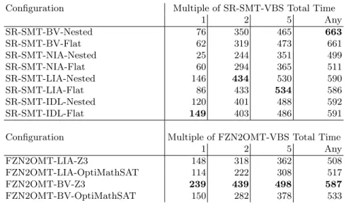
In this section we look at which configurations of SR-SMT are most effective, and how each configuration contributes to the virtual best solver. First we compare Nested to Flat configurations, then we compare the four theories. Also, Table 2 shows how each configuration contributed to the virtual best solver SR-SMT-VBS, and how many additional instances were solved within multiples of 2 and 5 of the VBS time. This gives an overview of how strong the configurations are relative to the VBS.
Configuration Multiple of SR-SMT-VBS Total Time 1 2 5 Any SR-SMT-BV-Nested 76 350 465 663 SR-SMT-BV-Flat 62 319 473 661 SR-SMT-NIA-Nested 25 244 351 499 SR-SMT-NIA-Flat 60 294 365 511 SR-SMT-LIA-Nested 146 434 530 590 SR-SMT-LIA-Flat 86 433 534 586 SR-SMT-IDL-Nested 120 401 488 592 SR-SMT-IDL-Flat 149 403 486 591
Configuration Multiple of FZN2OMT-VBS Total Time
1 2 5 Any
FZN2OMT-LIA-Z3 148 318 362 508
FZN2OMT-LIA-OptiMathSAT 114 222 308 517
FZN2OMT-BV-Z3 239 439 498 587
FZN2OMT-BV-OptiMathSAT 150 282 378 533
Table 2: Number of instances solved by each configuration within multiples of SR-SMT-VBS or FZN2OMT-VBS total time. An instance is counted for
con-figuration X and multiple f if total time for X is withinf× total time for the
VBS. The highest value in each column is highlighted in bold.
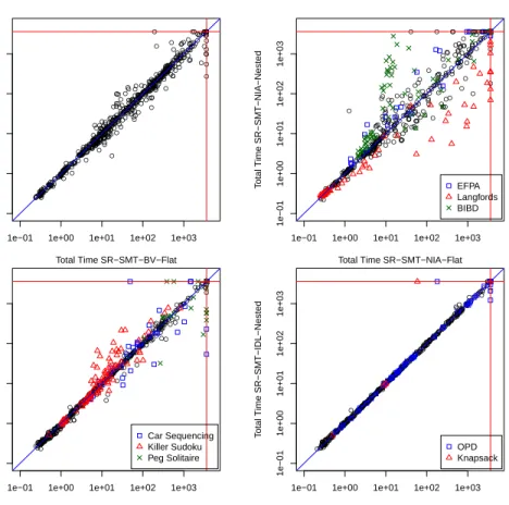
Comparing Nested to Flat Translation Figure 4 compares Nested to Flat configurations for each theory. With the theory of bit-vectors the two configura-tions are remarkably similar. Total number of instances solved and PAR2 score from Table 1 suggest that Nested is slightly better, and Nested is also selected more often in SR-SMT-VBS (Table 2).
With the QF NIA theory, Flat translation performs better overall, solving 12 more instances and with a lower PAR2 score. Some problem classes were solved much better with Flat, such as BIBD (in green). For some instances of EFPA (highlighted in blue), the two encodings are similar, and for others Flat is significantly more efficient. BIBD exhibits increasing gains for Flat as the instances become more difficult. However, Nested is more efficient for Langford’s Problem, solving several instances that Flat cannot.
For the QF LIA theory, we found that almost all problem classes were very similar. There were three exceptions: Killer Sudoku (where the Flat encoding is somewhat better), Car Sequencing, and Peg Solitaire (where the instances are scattered and neither Nested nor Flat seem to have an advantage).
Finally, with QF IDL for almost all problem classes the Nested and Flat encodings were very similar in performance. There are no problem classes where one encoding consistently outperforms the other by a substantial margin.
Comparing Theories The four theories have quite different characteristics and the ideal choice of theory might vary by problem class. To compare the
● ● ● ● ● ● ● ● ● ● ● ● ● ● ●●●● ● ● ● ● ● ● ● ●● ● ● ● ● ● ●● ● ● ● ● ● ● ● ● ● ● ●● ● ● ● ● ● ● ● ● ● ● ● ● ● ●● ● ● ● ● ● ● ● ● ● ●● ● ● ●● ● ● ●●● ● ● ● ● ● ●● ● ● ●●● ● ● ● ● ●●● ● ●● ● ●●●●● ● ●● ● ● ● ●● ● ● ● ● ● ● ● ● ● ● ● ● ● ● ●●●●●●●● ● ●●●●●● ●●●● ● ● ●●● ● ●●● ●● ● ●●●●●●●●●● ● ●●●● ● ● ● ●● ● ● ● ● ● ● ● ● ● ● ● ● ● ● ● ● ● ● ● ● ● ● ● ●● ● ● ● ● ● ● ● ● ● ● ●● ● ● ●● ● ● ● ● ● ● ● ● ● ● ● ●● ● ● ● ● ● ● ● ● ● ● ● ● ● ● ● ● ● ● ● ● ● ● ● ● ● ● ● ● ● ● ●● ● ● ●●●● ● ● ●● ●● ●●● ● ● ● ●●●● ● ● ●●● ●●●●●●●●●●●●●●● ● ● ● ● ● ● ● ● ● ● ● ● ● ● ●● ● ● ● ● ● ● ● ● ● ● ● ● ● ●●● ● ● ● ● ● ● ● ● ●●●●●● ● ● ● ● ● ● ● ● ● ● ● ● ● ● ●●● ● ● ● ● ● ● ● ● ● ● ● ● ● ● ● ● ●● ● ● ● ●● ● ●● ● ● ● ● ● ● ● ● ● ● ● ● ● ● ● ● ● ● ● ● ● ● ● ● ●● ● ● ●●●● ●● ●● ● ● ● ● ● ●●● ●● ● ● ● ● ●● ● ● ●●●● ● ● ● ● ● ● ● ●● ● ● ●●●● ● ● ● ● ● ● ● ● ● ●●●●● ● ●●● ●●● ● ●●●● ● ●● ● ●● ● ● ● ● ● ● ● ●● ● ● ● ● ● ●●● ● ● ● ● ● ● ● ● ● ● ● ● ● ● ● ● ● ● ● ● ● ● ● ● ● ● ● ● ● ● ● ● ● ● ● ● ● ● ●●● ●●● ● ● ● ● ● ● ● ● ● ● ● ● ● ● ● ● ● ● ● ● ● ● ● ● ● ● ● ● ● ● ● ● ●● ● ● ● ● ●● ● ● ● ● ● ● ● ●● ● ● ● ● ● ●● ● ●● ● ●● ● ● ● ● ● ● ● ● ● ● ● ● ● ● ● ● ● ● ● ● ● ● ● ● ● ● ● ● ● ● ● ● ● ● ● ● ● ● ●● ● ● ● ● ● ● ● ● ● ● ● ● ● ● ● ● ● ● ● ● ● ● ● ●● ● ● ● ● ● ● ● ●● ● ● ● ● ● ● ● ● ● ● ● ●● ● ● ● ● ● ● ● ●● ● ● ●● ●●●● ● ● ●●●● ● ● ● ● ● ● ● ● ● ● ● ● ● ● ● ● ●●●●
1e−01 1e+00 1e+01 1e+02 1e+03
1e−01
1e+00
1e+01
1e+02
1e+03
Total Time SR−SMT−BV−Flat
T
otal Time SR−SMT−BV−Nested
● ● ● ● ● ●●● ● ● ● ● ● ● ● ● ● ● ● ● ● ● ● ● ● ● ● ● ● ● ● ● ● ● ● ● ● ● ● ● ● ● ● ● ● ● ● ● ●●●●●● ● ● ● ● ● ● ● ● ● ● ● ● ● ● ● ● ● ● ● ● ● ●●● ●● ●● ●● ●●●●●●●●●●●●●●●●●●●●●●●●●●●●●●●●●●●●●●●●●●●●●●●●●●●●●●●●●●●●●●●●●●●●● ● ● ●● ● ● ●●●● ● ● ● ● ● ● ●● ● ● ● ● ● ● ● ● ● ● ● ● ● ● ● ● ● ●●● ● ● ● ● ● ● ● ● ● ● ● ● ● ● ● ●● ● ● ● ● ● ● ● ● ● ● ● ● ● ● ● ● ● ● ● ● ● ● ● ● ● ● ● ● ● ● ● ● ● ● ● ● ● ●● ● ● ● ● ● ● ● ● ● ● ● ● ● ● ●● ● ● ● ● ● ● ● ● ●●● ● ● ● ● ● ● ● ● ● ● ● ● ● ● ● ● ● ● ● ● ● ● ● ● ● ● ● ● ●● ● ● ● ● ● ● ● ● ● ● ● ● ● ● ● ● ● ● ● ● ● ● ● ● ● ● ● ● ● ● ●● ● ● ● ● ● ● ● ●●●●●● ● ● ●● ● ● ● ● ● ● ● ● ● ● ● ● ● ● ● ● ● ● ● ● ● ● ● ● ● ● ●● ● ● ● ● ● ● ● ● ● ● ● ● ● ● ● ● ● ● ● ● ● ● ● ● ● ● ● ● ● ● ● ● ● ● ● ●● ● ● ● ● ● ● ● ●●●●●●●● ● ● ● ● ● ● ● ● ● ● ● ● ● ● ● ● ● ● ● ● ● ● ● ● ● ● ● ● ● ● ● ● ● ● ●● ● ● ● ● ● ● ● ● ● ● ● ● ● ● ● ● ● ● ● ● ● ● ● ● ● ● ● ● ● ● ● ● ● ● ●●● ● ● ● ● ● ● ● ● ● ● ● ● ● ● ● ● ● ● ● ● ● ● ● ● ● ● ● ● ● ●● ●● ●● ● ● ● ● ● ● ● ● ● ● ● ● ● ●● ● ● ●●● ● ● ● ● ● ● ●● ● ● ● ● ● ● ● ● ● ● ● ● ● ● ● ● ● ● ● ● ● ● ● ● ● ●
1e−01 1e+00 1e+01 1e+02 1e+03
1e−01
1e+00
1e+01
1e+02
1e+03
Total Time SR−SMT−NIA−Flat
T
otal Time SR−SMT−NIA−Nested EFPA Langfords BIBD ● ● ●●● ● ● ●● ● ● ● ●●●● ●● ● ● ● ● ● ● ● ●● ● ● ● ● ● ●● ● ●● ● ● ● ● ● ● ● ●● ● ● ● ● ● ● ● ● ● ● ● ● ● ● ● ●● ● ● ● ● ● ● ● ●● ●● ●● ● ●● ● ●●●● ● ● ●●● ● ● ● ● ● ● ● ● ● ● ● ● ● ● ●●●●● ● ●● ● ● ● ●● ● ● ● ● ● ● ● ● ● ● ● ● ● ● ● ● ● ● ●●●● ● ●● ● ● ● ● ● ● ● ● ● ● ● ● ● ● ● ● ● ● ● ● ● ● ● ● ● ● ● ●● ●● ● ● ● ● ● ● ● ● ● ● ● ● ● ● ● ● ● ●●● ● ● ● ● ●●●● ● ● ● ●● ●●●● ● ● ● ●●●●●●●●●●●●●●●●●● ●●●●●● ● ● ● ● ● ● ● ● ● ●●●●●●● ● ● ● ● ● ● ●●●●●●● ●● ● ● ● ● ● ● ●●● ●●●● ●● ● ● ● ● ●●●●● ●●● ●●● ● ● ●●●●●●● ● ●●●● ●●●● ●● ● ● ● ● ● ● ● ● ● ● ● ● ● ● ● ● ●● ● ● ● ●●● ● ● ● ●● ● ● ● ● ● ● ● ● ● ● ● ● ● ● ● ● ● ● ● ● ● ● ● ●● ● ● ● ● ● ● ● ●● ●●●● ● ● ● ● ● ● ● ● ● ● ● ● ● ● ● ● ● ● ● ● ● ● ● ● ● ● ● ● ● ● ● ● ● ● ● ● ● ● ● ● ● ● ● ● ● ● ● ●● ● ● ● ● ● ● ● ● ●● ●● ●● ● ● ● ● ● ●● ●● ●● ● ● ● ● ● ● ● ● ● ● ● ● ● ● ● ● ● ● ● ● ● ● ● ● ● ● ● ● ● ● ● ● ● ● ● ● ●● ●● ●●●●● ● ● ● ● ●● ● ● ● ● ● ● ●●● ● ● ● ●● ● ● ● ● ● ● ● ● ● ● ● ● ● ● ● ● ● ● ● ● ● ● ● ● ● ● ● ● ●
1e−01 1e+00 1e+01 1e+02 1e+03
1e−01
1e+00
1e+01
1e+02
1e+03
Total Time SR−SMT−LIA−Flat
T
otal Time SR−SMT−LIA−Nested
Car Sequencing Killer Sudoku Peg Solitaire ● ● ● ● ● ● ● ● ● ● ● ● ● ● ● ● ● ● ● ● ● ● ● ● ● ● ● ● ● ● ● ● ● ● ● ●● ● ● ● ● ● ● ● ●● ● ● ●● ● ● ● ● ● ● ● ● ● ● ● ●● ● ● ● ● ● ● ● ●● ● ● ●● ● ● ● ● ● ●● ● ● ●●●● ● ● ● ● ● ● ● ● ● ● ● ● ●● ●●●●●● ●● ● ● ● ● ● ● ● ● ● ● ● ● ● ● ● ● ● ● ● ● ● ●● ●●●● ● ● ● ● ●●● ●●●● ● ● ●● ● ● ● ● ●●●● ● ●● ● ● ● ● ● ● ● ● ● ● ● ● ● ● ● ● ●● ● ● ● ●● ● ● ● ● ● ● ●● ● ● ● ● ● ● ● ● ● ● ● ● ● ● ● ● ● ● ● ● ● ● ●● ●● ● ● ● ●● ● ● ● ● ● ● ● ● ● ● ● ● ● ● ● ● ● ● ● ● ● ● ● ● ●● ● ● ● ● ● ● ● ● ● ● ● ● ● ●●● ● ● ● ● ● ● ● ● ●● ●● ● ●●●● ●●●●● ● ● ● ●●●●●●●●●●●●●●●●● ● ● ●● ● ● ● ● ● ● ● ● ● ● ● ● ● ● ● ● ● ● ● ● ● ● ● ● ● ●●●● ● ● ● ● ● ● ● ●● ● ● ● ● ● ● ● ● ● ● ● ● ● ● ● ● ● ● ● ● ● ● ● ● ● ● ● ● ● ● ● ● ● ● ● ● ● ● ● ● ● ● ●● ● ● ● ● ● ● ● ● ● ● ● ● ● ● ● ● ● ●● ● ● ●● ● ●●● ●●●● ● ● ● ● ● ● ●● ●● ●●●● ● ●● ● ● ●●●●● ●●●● ●●● ● ● ● ● ●●●● ●●● ●●●●● ●●●●●●● ● ● ●●●●● ● ●●●● ● ● ● ● ● ● ● ● ● ● ● ● ● ● ● ● ● ● ● ●●● ●● ● ● ● ● ● ● ● ● ● ● ● ● ● ● ● ● ● ● ● ● ● ● ● ● ● ● ● ●● ● ● ● ● ● ● ●● ● ●●●●● ● ●● ● ● ● ● ● ● ● ● ● ● ● ● ● ● ●● ● ● ● ● ●● ● ● ● ● ● ● ● ●● ● ● ● ● ● ● ● ● ● ● ● ●● ● ● ● ● ● ● ●●● ● ● ● ● ●● ●● ● ● ●● ● ●● ● ● ● ● ● ● ●● ● ● ● ● ● ● ● ●● ● ●
1e−01 1e+00 1e+01 1e+02 1e+03
1e−01
1e+00
1e+01
1e+02
1e+03
Total Time SR−SMT−IDL−Flat
T
otal Time SR−SMT−IDL−Nested
OPD Knapsack
Fig. 4: Nested vs Flat translation for each theory, total time.
four theories, for each one we take the better configuration (of Nested or Flat), so we compare SR-SMT-BV-Nested, SR-SMT-NIA-Flat, SR-SMT-LIA-Nested, and SR-SMT-IDL-Nested. BV is the strongest theory in terms of instances solved within 1 hour and PAR2 score, therefore we use BV as the gold standard and compare the other theories to it.
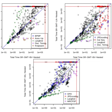
Figure 5 (top left) plots NIA-Flat against BV-Nested. Many instances time out with NIA-Flat, for example the majority of Aces-Up (in red), and all in-stances of the block party metacube problem (BPMP, in blue). Langford’s Prob-lem is an example where the two theories are correlated, but BV is more efficient on the bulk of the instances. In contrast, Discrete Tomography is solved more efficiently by NIA-Flat. In this case, Z3 internal heuristics decide to convert the QF NIA formula into a QF BV formula before solving, and this is more efficient than Boolector directly applied to the BV-Nested formula. Also, both NIA en-codings contribute a relatively small number of instances to the VBS (Table 2).
LIA-Nested is plotted against BV-Nested in Figure 5 (top right). Langford’s Problem and Discrete Tomography are examples where LIA-Nested performs substantially better than BV-Nested. The constraints in these problems are well suited to the QF LIA theory (in particular Discrete Tomography, where all con-straints are linear). Car Sequencing is split, some instances are solved more quickly by LIA-Nested while others time out. All instances of JPEncoding are solved more efficiently by LIA-Nested. Overall BV-Nested has a substantial edge: it is able to solve 73 more instances and its PAR2 score is much lower.
Finally, we compare IDL-Nested to BV-Nested in Figure 5 (lower). MR-CPSP (the multi-mode resource-constrained project scheduling problem) has precedence constraints that are naturally expressed in IDL. The most difficult instances of MRCPSP are solved more efficiently by IDL-Nested. Langford’s Problem is also solved more efficiently by IDL-Nested. OPD is mixed but shows large speed-ups for BV for some of the most difficult instances. Many instances time out for IDL-Nested and are solved with BV-Nested, e.g. all instances of the JPEncoding problem. In total, 71 more instances are solved by BV-Nested.
In summary, we have seen several cases where NIA, LIA, or IDL performs well on a problem class and in these cases the problem class has constraints that are naturally expressed in the theory. For example, Discrete Tomography (with linear constraints) is solved very well by LIA-Nested (and also by NIA-Flat, where the solver converts it into a QF BV formula). In contrast, BV seems the most robust. It performs well on a wide range of problem classes and in each comparison solves many instances that the other configuration did not.
4.4 Analysis of FZN2OMT
Table 2 gives an overview of how each configuration of FZN2OMT contributes to the virtual best solver, FZN2OMT-VBS. The BV encoding with Z3 is clearly the strongest combination on these benchmarks, contributing the most instances to the VBS and also solving the most within 1 hour. Z3 was more effective than OptiMathSAT on the BV formulas, however the picture is not so simple with LIA. OptiMathSAT seems to be stronger overall on LIA formulas, solving more instances within 1 hour, however Z3 contributes more instances to the VBS.
4.5 Comparison to SAT
As described in Section 3, all SR-SMT encodings are built on the default SAT
encoding of Savile Row, so comparison between SR-SMT and SAT is
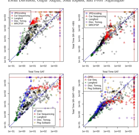
partic-ularly relevant. We use CaDiCaL as the SAT solver and use the default options for the SAT backend. Figure 6 (top left) plots SAT against the strongest SMT configuration, SR-SMT-BV-Nested. The two are quite similar in overall perfor-mance, with similar PAR2 scores. SAT solves 8 more of the benchmark instances than SR-SMT-BV-Nested (Table 1). Some problem classes are solved more ef-ficiently by SAT, such as Discrete Tomography, Langford, and MRCPSP. In contrast, SR-SMT-BV-Nested is able to solve 6 out of 10 instances of JPEn-coding whereas SAT solves none. Car Sequencing is mixed but the majority of
● ● ● ● ● ● ● ● ● ● ● ● ● ● ● ● ● ● ● ●●●● ● ● ● ● ● ● ● ● ● ● ●● ● ● ●● ● ● ● ● ● ● ● ● ● ●● ● ● ● ● ● ● ● ● ● ●● ● ● ● ● ● ● ● ● ● ● ● ● ● ● ● ● ● ● ●●●● ● ● ● ● ● ● ● ● ● ● ● ● ●● ● ● ● ● ● ● ● ● ● ● ● ● ● ● ●●●● ●●●● ● ● ● ●● ●●●●●● ● ● ● ● ●●●●●●●●●● ●●●●●●●● ●●●●●● ●●●●●●●●●●●● ●●●●●●●●●●●● ● ● ● ● ● ● ● ● ● ● ● ● ● ● ● ● ● ● ● ● ● ● ● ● ● ● ●● ● ● ● ● ● ●●●● ● ● ● ● ● ● ● ● ● ● ● ● ● ● ● ●● ● ● ● ● ● ● ● ● ● ● ● ● ● ● ● ● ● ●●● ● ● ●●● ●●●●●●●●●●●●●●● ● ● ●● ● ● ● ● ● ● ● ● ● ● ●● ● ● ● ● ● ● ●● ● ● ● ● ● ●●● ●● ● ● ● ● ● ● ●● ● ● ● ● ● ● ● ● ● ● ● ● ● ● ● ● ● ● ● ● ● ● ● ● ● ● ● ● ● ● ● ● ● ● ● ● ● ●● ● ● ● ● ● ●● ● ● ●● ● ● ● ● ● ● ● ● ● ● ● ● ● ● ● ● ●● ●●● ●● ● ● ● ● ● ● ● ● ● ●● ●● ●●● ● ● ● ● ● ●● ● ● ● ● ● ● ● ● ● ● ● ● ● ● ● ● ● ● ● ● ● ● ● ●●●● ● ● ● ● ● ● ● ● ● ● ● ● ●●● ● ●● ● ● ● ● ● ● ● ● ● ● ● ● ● ● ● ● ● ● ● ● ● ● ● ● ● ● ● ● ● ● ● ● ● ● ● ● ● ● ● ● ● ● ● ● ● ● ● ● ● ● ●● ● ● ●● ● ●● ●● ●● ● ● ●● ● ● ● ● ● ● ● ● ● ● ● ● ● ● ● ● ● ● ● ● ● ● ● ● ● ● ● ● ● ● ● ● ● ● ● ● ● ● ● ● ● ● ● ● ●● ●●● ● ● ● ●● ● ● ● ● ● ● ● ● ● ● ● ● ● ●● ● ● ● ●●●● ● ● ● ● ● ● ● ● ● ● ● ● ● ● ● ● ● ●●● ● ●● ● ● ● ● ● ● ● ● ● ● ● ●● ● ● ● ● ● ● ● ● ● ● ● ● ●
1e−01 1e+00 1e+01 1e+02 1e+03
1e−01
1e+00
1e+01
1e+02
1e+03
Total Time SR−SMT−BV−Nested
T
otal Time SR−SMT−NIA−Flat
BPMP Aces−Up Langford Disc. Tomog. Knapsack ●● ● ● ●●●● ● ● ● ● ● ● ● ● ● ● ● ● ● ● ●● ● ● ● ● ● ●● ● ● ● ● ● ● ● ● ● ● ● ● ● ● ● ● ● ● ● ● ● ● ● ● ● ● ● ● ● ●● ● ● ●● ● ● ● ●● ● ●● ● ● ●● ● ● ● ● ● ● ● ● ● ● ● ● ● ● ● ● ●●●● ● ● ● ● ● ● ● ● ● ● ● ● ●● ● ● ● ● ● ● ● ● ● ● ● ● ● ● ● ● ● ● ● ● ● ● ● ● ● ● ● ● ● ● ● ● ● ● ● ● ● ● ● ● ● ● ● ● ● ● ● ● ● ● ● ● ● ● ● ●●● ● ●● ● ● ● ● ● ● ● ● ● ● ●● ● ● ●●● ● ● ● ●●● ●●●●●●●●●●●●●●● ● ● ● ● ● ● ● ● ● ● ● ● ● ● ●● ● ● ● ● ● ● ● ● ● ● ● ● ● ● ● ● ● ● ● ● ● ● ● ● ● ● ● ● ● ● ● ● ● ● ● ● ● ● ● ● ● ● ● ● ● ● ● ● ● ● ● ● ● ● ● ● ● ● ● ● ● ● ● ● ● ● ● ● ● ● ● ● ● ● ● ●● ● ● ● ● ● ● ● ● ● ●●● ● ● ● ● ● ● ● ● ● ●●● ● ●● ●● ● ● ● ● ● ● ● ● ● ● ● ● ●●● ● ● ● ● ● ●● ● ●● ● ● ● ● ● ● ● ● ● ● ● ● ● ● ● ● ● ● ● ● ●●●● ● ● ● ● ● ● ● ● ● ● ● ● ●●●● ●● ● ● ● ● ● ● ● ● ● ● ● ● ● ● ● ● ● ● ● ● ● ● ● ● ● ● ● ● ● ● ● ● ● ● ● ● ● ● ● ● ● ● ● ● ● ● ● ●● ● ● ● ● ● ●● ● ●● ●● ● ● ● ● ● ● ● ●● ●● ●● ● ● ● ● ● ● ● ● ● ● ● ● ● ● ● ● ● ● ● ● ● ● ● ● ● ● ● ● ● ●● ● ● ● ● ● ● ● ● ● ● ●● ● ● ● ● ● ● ● ● ● ●●● ● ● ● ● ● ●● ● ● ● ●●●● ● ● ● ● ●● ● ● ● ● ● ● ● ● ● ● ● ●● ● ● ● ● ● ● ● ● ●● ● ● ● ● ● ● ● ● ● ● ● ● ● ● ● ● ●●●●
1e−01 1e+00 1e+01 1e+02 1e+03
1e−01
1e+00
1e+01
1e+02
1e+03
Total Time SR−SMT−BV−Nested
T
otal Time SR−SMT−LIA−Nested
JPEncoding Car Seq. Langford Disc. Tomog. ●● ● ● ●●●● ● ● ● ● ● ● ● ● ● ● ● ● ● ● ● ● ● ● ● ● ● ●● ● ● ● ●● ● ● ●● ● ● ● ● ● ● ● ● ● ● ● ● ● ● ● ● ● ● ● ● ●● ● ● ●● ● ● ● ● ● ● ● ● ● ● ●● ● ● ● ● ● ● ● ● ● ●● ● ● ● ● ● ●●●● ● ● ● ● ● ● ● ● ● ● ● ● ●● ● ● ● ● ● ● ● ● ● ● ● ● ●● ●● ● ● ● ● ● ● ● ●● ●● ● ● ●● ● ● ● ● ●● ●● ● ●● ● ● ● ● ● ● ● ● ● ● ● ● ● ● ● ● ●● ● ● ● ●● ● ● ● ● ● ● ●● ● ● ● ● ● ● ● ● ● ● ●● ● ● ● ● ● ● ● ● ● ● ●● ● ● ●● ● ● ● ● ● ● ● ● ● ● ● ● ● ● ● ● ● ● ● ● ● ● ● ● ● ● ● ● ● ● ● ● ● ● ● ● ● ● ● ● ● ● ● ●● ●● ● ● ● ● ● ● ● ● ● ● ● ● ●●● ● ●●●● ● ● ● ●● ●●●●●●●●●●●●●●● ● ● ●● ● ● ● ● ● ● ● ● ● ● ●● ● ● ● ● ● ● ● ● ● ● ● ● ● ●●● ● ● ● ● ● ● ● ● ●● ● ● ● ● ● ● ● ● ● ● ● ● ● ● ● ● ● ● ● ● ● ● ● ● ● ● ● ● ● ● ● ● ● ● ● ● ● ● ● ● ● ● ● ● ● ● ● ● ● ● ● ● ● ● ● ● ● ● ● ● ● ● ● ● ● ● ● ● ● ● ● ● ●●● ● ● ●●● ● ● ● ● ● ● ● ● ● ● ● ● ●●● ● ● ● ● ● ●● ● ● ● ● ● ● ● ● ● ● ● ● ● ● ● ● ● ● ● ● ● ● ● ●● ● ● ●● ● ● ● ● ● ● ● ● ● ● ● ● ● ● ● ● ● ● ● ● ● ● ● ● ● ● ● ● ● ●● ● ● ● ● ● ● ● ● ● ● ● ●● ● ● ● ● ● ● ● ● ● ● ● ●● ● ●●● ● ● ●● ● ● ● ● ● ● ● ● ● ●● ● ● ● ● ● ● ● ●● ● ●
1e−01 1e+00 1e+01 1e+02 1e+03
1e−01
1e+00
1e+01
1e+02
1e+03
Total Time SR−SMT−BV−Nested
T
otal Time SR−SMT−IDL−Nested OPD JPEncoding Langford MRCPSP
Fig. 5: Comparison of the four theories using the better configuration for each one (of Nested or Flat).
instances are solved more efficiently by SAT. 644 instances are solved by both SAT and BV-Nested, and of those the majority (510) are solved faster by SAT. Figure 6 (top right) plots SAT against SR-SMT-VBS. The VBS solves a further 22 instances compared to BV-Nested (14 more than SAT), and improves on various problem classes including Langford, Discrete Tomography, MRCPSP, and Car Sequencing. For the 657 instances that are solved by both the VBS and SAT, the majority (337) are solved more efficiently by SAT, however the VBS has a better PAR2 score (by over 100 seconds). The VBS is of course a theoretical solver, but these results show the value of selecting an appropriate theory for a given instance. As part of our future work we intend to investigate algorithm selection methods to construct a portfolio of the 8 SR-SMT configurations.
We found that the QF IDL encodings were the largest, with a median clause ratio of 104.5% for both IDL-Nested and IDL-Flat compared to SAT. The QF LIA encodings were more compact, with median clause ratios of 15.7% for