Fast Variational Bayesian Inference for Non-Conjugate Matrix
Factorization Models
Matthias Seeger
Probabilistic Machine Learning Laboratory
Ecole Polytechnique F´ed´erale de Lausanne
INR 112, Station 14, CH-1015 Lausanne
[email protected]
Guillaume Bouchard
Xerox Research Centre Europe
6, Chemin de Maupertuis, 38240 Meylan, France
[email protected]
February 15, 2012
Abstract
Probabilistic matrix factorization methods aim to extract meaningful correlation structure from an incomplete data matrix by postulating low rank constraints. Recently, variational Bayesian (VB) inference techniques have successfully been ap-plied to such large scale bilinear models. How-ever, current algorithms are of the alternate up-dating or stochastic gradient descent type, slow to converge and prone to getting stuck in shal-low local minima. While for MAP or maximum margin estimation, singular value shrinkage al-gorithms have been proposed which can far out-perform alternate updating, this methodological avenue remains unexplored for Bayesian tech-niques. In this paper, we show how to combine a recent singular value shrinkage characterization of fully observed spherical Gaussian VB matrix factorization with local variational bounding in order to obtain efficient VB inference for general MF models with non-conjugate likelihood poten-tials. In particular, we show how to handle Pois-son and Bernoulli potentials, far more suited for most MF applications than Gaussian likelihoods. Our algorithm can be run even for very large models and is easily implemented inMatlab. It exhibits better prediction performance than MAP estimation on several real-world datasets.
Appearing in Proceedings of the15th
International Conference on Artificial Intelligence and Statistics (AISTATS) 2012, La Palma, Canary Islands. Volume XX of JMLR: W&CP XX. Copyright 2012 by the authors.
1
Introduction
Matrix factorization (MF) models are widely used in ma-chine learning and applications, for reduced rank regres-sion [13], sparse principal components analysis [12], par-tial least squares [14], multi-task learning [3], latent se-mantic indexing [4], or collaborative filtering [7]. Ma-chine learning approaches include maximum margin MF [17], maximum a posteriori (MAP) estimation [17, 15] and, more recently, variational Bayesian inference [11, 8, 12, 9]. Whether maximum margin, MAP or variational Bayes, methods for learning MF models from data roughly fall into two different classes. First, alternate minimization or stochastic gradient descent methods are based on efficient and simple updates, which directly exploit both the spar-sity in the likelihood and the bilinear model structure. For example, alternate minimization solves for one matrix at a time, keeping the other fixed, then iterates this process in a round-robin fashion. In VB, the posterior over matrices is assumed to factorize, which at least in conjugate like-lihood cases leads to simple updates of posterior factors. These are iterated over in the same fashion. While easily implemented and scaled up to large problems, these tech-niques tend to converge exceedingly slowly and are prone to getting stuck in poor local minima, necessitating mul-tiple restarts and additional heuristics. The second class of algorithms is based on recent fundamental results which establishanalytical solutionsfor certain basic MF models [19, 17, 2, 9], essentially by computing a singular value de-composition (SVD) and shrinking or thresholding the sin-gular values. Can these exact characterizations be used in order to learn generalMF models, as subroutines of iter-ative algorithms, much like Newton-Raphson optimization 1
is based on quadratic minimization? If so, we should end up with algorithms which are much faster to converge and behave more robustly than methods based on simple gradi-ent descgradi-ent or alternate updating. Moreover, due to its vast impact on diverse applications, very efficient, highly par-allelizable code for approximate SVD is available to drive MF learning algorithms. This idea has been realized both for maximum margin and MAP estimation [17, 20, 18], while all previous variational Bayesian algorithms for gen-eral models belong to the first class [11, 8].
Our main contribution in this paper is a novel SVD-based algorithm for variational Bayesian inference in matrix fac-torization models with general likelihoods. The main prim-itive driving our method is a recent SVD shrinkage char-acterization of VB matrix factorization for complete data spherical Gaussian likelihood [9]. We show how to solve VB inference problems for realistic MF models with highly incomplete Poisson or Bernoulli likelihoods at the expense of a few calls to approximate SVD code. Our method can be formulated entirely in terms of sparse or low rank ma-trices, and it is easily scaled up to very large problems. Its computational cost per iteration is equivalent to SVD-based algorithms for MF MAP estimation [20, 18]. The struc-ture of this paper is as follows. We discuss related work in Section 2. In Section 3, we introduce the variational Bayesian matrix factorization setup and review an analyti-cally solvable special case [9]. Our algorithm is derived in Section 4. We comment on non-conjugate likelihood po-tentials in Section 4.1 and describe our large-scale imple-mentation in Section 4.2. We present experimental results on a range of real-world datasets in Section 5, and close with conclusions in Section 6.
2
Related Work
Matrix factorization (MF) models are core components of collaborative filtering or recommender systems and have attracted a large amount of research to date. We restrict our focus to probabilistic approaches. Maximum a poste-riori (MAP) estimation for MF models or closely related “maximum margin” variants was pioneered in [17], where the link to SVD with shrinkage on the spectrum was ob-served. Previously, an analytical solution based on eigen-decomposition was established for probabilistic principal components analysis in [19]. The MAP interpretation of the method of [17], as well as the link to nuclear-norm reg-ularization, was made explicit in [15].
More recently, variational Bayesian inference methods have been proposed [11, 8], where factors are integrated out approximately rather than estimated. While easy to im-plement and scalable to large problems, previous VBMF algorithms are alternate updating or stochastic gradient de-scent variants, which converge slowly and are prone to get-ting stuck in poor local optima. A key result for VBMF
is the global analytical solution for the Gaussian complete likelihood case established in [9], of pivotal importance for our work here.
3
Variational Bayesian Matrix Factorization
Suppose our goal is to predict missing entries in am×n matrixY from observationsyij,(ij) ∈ O. For example, themrows may index users of an e-commerce website, the ncolumns items on sale, and the goal is to make recom-mendations. If|O| mn, it is essential to share statistical strength by learning latent correlations between the groups, which in bilinear matrix factorization models are repre-sented via a jointr-dimensional space, r min{n, m}. We specify latent factors U ∈ Rm×r, V ∈Rn×r, and
setX = UVT ∈
Rm×n. Here,U = [uk],V = [vk],
k = 1, . . . , r, whereuk ∈ Rm,vk ∈Rn are the columns
which span the latent low-dimensional representation. For the likelihood, we assume thatP(Y|U,V) =P(Y|X), whereP(Y|X)factorizes w.r.t. matrix entries:
P(Y|X) = Y
(ij)∈O
P(yij|xij), xij =
r
X
k=1
uikvjk.
In this paper, we are interested in general likelihood poten-tialsP(yij|xij)which do not admit conjugacy properties. For the prior, we assume the following factorized form:
P(U,V) =
r
Y
k=1
P(uk)P(vk).
Bayesian inference is generally intractable in matrix factor-ization models, even in the case of conjugate Gaussian like-lihood potentials. The problem arises from product cou-plings uikvjk in the likelihood, which can give rise to a complex posterior distribution P(U,V|Y). In the varia-tional Bayesian(VB) approach, we approximate the poste-rior with a distributionQ(U,V)from a tractable class, by minimizing F = EQ(U,V) log Q(U,V) P(Y|U,V)P(U,V) = D[Q(U,V)kP(U,V|Y)]−logP(Y). (1)
We focus on variational distributions of the factorized form Q(U,V) =
r
Y
k=1
Q(uk)Q(vk). (2)
In other words,Q(U,V)admits the same factorization be-tween pairs of columns of[U V]as the prior.
Even with these simplifying assumptions, the minimiza-tion of (1) is not a simple problem. The most frequently chosen approach is to updateQ(U)andQ(V)in turn [8].
However, such alternate updating algorithm are notoriously prone to getting stuck in poor local minima. Our main con-tribution is an algorithm which fares much better in gen-eral, by exploiting recent results about a special case of (1) which can be solved analytically.
3.1 Fully Gaussian Complete Likelihood: G-VBMF Maybe the simplest instance of VBMF is the spherical Gaussian complete likelihood case, called G-VBMF in the sequel. Here, all entries of Y ∈ Rm×n are ob-served (O={1, . . . , m} × {1, . . . , n}), andP(yij|xij) =
N(yij|xij, σ2)is Gaussian. The noise varianceσ2has to
be the same for all likelihood potentials. Moreover, the pri-ors are Gaussian as well:
P(U) =Y k N(uk|0, c2u,kI), P(V) = Y k N(vk|0, c2v,kI).
It is straightforward to apply alternating minimization to (1) in this case [8], yet the problem remains non-convex. Importantly, Nakajimaet.al.[9] showed that its global min-imum points, unique up to obvious orthonormal symme-tries, can be solved for analytically. Ifλk,u˜k,v˜kare ther largest singular values, left and right singular vectors ofY, so thatUΛ˜ V˜T is closest toY in Frobenius1norm among all rankrmatrices, then for a global minimum pointQ∗of (1):
EQ∗UVT= EQ∗[U]EQ∗[V]T = ˜U(diagγ) ˜VT,
where the elements γk of γ are closed form functions depending on λk, σ2, c2
u,k, c
2
v,k, m and n. Essentially,
EQ∗[UVT]is obtained fromUΛ˜ V˜T by leaving the
matri-ces in place, but shrinkingλk →γkin a specific way [9]. This characterization allows us to circumvent error-prone alternating minimization entirely.
In practice, the G-VBMF setup is severely restricted. It requires a complete likelihood function with potentials on each entry ofY, which have to be Gaussian and must share the same variance. These restrictions do not make much sense for our recommender system example, a prototypi-cal application of matrix factorization models. The likeli-hood is incomplete by default. Moreover, observed entries ofY are binary or natural numbers, which are poorly rep-resented by a spherical Gaussian likelihood. In the next section, we show how to combine the G-VMBF result with variational bounding techniques in order to overcome these restrictions.
4
An Algorithm for General Potentials
Our aim is to solve the VBMF problem (1) in the general case described in Section 3, yet to make use of the ana-lytical G-VBMF solution of Section 3.1 to drive our al-gorithm. Technically speaking, we have to approximate1
The Frobenius norm is defined askAk2= (trATA)1/2.
the likelihood P(Y|X)by a Gaussian with spherical co-variance (all co-variances equal). While this is certainly a bad one-off approximation, we will introduce variational parameters which determine the (pseudo-)observations Y in G-VBMF, then iteratively improve the fit to the poste-rior distribution. For simplicity, we assume that the pposte-rior P(U,V)already has the form required by G-VBMF, so we only have to deal with the likelihood. An extension to more general Gaussian or non-Gaussian priors can be obtained in much the same way.
We can writeminQFfrom (1) as
min Q(U,V) EQ −logP(Y|UVT) + D[QkP], where D[QkP] = D[Q(U,V)kP(U,V)]. Introducing X=UVT = [xij], we can write
−logP(Y|UVT) =X
i,j
fij(xij), xij=
r
X
k=1
uikvjk,
where fij(xij) = −logP(yij|xij) for (ij) ∈ O, fij(xij) = 0otherwise. We require that the fij(xij)are twice differentiable and
fij00(xij)≤κ ∀xij∀i, j.
We demonstrate below how to chooseκfor Bernoulli and Poisson likelihoods. Now, by Taylor’s theorem:
fij(xij)≤ κ
2(xij−ξij)
2+f0(ξij)(xij−ξij) +fij(ξij).
| {z }
=:qij(xij;ξij)
Plugging these tight bounds into the criterion and inter-changingEQ[. . .]andmin[ξij](which weakens the bound),
we obtain our final variational optimization problem:
min
Q(U,V),[ξij]
X
ij
EQ[qij(xij;ξij)] + D[QkP].
Our algorithm alternates between updates of [ξij] and of Q(U,V). For the former, the criterion decouples addi-tively, so each ξij can be updated independently. Since qij is a quadratic, we have that EQ[qij(xij;ξij)] = qij(EQ[xij];ξij) +Cij, whereCij does not depend onξij. Now,
qij(EQ[xij];ξij)≥fij(EQ[xij]) =qij(EQ[xij]; EQ[xij]), so that the update isξij ←EQ[xij], or compactly
[ξij]←E[U]E[V]T. For the update ofQ(U)Q(V), note that
qij(xij;ξij)=. κ
2(xij−(ξij−f
0(ξij)/κ))2
.
where “=.” denotes equality up to a constant independent ofxij. Therefore, for fixed[ξij], the update ofQ(U)Q(V)
is equivalent to G-VBMF with pseudo-dataY˜= [˜yij]and varianceσ2= 1/κ. We can solve forE[UVT]analytically, as noted in Section 3.1. Our algorithm iterates between up-dates of[ξij], ofY, and calls of G-VBMF. It is summarized˜ in Algorithm 1.
Algorithm 1General VBMF Algorithm
E[U]←0,E[V]←0. whilenot convergeddo
Update[ξij]←E[U]E[V]T.
UpdateE[U]E[V]T by G-VBMF analytical solution, based on pseudo-dataY˜= [ξij−f0(ξij)/κ].
end while
4.1 Bounds for Likelihood Potentials
In this section, we establish quadratic upper bounds on
−logP(y|x) both for binary classification (Bernoulli) and Poisson likelihood potentials. In both cases, x 7→ −logP(y|x)is a convex function (the potentials are log-concave). While the posterior distribution P(U,V|Y)is complicated due to the product couplingUVT in the like-lihood, log-concave potentials at least do not add additional complexities. Moreover, sincef00
ij(xij)≥0, our quadratic bounds are tighter in this case. Essentially,fij(xij)is sand-wiched between the upper boundqij(xij;ξij)and the linear lower boundf0(ξij)(xij−ξij) +fij(ξij).
If reponses are binary,y∈ {0,1}, a Bernoulli likelihood is appropriate:
P(y|x) = e
yx
1 +ex, f(x) = log (1 +e
x)−yx.
Clearly, f(x)is convex. Moreover, f0(x) = π(x)−y, π(x) = 1/(1 +e−x) andf00(x) = π(x)π(−x) ≤ 1/4.
For Bernoulli likelihood potentials, we can use a quadratic bound withκ= 1/4. Moreover, we update
˜
yij =ξij−fij0 (ξij)/κ=ξij−4(π(ξij)−yij). Note that this bound tends to be looser than Jaakkola’s bound [5] (see [6] for numerical experiments comparing the two). The latter allows for the curvature termκto de-pend onξij as well. While Jaakkola’s bound still leads to Gaussian updates forQ(U)andQ(V), its heteroscedastic-ity would not allow for the reduction to G-VBMF, since the latter calls for a homoscedastic likelihood.
Ify ∈ N = {0,1, . . .}, we can use a Poisson likelihood
with rate functionλ(x)>0:
P(y|x)∝λ(x)ye−λ(x), f(x) =λ(x)−ylogλ(x). (3) It has been shown in [10] that P(y|x) is log-concave (x 7→ −logP(y|x)is convex) ifλ(x)is both convex and
log-concave. A simple choice satisfying this property is λ(x) = ex. The problem with this rate function is its exponential growth for large x, which implies non-robust behaviour in the presence of outliers. Moreover,ex does not have bounded curvature, so our reduction to G-VBMF would not work.
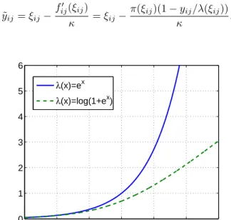
In order to remedy these problems, we propose a novel link function not previously used in this context, λ(x) = log(1 +ex). It is well known thatλ(x)is convex, and we prove log-concavity at the end of this section. It shares with exthe exponential decay asx→ −∞, yet grows only lin-early (with slope approaching1) for largex(see Figure 1). Finally, we need to boundf00(x). First,λ00(x)≤ 1/4, as seen above. Second, it is confirmed by inspection that the second derivative of−log log(1 +ex)is upper bounded by
0.17, so that
fij00(xij)≤κ= 1/4 + 0.17ymax, ymax= max ij yij. Not surprisingly, our bound degrades with the presence of entries with largeyij. In our experiments, we follow com-mon practice and clip overly large counts. We update
˜ yij =ξij− fij0 (ξij) κ =ξij− π(ξij)(1−yij/λ(ξij)) κ . −30 −2 −1 0 1 2 3 1 2 3 4 5 6 λ(x)=ex λ(x)=log(1+ex)
Figure 1: Rate functionsλ(x)for Poisson potentials used in this paper.
Finally, we establish the log-concavity ofλ(x) = log(1 +
ex). First, λ0(x) = π(x) = (1 +e−x)−1, π0(x) = π(x)π(−x) = π(x)2e−x. If g(x) = logλ(x), then g0(x) =π(x)/λ(x), g00(x) = 1 λ(x) π0(x)−π(x) 2 λ(x) = π(x) 2 λ(x) e−x− 1 λ(x) .
Now,log(1 +x)≤x, so that−1/λ(x)≤ −e−x, therefore g00(x)≤0, so thatg(x)is concave.
0 10 20 30 40 50 0.49 0.5 0.51 0.52 0.53 0.54 0.55 0.56 number of iterations log−probability/#data Train K=1 Test K=1 Train K=2 Test K=2 Train K=3 Test K=3 0 10 20 30 40 50 −0.1 0 0.1 0.2 0.3 0.4 0.5 0.6 number of iterations log−probability/#data Train K=1 Test K=1 Train K=2 Test K=2 Train K=3 Test K=3
Binary potentials Poisson potentials
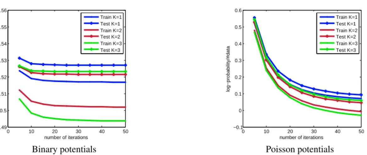
Figure 2: Learning curves for binary and Poisson potential on the Bus Stops dataset for several values of the latent feature dimension. The vertical axis is the normalised log-likelihood computed on train/test data.
4.2 Large-Scale Implementation
Most real-world applications of MF models feature very largemandnalong with sparse observations:|O| mn. Bothmandncan be in the tens or hundreds of thousands, and |O|can be many millions. Viewed in this light, the analytical solution of G-VBMF in terms of an SVD of a m ×n matrix (Section 3.1) seems much less attractive. Storing or even building a dense matrix of this size is far beyond tractability, let alone performing an SVD at the cost ofO(max{m, n}min{m, n}2). For reasons such as these,
SVD-based algorithms are not used much in machine learn-ing, where simpler alternate updating or stochastic gradient descent algorithms are preferred. In this section, we show that our VBMF algorithm, while based on SVD, can nev-ertheless be run at very large scales, using code which is publicly available and in fact part ofMatlab. Our observa-tions, which are related to what is proposed in [20], should be useful beyond the VBMF algorithm of interest here. Recall the VBMF updates from Algorithm 1. We will show that beyondE[U]∈Rm×randE[V]∈Rn×r, only sparse
matrices with|O|non-zeros have to be maintained. First,
[ξij] = E[U]E[V]T. Second,Y˜= [ξij−fij0 (ξij)/κ]. How-ever, f0
ij(ξij) = 0for (ij) 6∈ O, so thatY˜ isE[U]E[V]T plus a|O|-sparse matrix. We can compute matrix-vector multiplications with Y˜ at the cost O(|O|+r(m+n)), by multiplying with E[U], E[V]T and the sparse matrix separately. This means that the analytical solution of G-VBMF can be obtained by an approximate SVD package such asARPACK, the code behindMatlab’sSVDS. For not too large rankr,SVDSscales about asO(r)matrix-vector multiplications. OnceE[U],E[V]are updated, we compute
(E[U]E[V]T)
OinO(|O|r), which is the basis for
comput-ing the nextyij˜ ,(ij)∈ O. To conclude, even though our algorithm is based on the analytical SVD solution of G-VBMF, it requires no more memory than an alternate
mini-mization algorithm, and it comes at about the same cost per iteration (if we count iterations ofSVDSin our case).
5
Experiments
We consider the following datasets:
• Bus Stops: In this public transport analysis scenario, commuters validate a ticket upon entering a bus. These validations are stored in a database, to be mined in order to identify potential problems or bottlenecks occuring at certain times during the day. We used a full day of validation tickets of a public transport sys-tem from a large city (about 2 million inhabitants), re-sulting in a matrix with 500 rows (we selected the 500 most used bus stops) and 300 columns (correspond-ing to 5 rush hours of the day), contain(correspond-ing a total of 249 500 validations. Our objective is data imputation in order to compensate for missing information due to machine failures, deficiency of ticketing, frauds or other error sources.
• Antenna: This dataset consist of (anonymized) mo-bile phone connectivity data of foreign tourists trav-eling within a large city. A typical day of the week was split in five-minute intervals, and the number of connections to each antenna (or base station) in this time period was computed, indicating which locations are preferred by tourists like at what time of the day. However, spatial information was not used in the cur-rent experiment, where the data was organized in a
1229×244(number of antennas×number of time intervals) matrix. At a total of 988715 connections, 79% of the matrix entries are zeros. The busiest inter-val corresponds to 49 connections on a single antenna.
• Print Jobs: We obtained five months of print logs data from an office environment, indicating which
90% missing 80% missing 50% missing
Dataset Algo Binary loss time(sec) Binary loss time(sec) Binary loss time(sec) busstops MAP 34515.2(558.9) 17.9 20292.9(91.8) 10.6 4497.0(201.8) 12.3 busstops VB 34404.4(489.4) 18.8 19781.9(388.9) 10.5 4500.8(225.4) 13.2 antenna MAP -101995.0(3807.3) 9.5 -85221.9(1184.2) 10.7 -81724.1(1069.1) 11.0 antenna VB -108155.7(4634.9) 14.8 -93535.7(1231.9) 11.2 -81724.2(1068.6) 10.4 printJobs MAP 2895.1(274.5) 1.3 2473.6(464.3) 0.9 466.6(143.9) 0.9 printJobs VB 2773.8(127.7) 1.6 2427.8(880.2) 1.8 460.8(166.9) 1.1 Table 1: Test log-likelihood of the MAP estimator and the proposed VB algorithm for binary data on various data sets with different proportion of missing data. Results are averaged over 10 runs (standard deviation in parenthesis).
user prints on which printer at what time. The anal-ysis of these logs is useful for the print infrastruc-ture manager to detect malfunctionning devices, e.g. by identifying where some printers tend to be under userd compared to their historical data. The data sam-ple that we obtained contains 27249 unique print logs which where agregated into 11447 print events (mul-tiple prints within one minutes were considered as a single print event). There are 124 users printing on 22 printers. Even if it is small, this dataset is rela-tively hard to model with a low-rank parameterization because each user tend to print only on one or two printers. 10−1 100 101 1.36 1.38 1.4 1.42 1.44 1.46 1.48 1.5x 10 4 regularization loss MAP VB Mean by Row
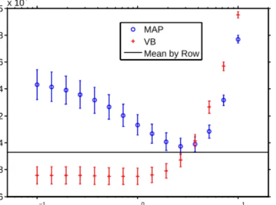
Figure 3: Predictive loss computed on the binarized BusStop dataset to illustrate the automatic smoothing of the VB the algorithm compared to MAP estimation. The hori-zontal axis is the amount of regularization, i.e.c−2u,k=c−2v,k.
For each dataset, we generated a binary version of the data by setting to one any strictly positive count. For the count data, we removed 5% of the highest values to obtain a reasonable value for ymax. We used logistic regression (i.e. sigmoid inverse link function) to model binary ob-servations and Poisson potentials (3) where based on the λ(x) = log(1 +ex)inverse link function. Our goal is data imputation: predicting the values of missing entries in a
count matrix. We evaluate our predictions using the likeli-hood of the test data, i.e. the logistic loss
`(y,ˆx) =ylog(ˆx) + (1−y) log(1−xˆ)
for binary data and the asymmetric Poisson loss: `(y,xˆ) =λ(ˆx)−ylog
x
λ(ˆx)
,
for count data, wherey is the true value andxˆ is the pre-diction.
Implementation details For binary data, we used the lo-gistic regression inverse link function, and for count data, we used the novel rate functionλ(x) = log(1 +ex) pre-sented earlier. The prior variances c2
u,k,c2v,k of the latent factors where set to be equal and their value was selected in the range[0.1,10]and the dimensionKof the latent fac-tors varied from 1 to 5. For each dataset, we selected these hyperparameters by optimizing the performance on a val-idation data matrix, which was not used in the subsequent experiments. The training times quoted below do not in-clude these validation runs. Our implementation is written in Matlab. Computations were run on a standard 8-core Linux server.
Baseline algorithm We compare against MAP estima-tion. As noted there, the MAP algorithm has a similar structure to our VB method, where the G-VBMF subrou-tine simply shrinks and threshold at 0 the eigenvalues, by a amount directly proportional toc−2u,k andc−2v,k. Note that the singular value thresholding step in the MAP algorithm corresponds to the solution of a nuclear-norm regularized problem with spherical Gaussian likelihood.
In all our experiments, convergence speed is similar to EM-like algorithms: the train EM-likelihood quickly increases with the first iterations, but the algorithm is extremely slow to converge to the exact maximum values. In any case, after approximately 100 iterations, the test likelihood does not increase significantly. In all the experiments, we stopped after a maximum of 200 iterations. One can see expample of learning curves for various values of the latent dimension
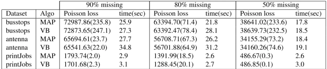
90% missing 80% missing 50% missing Dataset Algo Poisson loss time(sec) Poisson loss time(sec) Poisson loss time(sec) busstops MAP 72987.86(235.8) 25.9 63394.70(71.4) 21.8 38641.02(233.6) 17.8 busstops VB 72873.65(247.1) 27.3 63392.47(78.4) 28.1 38639.73(232.5) 18.5 antenna MAP 65694.61(23.7) 27.7 56708.71(67.3) 26.2 34155.29(73.2) 18.4 antenna VB 65541.63(22.0) 34.8 56701.88(64.9) 31.2 34160.26(74.6) 19.1 printJobs MAP 1793.74(2.0) 2.9 1391.99(18.5) 2.6 486.67(0.3) 2.6 printJobs VB 1701.68(2.3) 3.1 1288.45(20.1) 2.7 486.85(0.1) 3.0
Table 2: Test log-likelihood of the MAP estimator and the proposed VB algorithm for count data on various data sets with different proportion of missing data. Results are averaged over 10 runs (standard deviation in parenthesis).
in Figure 2. Results on binary data are shown in Table 1, while results on count data based on Poisson potentials are shown in Table 2. VB predictions generally outperform those of MAP estimation, indicating that Bayesian averag-ing over uncertainties helps in our data imputation tasks, especially when the fraction of missing data is large. When the matrix is nearly full (i.e. with 50% of missing data), the MAP solution and the VB solution tend to become equiva-lent. Note also that the runtime of our VB method is close to that of MAP, showing that the additional computation involved in the G-VBMF subroutine is negligible.
6
Conclusions
We presented a novel efficient algorithm for variational Bayesian inference in general matrix factorization mod-els with non-conjugate Poisson and Bernoulli likelihoods. Based on the analytical solution for fully observed spher-ical Gaussian likelihood Matrix Factorization models de-rived in [9], our method is driven by few calls to approx-imate SVD solvers for “sparse plus low rank” matrices, in contrast to previous VB alternate minimization algo-rithms which typically require many iterations and restarts to avoid poor local optima. We employ Poisson poten-tials for count or discrete score data, proposing a novel in-verse link function with better properties than the canoni-cal exponential choice. Our method can be scanoni-caled to very large problems using standard software available in Mat-lab. It outperforms MAP estimation on a range of real-world problems, while running in time comparable to a highly efficient MAP solver which employs SVD shrink-age in a similar manner.
In future work, we aim to use more sophisticated local variational bounds, while maintaining the reduction to G-VBMF. Specifically, we are not yet using the degrees of freedom offered by thecu,k,cv,k parameters in G-VBMF. Also, we are working on a improvement on the bound by relaxing the constraint of having a constant varianceκ ac-cross all the observations, as done for heteroscedastic ma-trix factorization [1]: by using local variational bounds valid for every row rather than for the whole matrix, one can obtain tighter bound. A simple rescaling of the latent
matrix rowsX=UVT, would then lead to the same sub-problem solved by the G-VBMF. This idea could equiva-lently be applied to the columns of the matrix, but it is not clear how to do it jointly in rows and columns, in order to be efficient on large and nearly squared matrices.
References
[1] Lakshimanarayan B., G. Bouchard, and C. Archambeau. Robust Bayesian matrix factorisation. In G. Gordon and D. Dunson, editors,Workshop on Artificial Intelligence and Statistics 14, 2011.
[2] J. Cai, E. Candes, and Z. Shen. A singular value thresh-olding algorithm for matrix completion. SIAM J. Optim., 20:1956–1982, 2008.
[3] O. Chapelle and Z. Harchaoui. A machine-learning ap-proach to conjoint analysis. In Saul et al. [16], pages 257– 264.
[4] S. Deerwester, S. Dumais, G. Furnas, R. Landauer, and R. Harshman. Indexing by latent semantic analysis.Journal of the American Society for Information Science, 41(6):391– 407, 1990.
[5] T. Jaakkola. Variational Methods for Inference and Estima-tion in Graphical Models. PhD thesis, Massachusetts Insti-tute of Technology, 1997.
[6] E. Khan, B. Marlin, G. Bouchard, and K. Murphy. Varia-tional bounds for mixed-data factor analysis. In Y. Bengio, D. Schuurmans, J. Lafferty, C. K. I. Williams, and A. Cu-lotta, editors, Advances in Neural Information Processing Systems 22. Curran Associates, 2009.
[7] J. Konstan, B. Miller, D. Maltz, J. Herlocker, L. Gordon, and J. Riedl. Grouplens: Applying collaborative filtering to usenet groups. Communications of the ACM, 40(3):77–87, 1997.
[8] Y. Lim and Y.-W. Teh. Variational Bayesian approach to movie rating prediction. InProceedings of KDD Cup and Workshop, 2007.
[9] S. Nakajima and Sugiyama. Theoretical analysis of Bayesian matrix factorization. Journal of Machine Learn-ing Research, 12:2579–2644, 2011.
[10] L. Paninski, J. Pillow, and E. Simoncelli. Maximum likeli-hood estimation of a stochastic integrate-and-fire neural en-coding model.Neural Computation, 16:2533–2561, 2004. [11] T. Raiko, A. Ilin, and J. Karhunen. Principal component
analysis for large scale problems with lots of missing values. In J. Kok, J. Koronacki, R. Lopez, S. Matwin, D. Mladenic, and A. Skowron, editors,European Conference on Machine Learning 18, pages 691–698. Springer, 2007.
[12] M. Rattray, O. Stegle, K. Sharp, and J. Winn. Inference algo-rithms and learning theory for Bayesian sparse factor anal-ysis. Journal of Physics: Conference Series, 197(012002), 2009.
[13] G. Reinsel and R. Velu.Multivariate Reduced-Rank Regres-sion: Theory and Applications. Springer, 1st edition, 1998.
[14] R. Rosipal and N. Kr¨amer. Overview and recent advances in partial least squares. InSubspace, Latent Structure and Feature Selection Techniques. Springer, 2006.
[15] R. Salakhutdinov and A. Mnih. Probabilistic matrix factor-ization. In J. Platt, D. Koller, Y. Singer, and S. Roweis, ed-itors, Advances in Neural Information Processing Systems 20, pages 1257–1264. Curran Associates, 2008.
[16] L. Saul, Y. Weiss, and L. Bottou, editors.Advances in Neu-ral Information Processing Systems 17. MIT Press, 2005. [17] N. Srebro, J. Rennie, and T. Jaakkola. Maximum margin
matrix factorization. In Saul et al. [16], pages 1329–1336.
[18] M. Tao and X. Yuan. Recovering low-rank and sparse com-ponents of matrices from incomplete and noisy observa-tions.SIAM J. Optim., 21(1):57–81, 2011.
[19] M. Tipping and C. Bishop. Probabilistic principal compo-nent analysis. Journal of Roy. Stat. Soc. B, 61(3):611–622, 1999.
[20] R. Tomioka, T. Suzuki, M. Sugiyama, and H. Kashima. An efficient and general augmented Lagrangian algorithm for learning low-rank matrices. In J. F¨urnkranz and T. Joachims, editors,International Conference on Machine Learning 27, pages 1087–1094. Omni Press, 2010.