Multi-Step Approach to Improving Accuracy of Incident Duration Estimation: Case Study
of Istanbul
Halit OZEN, Abdulsamet SARACOGLU
Abstract: Unexpected events, such as crashes, disabled vehicles and spilled loads cause traffic congestion or increase the level of existing congestion on roads. Traffic incident management requires the estimation of incident duration from the beginning to the final stage of the event, in order to identify the most suitable strategies for decreasing their impact. Accordingly, the adverse effects of an incident can be minimised by efficiently managing the process between the time the incident occurred and the traffic returning to normal operating conditions. The purpose of this paper is to present a methodology and improve the accuracy of the model by using a multi-step approach to estimate the duration of an incident. For this purpose, incident duration data was obtained for Istanbul Transit Europe Motorways (TEM). Using the incident data and implementing the multi-step approach, Kalman Filtering and linear regression analysis in stepwise, were used for the incident duration estimation model.
Keywords: incident duration; Kalman Filter; linear regression; multi-step approach; traffic incident 1 INTRODUCTION
One of the major problems encountered in the operation of highways in large urban areas is traffic congestion. Traffic congestion often occurs in segments where demand is greater than capacity and emerges in two different ways, recurring and non-recurring. For recurring congestion, which regularly occurs in peak hour traffic every day, travellers would be able to plan their journey according to expected congestion; even so, non-recurring congestion originated by traffic incidents (accidents, vehicle breakdowns, debris, for example), results in unexpected congestion on the carriageway. Therefore, road users cannot take this congestion into account when planning a journey unless they have been told about the incident before they start travelling.
Within the scope of this study, an incident duration estimation model was established using Kalman Filtering and linear regression analysis and the incident data that occurred on the Istanbul TEM. In the second section, studies in the literature regarding traffic incident duration estimation were investigated. Details of the data are given in the third section. In the following section, methodology and the methods used in the study are discussed. The established forecasting model and corresponding results are evaluated in the fifth section. In the last section, results of the study are presented and recommendations are made.
2 LITERATURE REVIEW
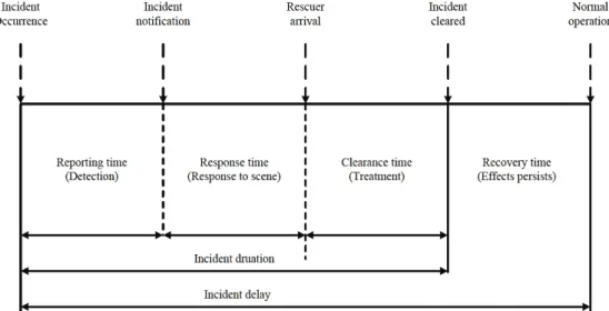
Taking into account studies regarding incident duration estimation, in general, the process of a traffic incident is examined in four time intervals, partitioned with five time points [1, 2]. These points are, chronologically: incident occurrence, incident notification, response unit arrival, incident clearance, and normal operation. The first three time intervals between these points are expressed as the total incident duration [3-5], and all four time intervals are expressed as the total delay caused by the incident [1, 2].
As seen in Fig. 1, the stages of the incident are detection time, response time, clearance time and, recovery time [1, 2]. Due to the difficulty in defining the precise starting time of an incident, in some research the time
interval between incident notification and incident clearance is called modified incident duration [6, 7].
Incident delay and incident duration can vary, depending on factors such as environmental conditions and the nature of the incident. By determining these characteristics, incident duration can be estimated using statistical forecasting methods. Accuracy of incident duration estimations depends on the quality of the collected data, incident characteristics and the estimation methods. The quality of the data declines due to an insufficient number of data and its being collected from only one source. On the other hand, different incident characteristics and environmental components can be used to estimate the incident duration, such as the type of incident (crash, debris, breakdown etc.), time, location, number of vehicles involved in the incident, category of vehicle, number of lanes affected by the incident, injury and death toll, the number of heavy vehicles involved in the incident, cargo spilled, weather conditions and damage to road equipment. In addition to the nature of the incident, traffic demand data for the segment of road on which the incident occurred should be known at the time of the incident to establish a model for incident delay, including recovery time [8-10].
Also the estimation method used for incident duration could have a significant effect on the accuracy of the estimated incident duration. In previous research studies, various statistical methods and data mining techniques have been used, including the classification tree method [1], artificial neural networks [4, 6], linear regression [5, 8], hazard based analysis model [2, 10, 11], cyclic subspace regression [12], support vector regression [13], partial least squares regression [7, 14], time series method [15], fuzzy logic model [16] and Bayesian Networks approaches [17-19].
Garib et al. [8], analysed 277 incidents and six different incident characteristics for estimating incident duration in the USA. Accordingly, they performed regression analysis with lognormal distribution and found the estimating accuracy of the incident duration to be 81%. Özbay & Noyan made the other USA study [17]. They used the Bayesian Network method and 650 incident data for estimating the incidents’ clearance time. By using seven model inputs and 10 test datasets generated by dividing the
whole dataset, estimating the accuracy of incident duration was 81%, following 10 iterations.
Chung [3], established a Hazard Based incident duration estimation model by analysing 4869 incidents in South Korea. The average error of estimation was found to be 18 minutes and the Mean Absolute Percentage Error (MAPE) was calculated to a reasonable value of 47%.
Lopes et al. [6] analysed 10762 incidents that occurred in Portugal between 2008 and 2011. They estimated the clearance time of incidents using Artificial Neural Networks. As a result, after testing the model with 244 incidents that occurred in 2011, the model estimated 72% with an error of less than 10 minutes and 92% with an error of less than 20 minutes.
Figure 1 Traffic incident time intervals and points
Figure 2 Study flow chart Wang et al. [7], established four models, using four
different regression types. For estimating incident duration, they used 1853 incidents that occurred in Netherlands. The models acquired the best accuracy of prediction to be 83,6%, 92,7%, and 88,2% at error for 20 minutes, for stopped vehicle, lost-load and accident, respectively.
According to above-mentioned studies, in literature, traffic incident duration is generally estimated in a single step. However, a multi-step approach, whose estimated duration in the first step is used as input to the subsequent
step, is expected to increase accuracy. On the other hand, Kalman Filtering is used in many fields in the literature including traffic incident detection in traffic incident management studies but estimation of incident duration [20]. Thus, in this study, the multi-step approach, whose estimated duration in the Kalman Filtering Analysis is used as input to the Multi Linear Regression Analysis is proposed.
3 METHODOLOGY
The multi-step approach was used for the estimation of the incident duration. The study flow chart is given in Fig 2. As seen in Fig. 2, the necessary data was obtained from the General Directorate of Highways Traffic Operation Centre (GDH-TOC) and analysed the video streaming and the images to collect the incident characteristic data [21]. A data cleaning process was applied to exclude outliers from the data set. Pearson Correlation was conducted to investigate a relationship between the incident characteristics. Kalman filter estimation was run for each significant variable to calculate the initial incident duration. Linear regression conducted using the initial incident duration as an independent variable, was the output of the Kalman Filtering Analysis, while the incident duration is the dependent variable.
Kalman Filtering is a theory developed by Rudolf Kalman in 1960. It is primarily used in weather forecasting. Kalman filtering makes predictions based on present and previous data. For instance a ship travelling between destinations A and B finds its way with the help of GPS. If the GPS stops working, the Kalman filtering approach can be used to calculate a route based on the previous routing data [22].
The Kalman filter is an efficient recursive computational method to predict or estimate the state of a process. It is based on a set of mathematical equations that try to minimize the mean squared error and it works on a so-called prediction-correction approach [23]. In the first step of the Kalman Filtering Analysis, Eq. (1) and Eq. (2) are used for making predictions.
1 1
k k k k
x = ⋅A x− + ⋅B u +w − (1)
k k k
Z =H⋅x +v (2)
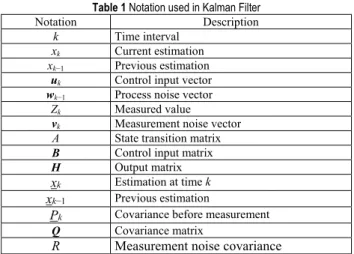
Each xk can be evaluated by using linear stochastic equation. Any estimated incident duration (xk) is a combination of its previous value estimated plus a control signal uk and noise. Zk is a measured value that consists of a linear combination of xk and vk. The notation used in Kalman Filtering is illustrated in Tab. 1.
Table 1 Notation used in Kalman Filter
Notation Description
k Time interval
xk Current estimation
xk−1 Previous estimation
uk Control input vector
wk−1 Process noise vector
Zk Measured value
vk Measurement noise vector
A State transition matrix
B Control input matrix
H Output matrix
xk Estimation at time k
xk−1 Previous estimation
Pk Covariance before measurement Q Covariance matrix
R Measurement noise covariance
The second step of the Kalman Filtering Analysis is the iteration (prediction-correction mechanism). The filter estimates the process state at a given value and then obtains feedback in the form of (noise) measurements. The main equations in Kalman Filtering and the working process are presented in Fig. 3. As seen in Fig. 3, Kalman filter iteration equations are divided into two groups, as follows: prediction and correction. The prediction equations are responsible for projecting forward the current state and error covariance estimates to obtain the a priori estimates for the next step. The correction equations are used for integrating new measurements into a previous estimate to obtain an improved a posteriori estimate [23].
Figure 3 Kalman Filtering steps
4 DATA DESCRIPTION
Within the scope of this study, data from the GDH-TOC was used for incidents that occurred on the Istanbul TEM for the 12 months between October 1, 2013 and September 30, 2014, including recorded streaming and
images [21]. Data includes the following information about the incidents: date, time, vehicle type, number of vehicles, location, severity, detection time, response time, clearance time and response units. Recorded streaming and images were examined to gather new characteristics about the incidents. Characteristics that were gathered by analysing
the recorded streaming and images included, accident type, number of lanes, lane blockage, lane(s) that accident occurred, number of heavy vehicles, road condition (wet or dry), cargo spillage, liquid spillage and damage to road equipment.
For reliability, short time incidents of less than five minutes that did not have an effect on traffic flow and incident data that had uncertain characteristics were excluded from the data set. Consequently, the total of 2517 incident data was reduced to 1151, the number of incident data that was used in this study.
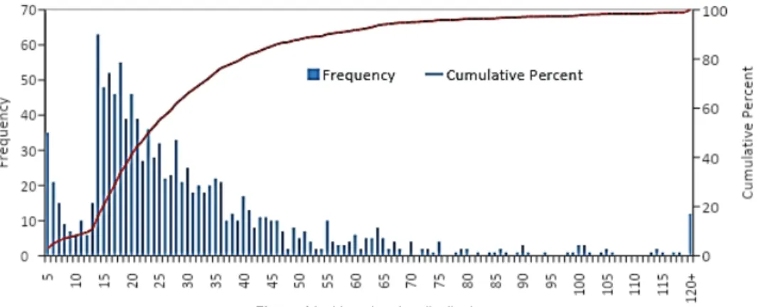
As can be seen from the distribution of incident duration presented in Fig. 4, the mean duration is 30,34 minutes and approximately 92% of these incidents were
under 60 minutes. Also, standard deviation is 24,86 minutes with an extreme right-skewed distribution and the maximum duration was 260 minutes. There were 12 incidents that had a duration of more than 120 minutes and the duration was 14 minutes for more than 60 incidents.
In the study, 15 different variables regarding incidents that could possibly have affected the incident duration were taken into consideration. The effect of each variable on incident duration was established by correlation analysis using the Pearson coefficient and is presented in Tab. 2. According to Tab. 2, five of the 15 variables, including what part of the week, season, number of vehicles, number of heavy vehicles and the road condition are insignificant for incident duration, so these variables were not used for the estimation.
Figure 4 Incident duration distribution
Table 2 Results of Pearson Correlation analysis
Accidents Characteristics Coefficient P-Value Part of Week 0,024 0,412 Season -0,037 0,205 Part of Day 0,084 0,004* Location -0,113 0,000* Severity 0,259 0,000* Type 0,243 0,000* Number of Lanes -0,124 0,000* Lane -0,079 0,008* Lane Blockage 0,088 0,003* Number of Vehicles 0,025 0,389 Number of Heavy Vehicles 0,050 0,089** Road Condition (Dry/Wet) 0,039 0,181
Cargo Spill 0,284 0,000*
Liquid Spill 0,389 0,000*
Damage Equipment 0,290 0,000*
* Significant at 95% confidence level; ** Significant at 90% confidence level; Coefficients which are statistically significant at 95% level or greater are in bold.
5 ANALYSIS RESULTS
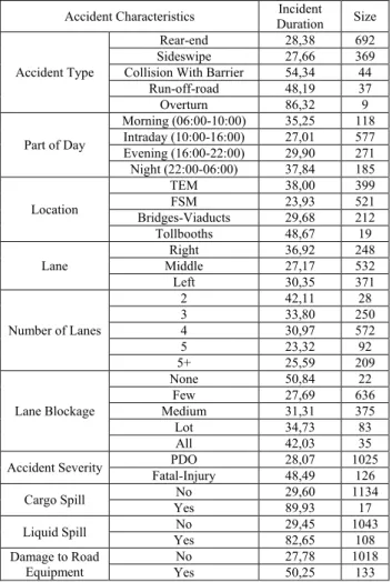
The Kalman Filtering approach is applied with respect to different incident characteristics and new incident durations, that were found, are presented in Tab. 3.
On the TEM, the highway that is analysed in this study, heavy vehicles are prohibited from using it during peak periods. Therefore, accident data is separated according to different times of the day, based on the time of the accident. The heavy vehicle restriction periods are 06:00-10:00 AM and 04:00-10:00 PM and are called Morning and Evening restriction periods, respectively. The other periods, during which there are no heavy vehicle restrictions, are 10:00 AM - 04:00 PM, called Intraday and 10:00 pm - 06:00 am, called Night period. At night and during the morning
period, incident duration is above 35 minutes; by contrast, it is less than 30 minutes for the intraday and the evening period.
When data was analysed with respect to types of accident, maximum incident duration was for those involving overturned vehicles. On the other hand, incident duration was less than 30 minutes for rear-end and sideswipe accidents. Accidents are divided into four parts, based on the location of the incident. The part including FSM Bridge and its tollbooths was named FSM; similarly, the remaining parts of the TEM highway were named TEM. But the response time to the accidents at bridges, viaducts and tollbooths are quite different. For this reason Bridges-Viaducts and Tollbooths were classified separately. FSM Bridge was found to be the location with the lowest incident duration. This section can be reopened to traffic flow 24 minutes after the occurrence of an accident. Also, incident duration is less than half an hour for other accidents that happened on bridges and viaducts, except the FSM Bridge. Bridges and viaducts are critical points on the highway and have frequent traffic controls, so incident duration is low at these segments.
Based on the number of lanes at the sections where an accident occurs, incident duration at segments with 5 and 5+ lanes is found to be approximately 25 minutes. Frontage roads with 2 lanes that run parallel to the main road have the highest incident duration, which is about 42 minutes. On the other hand, accidents that occurred in the right lane occupied the incident site for longer than either the left or middle lane.
The blockage percentages of the lanes were calculated by dividing the number of blocked lanes at the incident location by the total number of lanes. Based on these
percentages, the data is divided into five parts; none (0%), few (0-33%), medium (33-67%), many (67-100%), all (100%). According to the blockage percentages of the lanes, incident duration is highest for ‘none’. For the other accidents, incident duration increased gradually, with increasing blockage percentages. On the other hand, incident duration of injury-fatal accidents is more than PDO accidents.
Table 3 Results of Kalman Filtering approach with respect to different accident characteristics
Accident Characteristics Duration Incident Size Accident Type
Rear-end 28,38 692 Sideswipe 27,66 369 Collision With Barrier 54,34 44
Run-off-road 48,19 37 Overturn 86,32 9 Part of Day Morning (06:00-10:00) 35,25 118 Intraday (10:00-16:00) 27,01 577 Evening (16:00-22:00) 29,90 271 Night (22:00-06:00) 37,84 185 Location TEM 38,00 399 FSM 23,93 521 Bridges-Viaducts 29,68 212 Tollbooths 48,67 19 Lane Middle Right 36,92 27,17 248 532
Left 30,35 371 Number of Lanes 2 42,11 28 3 33,80 250 4 30,97 572 5 23,32 92 5+ 25,59 209 Lane Blockage None 50,84 22 Few 27,69 636 Medium 31,31 375 Lot 34,73 83 All 42,03 35 Accident Severity Fatal-Injury PDO 28,07 48,49 1025 126
Cargo Spill Yes No 29,60 89,93 1134 17 Liquid Spill Yes No 29,45 82,65 1043 108 Damage to Road
Equipment Yes No 27,78 50,25 1018 133 Accident data was also analysed according to factors such as the spilling of cargo, spilling of liquids (for example fuel and oil) and the existence of any damage to road equipment. According to this evaluation, spilling of cargo, spilling of liquid and the existence of damage to
road equipment, increased the incident duration dramatically.
By using the Kalman Filtering approach with respect to different accident characteristics, incident duration is estimated for each incident data. A scatter graph of the actual and estimated value of each incident is shown in Fig 5. As seen in Fig. 5, the Kalman Filtering approach underestimated incident duration and the accuracy of the estimation needs to be improved.
For the evaluation of the model accuracy, mean absolute percentage error (MAPE), root mean square error (RMSE), standard deviation and average value of estimated values were calculated.
The RMSE basically provides an estimate of error variance. The normal variance measures the distance from the mean of a data set. However, RMSE measures the variance from 0, which should be an ideal error for any prediction. The RMSE can be computed by taking the sum of the squares of the errors (difference between the predicted and actual values), computing the average and then taking the square root (Eq. (3)) [20].
(
)
21 ( ) ( )
N t
predicted value t actual value t RMSE
N =
−
=
∑
(3)The mean absolute percentage error (MAPE) is a summary measure widely used for evaluating the accuracy of prediction results, and it is expressed as follows (Eq. (4)):
(
)
1 ( ) ( ) 1 ( ) N tactual value t predicted value t
MAPE
N = actual value t
−
=
∑
(4)The lower the MAPE value, the more accurate the prediction model is. Listed in Tab. 4 is a scale rating for evaluating the accuracy of a model based on the MAPE method, as developed by Lewis [3].
Table 4 Scale of evaluation of prediction accuracy
MAPE Assessment Less than 10% Highly accurate prediction
11% to 20% Good prediction 21% to 50% Reasonable prediction 51% or more Inaccurate prediction
Figure 5The scatter graph of the actual value and the estimated values withKalman Filtering As presented in Tab. 5, results of the Kalman Filtering
As seen in Tab. 5, for all the methods that implemented the Kalman Filtering approach, RMSE values are higher than average values and if the duration is more than 25 minutes the error of the models and accuracy of the models is unsatisfactory for incident management, as shown in Fig. 5. Therefore, to increase the model’s accuracy, linear
regression analysis has been applied to estimate the incident duration, using the Kalman Filtering estimation results. Actual incident duration values were selected as a dependent value while the Kalman Filtering estimated values were selected as independent values. Results of the linear regression analysis are illustrated in Tab. 6.
Table 5 Evaluating accuracy of Kalman Filtering approach
Method RMSE (min) MAPE (%) Standard Deviation (min) Average (min)
Kalman Filtering Approach
Part of Day 24,47 37,55 6,43 16,19 Location 23,87 37,19 6,84 16,41 Severity 23,99 36,10 7,45 16,71 Type 23,40 36,88 7,72 16,57 Number of Lanes 24,53 37,66 6,31 16,13 Lane 24,54 37,55 6,28 16,13 Lane Blockage 24,43 37,52 6,60 16,20 Cargo Spill 23,87 37,54 6,95 16,18 Liquid Spill 23,85 37,45 7,03 16,23 Damage Equipment 23,78 36,71 7,25 16,54
Table 6 Results of Linear Regression Analysis
Coefficients P-value Constant -19,73 0,00* Part of Day (X1) -0,22 0,41 Location (X2) 2,70 0,00* Severity (X3) -0,63 0,00* Type (X4) 0,27 0,10** Number of Lanes (X5) -0,98 0,01* Lane (X6) -0,01 0,97 Lane Blockage (X7) -0,48 0,02* Cargo Spill (X8) 1,80 0,00* Liquid Spill (X9) 0,20 0,56 Damage Equipment (X10) 0,41 0,02*
* Significant at 95% confidence level; ** Significant at 90% confidence level; Coefficients which are statistically significant at 95% level or greater are in bold.
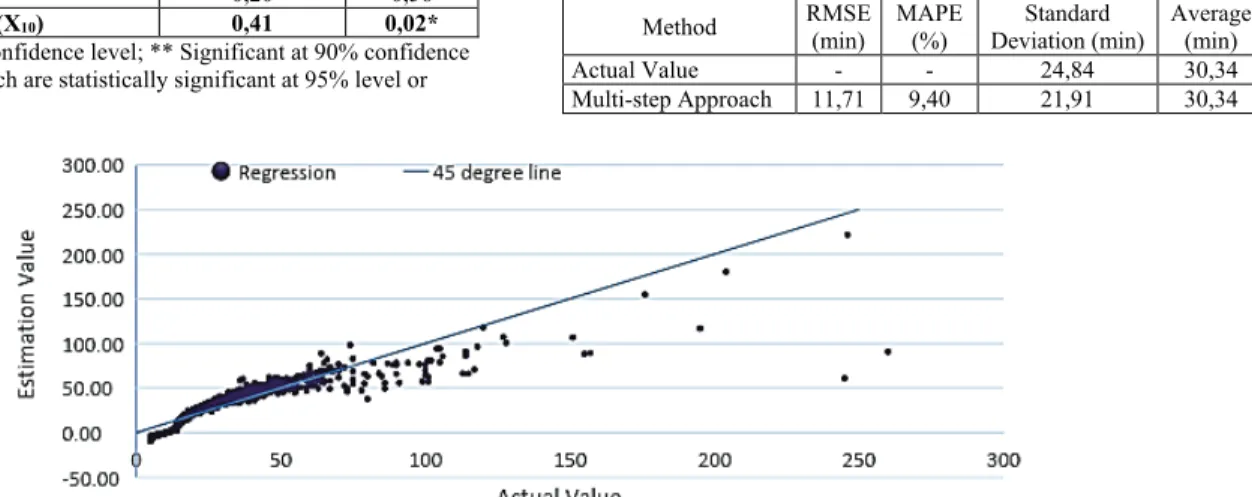
The scatter graph of the actual and the estimated values calculated with a multi-step approach are depicted in Fig. 6.
Results of the multi-step approach are given in Tab. 7. If the results are compared with the Kalman Filtering estimation method (Tab. 5), a significant improvement can be seen in the mean of the MAPE (9,40%) and the RMSE (11,71 min).
Table 7 Evaluating accuracy of Multi-Step Approach
Method RMSE (min) MAPE (%) Deviation (min) Standard Average (min) Actual Value - - 24,84 30,34 Multi-step Approach 11,71 9,40 21,91 30,34
Figure 6 The scatter graph of the actual value and the estimated values with Multi-Step Approach
6 CONCLUSIONS AND RECOMMENDATIONS
Throughout this study, data on traffic accidents that occurred in Istanbul have been evaluated. By using incident data and the multi-step approach to implementing the step wise Kalman Filtering and linear regression analysis, the incident duration estimation model has been established. The RMSE value of the incident duration for Kalman Filtering is approximately 24 minutes, but it is 12 minutes for the multi-step approach. Therefore, the accuracy of the multi-step approach is two times higher than the estimation of the incident duration using Kalman Filtering. In conclusion, the offered model can be considered as a useful tool to estimate incident duration for Istanbul.
It is possible to increase the accuracy of the estimations by adding new parameters, such as the number of fatalities
and injuries, the location of the closest response unit and weather conditions.
Even so, in order to provide effective incident management, studies relating to incident duration estimation should be improved. It is possible to determine those aspects that will be affected by an accident and imply new strategies for incident management, which will result in a decrease in the negative impact of these incidents.
Acknowledgements
The authors would like to thank Koksal Avincan for his valuable discussions.
7 REFERENCES
[1] Chang, H. L. & Chang, T. P. (2013). Prediction of freeway incident duration based on classification tree analysis.
Journal of the Eastern Asia Society for Transportation Studies, 10, 1964-1977. https://doi.org/10.11175/easts.10.1964 [2] Chung, Y. (2010). Development of an accident duration
prediction model on the Korean freeway systems. Accident Analysis and Prevention, 42, 282-289.
https://doi.org/10.1016/j.aap.2009.08.005
[3] Nam, D. & Mannering, F. (2000). An exploratory hazard-based analysis of highway incident duration. Transportation Research Part A, 34, 85-102.
https://doi.org/10.1016/S0965-8564(98)00065-2
[4] Wei, C. H. & Lee, Y. (2007). Sequential forecast of incident duration using artificial neural network models. Accident Analysis and Prevention, 39, 944-954.
https://doi.org/10.1016/j.aap.2006.12.017
[5] Shin, C. H. (2003). Development of freeway incident duration prediction models. Journal of the Eastern Asia Society for Transportation Studies, 5, 1734-1744. Retrieved from http://www.easts.info/2003journal/index.html [6] Lopes, J., Bento, J., Pereira, F. C., & Akiva, M. B. (2012).
Dynamic forecast of incident clearance time using adaptive artificial neural network models. Proceedings of the 92nd
TRB Annual Meeting Compendium of Papers. Retrieved
fromhttp://trid.trb.org/view.aspx?id=1242255
[7] Wang, X., Chen, S., & Zheng, W. (2013). Analysis of regression method on traffic incident duration. Proceedings of the ASCE 2013 International Conference on Transportation Information and Safety, 1008-1015.
https://doi.org/10.1061/9780784413036.136
[8] Garib, A., Radwan, A. E., & Al-Deek, H. (1997). Estimating magnitude and duration of incident delays. Journal of Transportation Engineering, 123, 459-466.
https://doi.org/10.1061/(ASCE)0733-947X(1997)123:6(459)
[9] Sullivan, E. C. (1997). New model for predicting freeway incidents and incident delays. Journal of Transportation Engineering, 123, 267-275.
https://doi.org/10.1061/(ASCE)0733-947X(1997)123:4(267)
[10] Hojati, A. T., Ferreira, L., Washington, S., Charles, P., & Shobeirinejad, A. (2014). Modelling total duration of traffic incidents including incident detection and recovery time. Accident Analysis and Prevention, 71, 296-305.
https://doi.org/10.1016/j.aap.2014.06.006
[11] Chimba, D., Kutela, B., Ogletree, G., Horne, F., & Tugwell, M. (2014). Impact of abandoned and disabled vehicles on freeway incident duration. Journal of Transportation Engineering, 140(3), 04013013(8).
https://doi.org/10.1061/(ASCE)TE.1943-5436.0000635
[12] Xuanqiang, W., Shuyan, C., Jian, G. U., & Wenchang, Z. (2013). Traffic incident duration analysis based on cyclic subspace regression. Proceedings of the ASCE 2013 Fourth International Conference on Transportation Engineering, 2854-2860.https://doi.org/10.1061/9780784413159.414
[13] Wu, W., Chen, S., & Zheng, C. (2011). Traffic incident duration prediction based on support vector regression. Proceedings of the ASCE 2011 Eleventh International Conference of Chinese Transportation Professionals, 2412-2421. https://doi.org/10.1061/41186(421)241
[14] Wang, X., Chen, S., & Zheng, W. (2013). Traffic incident duration prediction based on partial least squares regression. Procedia - Social and Behavioral Sciences, 96, 425-432. https://doi.org/10.1016/j.sbspro.2013.08.050
[15] Khattak, A. J., Schofer, J. L., & Wang, M. H. (1995). A simple time sequential procedure for predicting freeway incident duration. IVHS Journal, 2(2), 113-138.
https://doi.org/10.1080/10248079508903820
[16] Wang, W., Chen, H., & Bell, M. (2002). A study of the characteristics of traffic incident duration on motorways. Traffic and Transportation Studies, 1101-1108.
https://doi.org/10.1061/40630(255)153
[17] Ozbay, K. & Noyan, N. (2006). Estimation of incident clearance times using Bayesian networks approach. Accident Analysis and Prevention, 38, 542-555.
https://doi.org/10.1016/j.aap.2005.11.012
[18] Park, H., Haghani, A., & Zhang, X. (2013). Interpretation of Bayesian neural network for predicting the duration of detected incidents. Journal of Intelligent Transportation Systems: Technology, Planning, and Operations, 20(4), 385-400. https://doi.org/10.1080/15472450.2015.1082428
[19] Yang, B. J., Zhang, X., & Sun, L. (2008). Traffic incident duration prediction based on the Bayesian decision tree method. Proceedings of the First International Symposium on Transportation and Development Innovative Best Practices, 338-343. https://doi.org/10.1061/40961(319)56 [20] Škorput, P., Mandžuka, S., & Jelušić, N. (2010). Real-time
detection of road traffic incidents. Promet-Traffic & Transportation, 22(4), 273-283.
https://doi.org/10.7307/ptt.v22i4.192
[21] General Directorate of Highways Traffic Operation Centre (2013). Traffic incident report database,Istanbul.
[22] Dogan, G. & Avincan, K. (2017). MultiProTru: A Kalman Filtering based trust architecture for two-hop wireless sensor networks. Peer-to-Peer Networking and Applications, 10(1), 278-291.https://doi.org/10.1007/s12083-016-0446-3
[23] Bayraktar, M. E., Arif, F., Ozen, H., & Tuxen, G. (2015). Smart parking-management system for commercial vehicle parking at public rest areas. Journal of Transportation Engineering, 141(5),04014094(16)
https://doi.org/10.1061/(ASCE)TE.1943-5436.0000756
Contact information:
Halit OZEN, PhD, Associate Professor Yildiz Technical University,
Faculty of Civil Engineering,
Department of Transportation Engineering, Davutpasa Campus, Esenler, Istanbul, Turkey E-mail: [email protected]
Abdulsamet SARACOGLU, MSc, Research Assistant
Yildiz Technical University, Faculty of Civil Engineering,
Department of Transportation Engineering, Davutpasa Campus, Esenler, Istanbul, Turkey E-mail: [email protected]