Approximating the Nondominated Front Using the Pareto Archived Evolution Strategy

the Pareto Archived Evolution Strategy

Joshua D. Knowles

School of Computer Science, Cybernetics and Electronic Engineering

University of Reading Reading RG6 6AY, UK [email protected]

David W. Corne

School of Computer Science, Cybernetics and Electronic Engineering

University of Reading Reading RG6 6AY, UK [email protected]

Abstract

We introduce a simple evolution scheme for multiobjective optimization problems, called the Pareto Archived Evolution Strategy (PAES). We argue that PAES may represent the simplest possible nontrivial algorithm capable of generating diverse solutions in the Pareto optimal set. The algorithm, in its simplest form, is a (1+1) evolution strategy employing

local search but using a reference archive of previously found solutions in order to identify the approximate dominance ranking of the current and candidate solution vectors. (1+1

)-PAES is intended to be a baseline approach against which more involved methods may be compared. It may also serve well in some real-world applications when local search seems superior to or competitive with population-based methods. We introduce (1+

)

and (

+

) variants of PAES as extensions to the basic algorithm. Six variants of PAES

are compared to variants of the Niched Pareto Genetic Algorithm and the Nondominated Sorting Genetic Algorithm over a diverse suite of six test functions. Results are analyzed and presented using techniques that reduce the attainment surfaces generated from several optimization runs into a set of univariate distributions. This allows standard statistical analysis to be carried out for comparative purposes. Our results provide strong evidence that PAES performs consistently well on a range of multiobjective optimization tasks. Keywords

Genetic algorithms, evolution strategies, multiobjective optimization, test functions, mul-tiobjective performance assessment.

1 Introduction

Multiobjective optimization using evolutionary algorithms has been investigated by many authors in recent years (Bentley and Wakefield, 1997; Fonseca and Fleming, 1995a; Horn et al., 1994; Horn and Nafpliotis, 1994; Parks and Miller, 1998; Schaffer, 1985; Srinivas and Deb, 1994). However, in some real-world optimization problems, the performance of the genetic algorithm is overshadowed by local search methods such as simulated annealing and tabu search, either when a single objective is sought or when multiple objectives have been combined by the use of a weighted sum (see Mann and Smith (1996)). This suggests that multiobjective optimizers that employ local search strategies would be promising to inves-tigate and compare with population-based methods. Good results have been obtained with such methods (Czyzak and Jaszkiewicz, 1998; Gandibleux et al., 1996; Hansen, 1997, 1998; Serafini, 1994; Ulungu et al., 1995), and, recently, some theoretical work has been done which yields convergence proofs for simple variants (Rudolph, 1998a, 1998b). However,

it is currently unclear how well local-search based multiobjective optimizers compare with evolutionary algorithm based approaches. Here, we introduce a novel evolutionary al-gorithm called the Pareto Archived Evolution Strategy (PAES) that, in its baseline form, employs local search for the generation of new candidate solutions but utilizes population information to aid in the calculation of solution quality. The algorithm, as presented here, has three forms: (1+1)-PAES, (1+

)-PAES, and (

+

)-PAES.

Evolution Strategies (ESs) were first reported by Rechenberg (1965) following the seminal work of Peter Bienert, Ingo Rechenberg, and Hans-Paul Schwefel at the Technical University of Berlin in 1964. A modern and comprehensive introduction is in B¨ack (1996). We find the (

+

) model of ESs to naturally fit the general structure of PAES and the

variants used in this paper, but we should note that we use neither the adaptive step sizes for mutation nor the encoding of strategy parameters that are usually associated with ESs. There is no reason, of course, why these may not be included in further variants of PAES, perhaps in investigations with real-valued encodings.

Six test functions are used to compare PAES to two well-known and respected multiobjective genetic algorithms (MOGAs) – the Niched Pareto Genetic Algorithm (NPGA) (Horn et al., 1994; Horn and Nafpliotis, 1994) and the Nondominated Sort-ing Genetic Algorithm (NSGA) (Srinivas and Deb, 1994). Four of the test problems have been previously used by several researchers (Bentley and Wakefield, 1997; Horn et al., 1994; Horn and Nafpliotis, 1994; Fonseca and Fleming, 1995a; Schaffer, 1985), and the fifth is a new problem devised by us as a further challenge to find diverse Pareto optima. The aim of this comparison is to explore and demonstrate the applicability of the PAES approach to standard multiobjective problems. Our sixth problem, the Adaptive Distributed Database Management Problem (ADDMP), is strictly a real-world application but is included as a test problem because we provide resources to allow other researchers to carry out the exact same optimization task. Analysis of all the results generated has been carried out using a comparative/assessment technique put forward by Fonseca and Fleming (1995b). This works by transforming the data collected from several runs of an optimizer into a set of univariate distributions. Standard statistical techniques can then be used to summarize the distributions or to compare the distributions produced by two competing optimizers. We compare pairs of optimizers using the Mann-Whitney rank sum test (for example, see Mendenhall and Beaver, 1994) as our statistical comparator.

1.1 Overview of the Paper

The remainder of the paper is organized as follows. In Section 2, we introduce PAES and its components. Pseudocode describing both the basic (1+1) algorithm and the archiving

strategy is presented. A crowding procedure used by PAES is also described. Finally, the time complexity of PAES is estimated and a discussion of the (1+

) and (

+

)

variants is provided. Section 3 describes our set of test problems. Four of these are well-known test problems in the multiobjective literature, and two are new. One of the new ones is a contrived problem that, when encoded with

k

genes that can each take any of

k

integer values, has

k

Pareto optima. It is a considerable challenge on this problem for a multiobjective algorithm to find any of these

k

Pareto optima, let alone find a good spread. The second new test problem, for which we also provide the fitness function and other details via a website, is a multiobjective version of the Adaptive Distributed Database Management Problem. This is a two-objective problem in which the objectives involved relate to quality-of-service issues in the management of a distributed database. In Section 4

we describe the algorithms compared in later experiments. These are three algorithms based on NPGA, four based on NSGA, and six versions of PAES (with differing

and

). Section 5 is devoted to a discussion of the statistical comparison method we use, based on Fonseca and Fleming’s seminal ideas on this topic. Section 6 presents the results, and we conclude in Section 7.

2 The PAES Algorithm

2.1 Motivations

PAES was initially developed as a multiobjective local search method for finding solutions to the off-line routing problem (Mann and Smith, 1996; Knowles and Corne, 1999), which is an important problem in the area of telecommunications routing optimization. Previous work on this problem used single-objective (penalty-function) methods, and it was found that local search was generally superior to population-based search. PAES was, therefore, developed to see if this finding carried over into a multiobjective version of the off-line routing problem. A comparison of early versions of PAES with a more classical MOGA on the off-line routing problem is provided in Knowles and Corne (1999). The positive findings of this earlier work prompted the investigation of the performance of PAES on a broader range of problems presented here.

2.2 (1+1)-PAES

The (1+1)-PAES algorithm is outlined in Figure 1. It is instructive to view PAES as

comprising three parts: the candidate solution generator, the candidate solution acceptance function, and the nondominated-solutions (NDS) archive. Viewed in this way, (1+1)-PAES

represents the simplest nontrivial approach to a multiobjective local search procedure. The candidate solution generator is akin to simple random mutation hillclimbing; it maintains a single current solution and, at each iteration, produces a single new candidate via random mutation.

1 generate initial random solution

c

and add it to the archive

2 mutate

c

to produce

m

and evaluate

m

3 if (

c

dominates

m

) discard

m

4 else if (

m

dominates

c

)

5 replace

c

with

m

, and add

m

to the archive

6 else if (

m

is dominated by any member of the archive) discard

m

7 else apply test(

c

,

m

,archive) to determine which becomes the new

current solution and whether to add

m

to the archive

8 until a termination criterion has been reached, return to line 2

Figure 1: Pseudocode for (1+1)-PAES.

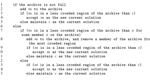
Since the aim of multiobjective search is to find a spread of nondominated solutions, PAES needs to provide an NDS list to explicitly maintain a limited number of these, as and when they are found by the hillclimber. The design of the acceptance function is obvious in the case of the mutant dominating the current solution or vice versa but is troublesome in the nondominated case. Our approach is to learn from Horn et al.’s seminal work (Horn et al., 1994; Horn and Nafpliotis, 1994) and hence use a comparison set to help decide between the mutant and the current solution in the latter case. The NDS archive provides a natural and convenient source from which to obtain comparison sets. Pseudocode indicating the

1 if the archive is not full

2 add

m

to the archive

3 if (

m

is in a less crowded region of the archive than

c

)

4 accept

m

as the new current solution

5 else maintain

c

as the current solution

6 else

7 if (

m

is in a less crowded region of the archive than

x

for

some member

x

on the archive)

8 add

m

to the archive, and remove a member of the archive from

the most crowded region

9 if (

m

is in a less crowded region of the archive than

c

)

10 accept

m

as the new current solution

11 else maintain

c

as the current solution

12 else

13 if (

m

is in a less crowded region of the archive than

c

)

14 accept

m

as the new current solution

15 else maintain

c

as the current solution

Figure 2: Pseudocode for test(

c

,

m

,archive).

procedure for determining whether to accept or reject the mutant solution and for deciding whether it is archived or not is given in Figure 2.

Arguably, even simpler multiobjective local search procedures are possible. One might have a simpler acceptance function, which always accepts the mutant unless the current solution dominates it. Or, it could only accept the mutant if it dominates the current solution. We tried both of these, however, and found the results to be very poor. Echoing Horn et al.’s findings, we found that the use of a nontrivially sized comparison set is crucial to reasonable results.

We note that the idea of maintaining a list of nondominated solutions is not new. Parks and Miller (1998) recently describe a MOGA that also maintains an ‘archive’ of nondominated solutions. In their case, the overall algorithm is much more complicated than PAES, and the archive is not just used as a repository and a source for comparisons but also plays a key role as a pool of possible parents for selection. They found the use of this archive gave improved results over a traditional MOGA, tested on a particular application. They do not provide results (but indicate this as a future direction) on the use of their MOGA+‘archive’ method on standard or other multiobjective test problems, however.

2.3 Adaptive Grid Algorithm

An integral part of PAES is the use of a new crowding procedure based on recursively dividing up the

d

-dimensional objective space. This procedure is designed to have two advantages over the niching methods used in some multiobjective GAs: Its computational cost is lower; it is adaptive so that it does not require the critical setting of a niche-size parameter.

When each solution is generated, its grid location in objective space is determined. Assuming the range of the space is defined in each objective, the required grid location can be found by repeatedly bisecting the range in each objective and finding in which half the solution lies. The location of the solution is recorded as a binary string of length2

l

d

, where

l

is the number of bisecitons of the space carried out for each objective, and

d

is

the number of objectives. Each time the solution is found to be in the larger half of the prevailing bisection of the space, the corresponding bit in the binary string is set. A map of the grid is also maintained, indicating for each grid location how many and which solutions in the archive currently reside there. We choose to call the number of solutions residing in a grid location itspopulation. The use of the population of each grid location forms an important part of the selection and archiving procedure outlined in Figure 2. Notice that with an archive size of 100, for example, and a two-objective problem with

l

=5, phenotype

space is divided into 1024 squares. However, the archive is naturally clustered into a small region of this space, representing the slowly advancing approximation to the Pareto front, and the entire archive will perhaps occupy some 30 to 50 squares.

The recursive subdivision of the space and assignment of grid locations is carried out using an adaptive method that eliminates the need for a niche size parameter. This adaptive method works by calculating the range in objective space of the current solutions in the archive and adjusting the grid so that it covers this range. Grid locations are then recalculated. This is done only when the range of the objective space of archived solutions changes by a threshold amount to avoid recalculating the ranges too frequently. The only parameter that must then be set is the number of divisions of the space (and hence grid locations) required.

The time complexity of the adaptive grid algorithm, in terms of the number of com-parisons which must be made, may be derived from the population size

n

, the number of solutions currently in the archive

a

, the number of subdivision levels being used

l

, and the number of objectives of the problem

d

. Finding the grid location of a single solution requires

l

d

comparisons. Thus, finding the grid location of the whole archive requires

a

l

d

(1)

comparisons. Updating the quadtree ranges requires, in the worst case, that the whole population is added to the archive and, thus, that the whole population must be compared to the current maximum and minimum values in each of the

d

dimensions. Therefore, this updating can take up to

2

d

n

+

n

l

d

(2)

comparisons. This gives a worst case time order of

O

((

a

+

n

)

d

)comparisons 1

per iteration. In practice, the grid locations of the archive only need updating infrequently as few solutions outside the current range of the archive will be found per generation2

. Furthermore, rarely will more than one or two new points join the archive per generation, and so the average case number of comparisons to update the quadtree ranges is far fewer than the worst case given in Equation 2. Niching, by contrast, requires

n

(

n

?1)comparisons per generation

and significant additional overhead if calculating Euclidean distances between each pair of points. In the case where niching is carried out on the partially filled next generation, as in Horn and Nafpliotis (1994), niching still requires

n

2

(

n

+1)comparisons, which is also

O

(

n

2

).

1

Note we have removedlas it will, in general, be small, especially ifdis large. For example, in a three-objective

problem, we require onlyl=5to give us(2 5

) 3

=32768divisions of the search space. 2

Generation, here, refers to an iteration of the PAES algorithm. For example, in (1+)-PAES,new solutions

2.4 The Time Complexity of PAES

(1+1)-PAES is a simple, fast algorithm when compared against MOGAs of similar

per-formance (see Section 6). Here, we analyze its time complexity in terms of the number of comparisons that must be carried out per generation of the algorithm. We compare PAES with NPGA and NSGA on the two core processes of selection and acceptance.

Selection is not required at all in (1+1)-PAES since there is only one current solution.

Therefore, all of the complexity is involved in the acceptance/rejection of the mutant solution and the updating of the archive. In this process, PAES requires1comparison to

compare the candidate solution with the current solution and a further

a

d

comparisons

(in the worst case) to compare the current solution with the archive, where

a

is the current archive size and

d

is the number of objectives in the problem. It requires

l

d

to find the

candidate’s grid location. A further2

d

comparisons are required to update the quadtree

ranges and another

a

l

d

comparisons if the archive grid locations require updating.

The best and average case complexity of PAES is significantly different from the worst case outlined above, however. It requires only

d

comparisons to ascertain that the candidate solution is dominated by the current solution, and in this case, no further comparisons are required in that generation. Similarly, if the candidate is dominated by anything in the archive, no updating of the quadtree ranges or grid locations is necessary. In PAES the latter case occurs frequently since the archive represents a diverse sample of the best solutions ever found. In many cases, for example, the archive is not full, i.e.,

a <

arcmax

, where

arcmax

is the maximum size of the archive. So, as soon as one of the members of the archive is found to dominate the candidate, no further comparisons are required. Thus, in the average case, the number of comparisons required to reject a candidate is much smaller than

arcmax

d

. These considerations show that PAES is a very aggressive search method.

It wastes little time on solutions that turn out to be substandard, instead concentrating its efforts only on solutions that are comparable to the best ever found.

The NSGA requires no comparisons in the replacement of the current population by the next generation. Instead, the complexity of this algorithm comes from the assignment of fitness values required for selection to be carried out. The number of comparisons in the nondominated sorting phase is given by

rn

(

n

?1), where

r

is the number of dominance

ranks found in the population. The niche count phase then requires

n

(

n

?1) further

comparisons. Unlike PAES, NSGA requires this number of comparisons every generation regardless of the quality of the solutions generated; thus, its worst case performance equals its best case performance.

Similarly, the NPGA employs

cn

comparisons for selection, where

c

is the comparison set size. If niching is then carried out on the partly filled next generation, then each time a tie occurs between the two or more candidate solutions in the tournament, a further

n

next

t

comparisons must be made, where

n

next

is the number of solutions currently in the next generation and

t

is the number of solutions that tied. In the worst case, this means that

t

size

(

n

+1)

n

2

comparisons are made per generation if, each time, the tournament is tied between all the candidate solutions in the tournament. On average, the niching process will require significantly fewer comparisons than this, however.

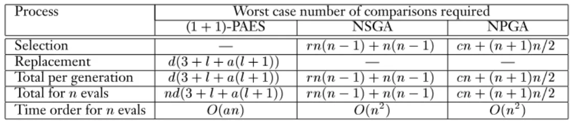
The above analysis is summarized in Table 1. Rows four and five of the table indicate the number of comparisons required by each algorithm (worst case) and their overall time order, respectively, to evaluate

n

solutions. This brings (1+1)-PAES into line with the two

Table 1: Time complexity involved in selection and replacement phases. Process Worst case number of comparisons required

(1+1)-PAES NSGA NPGA

Selection —

rn

(

n

?1)+

n

(

n

?1)

cn

+(

n

+1)

n=

2

Replacement

d

(3+

l

+

a

(

l

+1)) — —

Total per generation

d

(3+

l

+

a

(

l

+1))

rn

(

n

?1)+

n

(

n

?1)

cn

+(

n

+1)

n=

2

Total for

n

evals

nd

(3+

l

+

a

(

l

+1))

rn

(

n

?1)+

n

(

n

?1)

cn

+(

n

+1)

n=

2

Time order for

n

evals

O

(

an

)

O

(

n

2

)

O

(

n

2

)

PAES presents the same number of final solutions as the MOGAs, then all three algorithms are

O

(

n

2

)in the number of comparisons required to evaluate

n

solutions. However, because

of the aggressiveness of PAES, its average case number of comparisons is significantly less than the two MOGAs that expend the same amount of effort on poor solutions as they do on good ones. The computational requirements of these algorithms are further illustrated in Section 6, where we present their computation times for one selected problem.

2.5 (1+

)-PAES and (

+

)-PAES

The (1+1)-PAES serves as a good, simple baseline algorithm for multiobjective

optimiza-tion. Its performance is strong, especially given its low computational complexity, even on demanding tasks where one might expect local search methods to be at a disadvantage (see Section 6). However, in this paper we also investigate the performance of (1+

) and (

+

)

variants of it.

The generation of

mutants of the current solution increases the problem of deciding which one to accept as the next current solution(s). This is, in fact, carried out by assigning a fitness to each mutant based upon both a comparison with the archive and its grid location population.

Each of the

+

population members is compared to the archive as it appeared after the last iteration and is assigned adominance scoreas follows. Its score is initially zero and is set to 1 if it finds an archive member that it dominates. A score of 0 indicates it is nondominated by the archive. If it is dominated by any member of the archive, its score is set to -1, and no more comparisons are necessary. All mutants that could potentially join the archive are used to recalculate the ranges of the phenotype space. If this has changed by more than a threshold amount, then the grid locations of the archive and potential archive members are recalculated. The archive is then updated. Finally, a fitness is assigned to each population member such that members with a higher dominance score are always given a higher fitness regardless of their grid location population. Points of the same dominance score have higher fitness the lower the population of their grid location.

Updating of the archive occurs as in (1+1)-PAES, ensuring that it contains only

nondominated solutions and no copies. If it becomes full, then solutions in sparse regions of the space will be favored. This ensures that the comparison set covers a diverse range of individuals so that the dominance score assigned to population members reflects their true quality.

In (

+

)-PAES, the

mutants are generated by mutating one of the

current

in the previous iteration.

3 The Test Problems

We have compared PAES with the NPGA and NSGA on a suite of standard test functions. Each defines a number of objectives that are to be minimized simultaneously. The first four of these are the same as used by Bentley and Wakefield (1997): Schaffer’s functions

F

1,

F

2, and

F

3, and Fonseca’s

f

1 (Fonseca and Fleming, 1995a), renamed here as

F

4.

These functions are now commonly used by researchers to test multiobjective optimization algorithms. For reasons noted next, we also designed an additional test function called

F

5.

F

1is a single-objective minimization problem with one optimum:

f

1 =

x

1 2 +

x

2 2 +

x

3 2 (3)

F

2is a two-objective minimization problem with a single range of Pareto optima that

lie in0

x

2:

f

21 =

x

2

f

22 = (

x

?2) 2 (4)

F

3 is two-objective minimization problem with two separate ranges of Pareto optima

that lie in1

x

2and4

x

5:

f

31 = ?

x

where

x

1 = ?2+

x

where 1

< x

3 = 4?

x

where 3

< x

4 = ?4+

x

where 4

< x

f

32 = (

x

?5) 2 (5)

F

4 is a two-objective minimization problem on two variables with a single range of

Pareto optima running diagonally from(?1

;

1)to(1

;

?1):

f

41 = 1?

e

(?(

x

1?1) 2 ?(

x

2+1) 2 )

f

42 = 1?

e

(?(

x

1+1) 2 ?(

x

2?1) 2 ) (6)

The above test functions are useful in testing multiobjective optimizers because they implicitly set two challenges. First, the set of nondominated solutions delivered by the optimizer should contain all of the function’s Pareto optima. Second, it is generally felt best if there is no strong bias favoring one Pareto optimum over others. In other words, in a MOGA, for example, the number of copies of each Pareto optimum in the final population should be similar. If not, this would seem to reveal a bias that may be undesirable in practical applications.

We designed

F

5(described below) to provide stronger challenges in these respects; it

is easily defined but is a nontrivial problem. Each Pareto optimum is intrinsically difficult to find, and there are

k

distinct Pareto optima for chromosomes of length

k

, each having a different frequency, i.e., some are far easier to find than others. This makes both challenges (as described above) stringent tests for any multiobjective optimizer.

The function

F

5uses a

k

-ary chromosome of

k

genes. There are two objectives to be

minimized, defined by the following two functions:

f

51 =

k

?1?

k

?2 X

i

=0 1 if

G

i

+1 ?

G

i

=1 0 otherwise (7)

f

52 =

k

?1?

k

?2 X

i

=0 1 if

G

i

?

G

i

+1 =1 0 otherwise (8)

where

G

i

is the allele value of the

i

th gene. For example, a chromosome of length

k

=5

with allele values ‘1 2 3 2 2’ scores5?1?2=2for the first objective (because there are

two sites where, reading the chromosome from left to right, the allele value increases by exactly 1) and5?1?1=3for the second objective, using similar reasoning. From this,

we can see that the best score possible for either objective is0, the worst is

k

?1, and the

Pareto front is formed by solutions for which

f

51 +

f

52

=

k

?1.

3.1

F

6: The Adaptive Distributed Database Management Problem

The Adaptive Distributed Database Management Problem (ADDMP) has been described in several places. Space constraints preclude a full description here, but a detailed description is in Oates and Corne (1998). C source code for the evaluation function of the ADDMP and data for the test problem we use here can be found via the first author’s website3

. In this article, we will limit our description of the ADDMP to providing its basic details, aimed at conveying an understanding of the context in which a multiobjective tradeoff surface arises. The ADDMP is an optimization problem from the viewpoint of a distributed database provider. For example, providers of video-on-demand services, on-line mailing-list brokers, and certain types of Internet service providers, all need to regularly address versions of the ADDMP. The database provider must ensure that good quality service is maintained for each client, and the usual quality of service measure is the delay experienced between a database query and the response to that query.

At a snapshot in time, each client will experience a typical delay depending on current traffic levels in the underlying network and on which database server the client’s queries are currently routed to. The database provider is able to reconfigure the connections at intervals. For example, the database provider might re-route client 1’s queries to server 7, client 2’s queries to server 3, client 3’s queries to server 7, and so on. The ADDMP is the problem of finding an optimal choice of client/server connections given the current client access rates, basic server speeds, and general details of the underlying communications matrix. An optimal configuration of such connections is clearly one that best distributes the access load across servers, allowing for degradation of response as the load on a server increases, and other issues.

Test function

F

6 is an example instance of the ADDMP involving ten nodes (each is

both a client and a server) and in which quality of service is measured by two objectives, both of which must be minimized. The first objective is the worst response time (measured in milliseconds) seen by any client. This is clearly something that a database provider needs to minimize by reconfiguration. However, it is insufficient as a quality of service measure by itself. For example, if we have just three clients, then a situation in which the response

3

times are respectively 750ms, 680ms, and 640ms will appear better, with this quality of service measure, than if the response times were 760ms, 410ms, 300ms. To achieve a more rounded consideration of quality of service, we look at the tradeoff between this objective and another: the mean response time of the remaining (non-worst) clients. Hence, the two scenarios in this example would yield the following nondominated points: (750, 660), (760, 355).

4 The Algorithms

In the remainder of this paper, we wish to establish the performance characteristics of several different forms of the PAES algorithm on a number of test functions. In order to do this, we use as comparison two of the most well-known and respected MOGAs: NPGA and NSGA. In order to give each algorithm an equal opportunity of generating a good set of diverse solutions we add two extensions to the genetic algorithms:

1. An archive of the nondominated solutions found is maintained (as in PAES) for pre-sentation at the end of a run.

2. Elitism is employed.

The archive is not used to aid in selection, acceptance, or any other part of the GA—it is merely there to give the GA the same opportunity as PAES to present the best solutions it has found. Elitism is implemented as follows: In the case of the NSGA, this is straight-forward as fitness values are assigned, and we can merely place into the new population the

g

fittest solutions, where

g

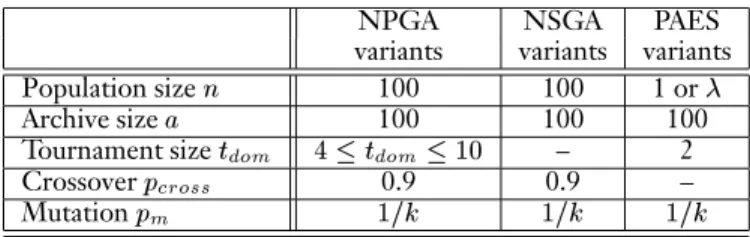
is the generation gap parameter. Thus, the NSGA has four different variants: the standard NSGA without elitism or archiving (NSGA), the NSGA with archiving (NSGA+ARC), the NSGA with elitism (NSGA+ELITE), and the NSGA with both elitism and archiving (NSGA+A+E). Elitism cannot be carried out easily in the Niched Pareto GA, however, because explicit fitness values are never assigned. Thus, we have only three variants of the Niched Pareto GA. These are the standard Niched Pareto GA (NPGA), the NPGA with archiving (NPGA+ARC), and the NPGA with archiving and elitism (NPGA+A+E). The latter works by placing all individuals that were archived in the previous generation into the next generation.

Each of the algorithms require two or more parameter values to be set. Due to space restrictions a complete discussion regarding these choices cannot be included here. Instead, they are summarized in Table 2.

Table 2: Summary of algorithm parameters.

NPGA NSGA PAES

variants variants variants

Population size

n

100 100 1 or

Archive size

a

100 100 100

Tournament size

t

dom

4

t

dom

10 – 2

Crossover

p

cross

0.9 0.9 –

Mutation

p

m

1

=k

1

=k

1

=k

The NPGA uses the simple triangular sharing function

Sh

[

d

] = 1?

d=

share

for

between two solutions. We find that the NPGA requires a fairly large comparison set size in order for its estimate of the dominance ranking of individuals to remain fairly accurate. Similarly, the tournament size cannot be set too low if accurate selection is to occur. Values of

cs

size

=80and tournament size10

t

dom

4are usually acceptable. The niche size

parameter

share

must also be set. Here, some experimentation is required as the NPGA can be quite sensitive to this parameter. So, for each of the problems attempted, several test runs were undertaken to find reasonable values for the niche count parameter and the tournament size.

The nondominated sorting GA requires fewer parameters to be set. To set the niche size parameter, several test runs were carried out to obtain reasonable performance. In our elitist variants of the NSGA, we must also set the number of solutions

g

to be carried through to the next generation. In all experiments,

g

=5was used.

With the exception of test problem

F

5, uniform crossover was used in both of the

above MOGAs. Single point crossover is more suited to finding solutions in

F

5, and this

was used, again, in both MOGAs. Values of crossover probability

p

cross

=0

:

9were used in

both MOGAs, and a bit flip mutation rate

p

m

=1

=k

for a chromosome of

k

genes was used

in all of the algorithms including PAES. In addition, (

+

)-PAES requires a tournament

size for selection. For this, a value of

t

dom

=2was found to be acceptable on all problems.

5 Statistical Comparison of Multiobjective Optimizers

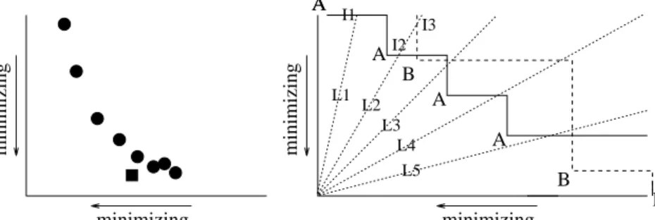
Proper comparison of results from two multiobjective optimizers is a complex matter. Instead of comparing two distributions of scalar values (one from each algorithm), as in the single objective case, we need to compare two distributions of approximations to the Pareto front. Often, results from different multiobjective optimizers have been compared via visual observation of scatter plots of the resulting point. One recent step towards a more formal and statistical approach was made and used by Zitzler et al. (1999) using a ‘coverage’ metric. In this method, the resulting set of nondominated points from a single run of algorithm

A

and another from a single run of algorithm

B

are processed to yield two numbers: the percentage of points from algorithm

A

that are equal to or dominated by points from

B

, and vice versa. Statistical tests are performed on the numbers yielded from several such pairwise comparisons. However, this method is quite sensitive to the way in which points may or may not be clustered in different regions of the Pareto surface as illustrated in Figure 3(left). In the figure, one algorithm returns the set of points indicated by circles, and the other returns the single point indicated by a square. The coverage metric would score 0% for the first algorithm and 50% for the second. However, the first clearly returns a better approximation to the Pareto tradeoff surface than the second, albeit further from the optimal Pareto surface than the second algorithm in one region.

A statistical comparison method proposed by Fonseca and Fleming (1995b) addresses this and other issues. It works as illustrated in Figure 3(right). The resulting approximations to the Pareto surface from two algorithms

A

and

B

are shown by appropriately labeled points. The lines joining the points (solid for

A

, dashed for

B

) indicate the attainment surfaces. An attainment surface divides phenotype space into two regions; one containing points that dominate or are nondominated by points returned from the algorithm, and another containing all points dominated by the algorithm’s results. Fonseca and Fleming’s idea was to consider a collection of sampling lines that intersect the attainment surfaces across the full range of the Pareto frontier. Examples of such lines are indicated by L1-L5

A A A A A B B L1 L2 L3 L4 L5 I1 I2 I3 B minimizing minimizing minimizing minimizing

Figure 3: Problems with the coverage metric (left); sampling the Pareto frontier using lines of intersection (right).

in the figure. Line L1, for example, intersects

A

’s attainment surface at I1 and will intersect with

B

’s attainment surface somewhere above the figure at a place far more distant from the origin than I1. Line L2 intersects

A

’s attainment surface at I2, and

B

’s at I3; again,

A

’s intersection is closer to the origin.

Given a collection of

k

attainment surfaces, some from algorithm

A

and some from algorithm

B

, a single sampling line yields

k

points of intersection, one for each surface. These intersections form a univariate distribution, and we can, therefore, perform a sta-tistical test to determine whether or not the intersections for one of the algorithms occurs closer to the origin with some statistical significance. Such a test is performed for each of several lines covering the Pareto tradeoff area (as defined by the extreme points returned by the algorithms being compared). Insofar as the lines provide a uniform sampling of the Pareto surface, the result of this analysis yields two numbers—the percentage of the surface in which algorithm

A

outperforms algorithms

B

, and the percentage of the surface in which algorithm

B

outperforms algorithm

A

—both calculated with respect to the chosen level of statistical significance. For example, if repeated runs of the two algorithms of Figure 3(left) produced identical or similar results to the two runs indicated, the result of this test would be around [60,40], indicating that the first algorithm outperforms the second on about 60% of the Pareto surface, while the second outperforms the first on around 40% of the surface. A more common result in practice is that the two numbers sum to rather less than 100, indicating that no significant conclusion can be made with respect to many of the sampling lines.

1 initialize:

a

=

b

=

nlines

= 0

2 for each sampling line

L

3 for each attainment surface

s

in

S

A

S

S

B

4 find the intersection of

L

with

s

5 statistically analyzes the distribution of intersections

6 if (

A

outperforms

B

on

L

with required significance)

then

a

++

7 if (

B

outperforms

A

on

L

with required significance)

then

b

++

8

nlines

++

9 return the result: [100*

a

/

nlines

, 100*

b

/

nlines

]

Figure 4 indicates the comparison method in pseudocode for a collection of attainment surfaces

S

A

and

S

B

from two algorithms

A

and

B

. The idea is first described in Fonseca and Fleming (1995b), but we next include extra details that may benefit others intending to implement it. In particular, our code for this comparison method is available from the website given earlier and capable of performing the comparisons as described for any number of objectives. Space limitations preclude a full description of the method here, for example, precisely how we define the lines and how we find the intersections of multidimensional lines with multidimensional attainment surfaces. However, interested readers are referred to the available C code and contact with the authors to see how this is done.

As indicated, we find that a good way to present the results of a comparison is in the form of a pair [

a

,

b

], where

a

gives the percentage of the space (i.e., the percentage of lines) on which algorithm

A

was found statistically superior to

B

, and

b

gives the similar percentage for algorithm

B

. Typically, if both

A

and

B

are ‘good’,

a

+

b <

100. The

result100?(

a

+

b

)then, of course, gives the percentage of the space on which results were

statistically inconclusive. We present all of our results in this form.

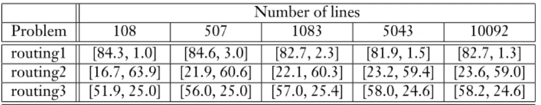
For the number of lines, we find that 100 is adequate, although, obviously, the more lines the better. We will use as an example our experiments on three different versions of the off-line routing problem which illustrate this (see note at beginning of Section 2, Mann and Smith (1996), and Knowles and Corne (1999)). This particular choice of problem is of interest here since it involves three objectives. The NPGA and (1+1)-PAES algorithms tailored for this problem (see Knowles and Corne (1999)) were compared on each of three versions of it. Table 3 gives the results using variable numbers of lines.

Table 3: PAES vs NPGA comparisons with differing numbers of lines. Number of lines

Problem 108 507 1083 5043 10092

routing1 [84.3, 1.0] [84.6, 3.0] [82.7, 2.3] [81.9, 1.5] [82.7, 1.3] routing2 [16.7, 63.9] [21.9, 60.6] [22.1, 60.3] [23.2, 59.4] [23.6, 59.0] routing3 [51.9, 25.0] [56.0, 25.0] [57.0, 25.4] [58.0, 24.6] [58.2, 24.6]

In Table 3, we can see that the general trend as we use more lines is that a greater percentage of the space is found to give statistically significant results. (Note, in these cases and all others in the paper, we use statistical significance at the 95% confidence). This trend is not perfect, however. For example, on the routing1 problem, the 1083-line sample indicates that PAES was superior to the NPGA on 82.7% of the space, but the situation is reversed on a further 2.3% of the space, with a further 15.0% of the space giving inconclusive results. When we sample the space in approximately five times as many places (5043 lines), 16.7% of the space returns inconclusive results. Such variation as we change the number of lines can be explained by the kind of situation we see in Figure 3(right), where

B

’s attainment surface ‘bulges’ through

A

’s between lines L2 and L3. If such a bulge was very small in relation to the distance between lines, then it may affect the results (if sampled) but perhaps with more prominence than it deserves. A greater number of lines, hence sampling more in the region around the bulge, would reveal that it really was quite small, suitably leading to a reduction in its effect on the results.

This is the most appropriate among the set of standard statistical tests, since the data are essentially unpaired, and it avoids assuming that the distributions are Gaussian. However, it does assume that the distributions of intersections for the two algorithms are of the same shape. We have not tested this assumption in the cases reported here. Intuitively, we would expect the assumption to be sufficiently true for variants of the same algorithm (such as (

+

)-PAES for different

and

), but less so for, say, a comparison between (1+1)-PAES

and NPGA. We are addressing this detail in further work on extending the comparison technique.

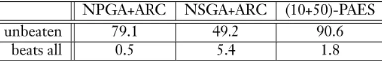
Finally, we also do comparisons on multiple (more than two) sets of points from multiple algorithms. Results for such comparisons are presented in Table 4.

Table 4: Three MOGAs compared on Schaffer’s function

F

3.

NPGA+ARC NSGA+ARC (10+50)-PAES

unbeaten 79.1 49.2 90.6

beats all 0.5 5.4 1.8

In such a comparison of

k

algorithms, the comparison code performs pairwise statistical comparisons, as before, for each of the

k

(

k

?1)

=

2distinct pairs of algorithms. The results

then show, for each algorithm, on what percentage of the space we can be statistically confident that it was unbeaten by any of the other

k

?1algorithms and on what percentage

of the space it beat all

k

?1algorithms. For example, in Table 4, we can see that the

archived version of NPGA was unbeaten on 79.1% of the space covered by the three algorithms compared. That is, on 79.1% of the space, no algorithm was found superior at the 95% confidence level.

6 Results and Discussion

6.1 The Test Problems

Each algorithm tested was allowed the same number of function evaluations,

max evals

, on each of the test problems. Following a number of trial runs to obtain good parameter settings, twenty uniquely seeded runs were carried out, and the resulting solution sets recorded. For each test function, the number of function evaluations allowed and the length of the chromosome

k

are given in Table 5.

Table 5: The allowed number of function evaluations and chromosome length for each of the six test functions.

F

1

F

2

F

3

F

4

F

5

F

6

max evals

1000 5000 5000 20000 20000 5000

k

16 14 14 16 16 10

The single objective test problem

F

1 presents no difficulty to any of the optimizers

Table 6: Comparison of three variants of the Niched Pareto GA.

NPGA+ARC NPGA+A+E (1+1)-PAES

F

2- Schaffer’s function

F

2 NPGA [0, 97.0] [0, 98.4] [0, 96.2] NPGA+ARC — [7.1, 9.6] [11.0, 7.6] NPGA+A+E — — [10.9, 4.1]

F

3- Schaffer’s function

F

2 NPGA [0, 99.5] [0, 99.4] [0, 99.0] NPGA+ARC — [4.9, 1.0] [0.9, 13.0] NPGA+A+E — — [0.2, 19.3]

F

4- Fonseca’s function

f

1 NPGA [0, 100] [0, 100] [0, 100] NPGA+ARC — [12.8, 1.3] [12.8, 1.6] NPGA+A+E — — [2.9, 8.6]

F

5-

k

-optima problem NPGA [0, 100] [0, 100] [0, 100] NPGA+ARC — [93.6,0] [34.7, 48.2] NPGA+A+E — — [0, 100]

F

6- the ADDMP NPGA [0, 99.8] [0, 98.0] [0, 95.7] NPGA+ARC — [0.4, 0] [6.6, 90.0] NPGA+A+E — — [2.2, 89.5]

return, in their archive, the single nondominated solution only. The three GA versions employing archiving exhibit the same behavior, as expected. When no archive is used, the population of both the NPGA and the NSGA converge to this solution, subject to random mutations in the last generation. Because

F

1presents no difficulty to any of the optimizers

here and is not itself a multiobjective problem, no further discussion or results relating to this problem are presented.

For each of the remaining five problems, tests were carried out in the following way: First, all of the NPGAs were compared, in pairs, one against the other (and also against (1+1)-PAES as a baseline), each time taking the combined space of the pair as the range

over which to test, and using the statistical techniques outlined in Section 5. Next, in the same way, the NSGAs and the PAES algorithms were internally compared. From these three sets of internal tests, we chose the best NPGA, NSGA, and PAES algorithm and compared these in the same fashion. Sometimes it was not clear from the original tests which algorithm in the initial groups should be carried forward to the ‘final’. Where this happens, further internal tests were performed and/or two inseparable algorithms were both carried forward for inclusion in the final. Finally, the combined space ofallthe algorithms was used and

n

(

n

?1) comparisons were performed on the

n

= 13algorithms. Again,

results were collected in terms of the percentages of the space on which each algorithm was unbeaten and beat all. Readers are reminded that all comparisons use a Mann-Whitney rank-sum test at the 95% confidence level.

Table 7: Comparison of six variants of the Pareto Archived Evolution Strategy. (1+10)-PAES 1+50 10+1 10+10 10+50

F

2- Schaffer’s function

F

2 (1+1)-PAES [5.8, 2.1] [17.1, 1.4] [12.7, 1.4] [3.9, 5.4] [5.3, 3.7] 1+10 — [16.8, 1.8] [9.3, 2.8] [1.1, 6.8] [4.2, 5.7] 1+50 — — [4.3, 10.4] [0.8, 24.5] [1.6, 19.9] 10+1 — — — [1.1, 16.5] [1.7, 10.9] 10+10 — — — — [6.1,4.7]

F

3- Schaffer’s function

F

3 (1+1)-PAES [9.5, 0.9] [10.0, 0] [11.6, 0.7] [3.3, 1.4] [5.2, 0.8] 1+10 — [3.1, 1.8] [2.5, 1.2] [0.6, 6.5] [1.3, 55.3] 1+50 — — [2.0, 3.3] [0.1, 8.2] [0.2, 45.3] 10+1 — — — [0.7, 6.9] [0.9, 55.5] 10+10 — — — — [2.5, 2.1]

F

4- Fonseca’s function

f

1 (1+1)-PAES [6.5, 5.2] [4.4, 3.9] [19.0, 1.6] [8.1, 2.9] [12.4, 1.8] 1+10 — [3.1, 7.6] [18.0, 1.5] [6.1, 2.0] [9.5, 1.3] 1+50 — — [19.6, 0.9] [6.8, 2.2] [7.1, 0.7] 10+1 — — — [2.4, 15.3] [4.3, 8.4] 10+10 — — — — [6.9, 1.8]

F

5-

k

-optima problem (1+1)-PAES [74.7, 0] [100, 0] [100, 0] [89.3, 0] [92.3, 0] 1+10 — [38.6, 0] [100, 0] [53.5, 0] [70.0, 0] 1+50 — — [100, 0] [19.6, 0] [2.2, 0] 10+1 — — — [0, 82.1] [0, 100] 10+10 — — — — [0, 1.9]

F

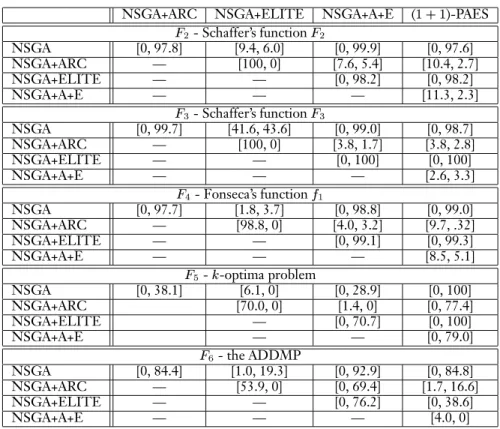
6- the ADDMP (1+1)-PAES [79.0, 0] [22.0, 0] [48.7, 0] [15.4, 0] [15.4, 0.5] 1+10 — [0, 0.2] [0, 0] [0, 0] [8.0, 75.3] 1+50 — — [4.3, 0] [0, 0] [0, 37.6] 10+1 — — — [0, 0] [0, 12.3] 10+10 — — — — [0, 3.0]

For reasons of clarity, we do not present the complete set of results described above. Nonetheless, only the tests carried out to decide on the best algorithm to carry forward to the ‘finals’ and the finals themselves are absent. All of the results for the internal tests for the Niched Pareto GA are presented in Table 6. Similar sets of results for the NSGA and the PAES algorithms can be found in Tables 8 and 7, respectively. The results of testing all algorithms against each other on their combined phenotype space are given in Table 9.

On

F

5, the

k

-optima problem, the results presented warrant further analysis and

discussion. To this end, plots of the best, worst, and median distributions over the phenotype range are included. These plots help to clarify the statistical data and also illustrate different methods of visualizing the performance of multiobjective optimizers.

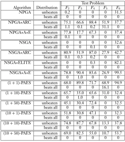
We find that the test described above in which all algorithms are tested against all others, in general, accurately reflects the results from the comparisons on pairs of algorithms on their own combined space. The percentage of the space on which an algorithm is unbeaten seems particularly reliable. For this reason, most of the following discussion is limited to the results presented in Table 9 only. A summary of these results is provided in Table 10.

6.2 (1+1)-PAES

Our original baseline approach, (1+1)-PAES, is the simplest and fastest of the methods

compared in this paper. Despite this, its performance on the test functions used here provides considerable evidence that it is a capable multiobjective optimizer on a range of problem types. In fact, among the thirteen algorithms tested here, it is perhaps the most reliable performer. When all algorithms are pair-wise compared against the combined nondominated front, (1+1)-PAES is unbeaten on, in the worst case, 68% of the front

(problem

F

2). On problem

F

5, (

1+1)-PAES covers the largest part of the Pareto front and

manages to find the most demanding solutions not generated by any of the other algorithms tested. (Problem

F

5is discussed further towards the end of the results section.) It seems

that (1+1)-PAES works well for the same reasons that it is computationally simple: it is an

aggressive algorithm, testing each solution generated in a stringent manner, and investing few resources in solutions which do not pass the test. In this sense, it is the analogue of a single-objective hillclimber. This has drawbacks, too. (1+1)-PAES (or 1+

) would be

stumped by any search space containing local optima that could not be traversed by its small change (mutation) operator, as it has no facility for moving from the current solution to an inferior one (in the Pareto sense). This is possibly less of a flaw in multiobjective spaces than in single objective ones because with more objectives the occurrence of functions with true local optima may be reduced. However, test function

F

3 is an example of a function

where a hillclimbing approach could get stuck. If an optimizer were to start in the right hand range of optima, i.e., with5

x >

4, it would not be able to move to the left optima

by small changes to the variable

x

. PAES does not suffer from this problem because

x

is encoded as an

n

-bit binary string, and PAES is allowed to move by changing one or more of the

n

bits. Therefore, it is able to jump across the divide.

Timings for six of the algorithms presented in this section are also included in Table 11. In this case, the test function (

F

5) takes only a small proportion of the total computation

time, so the differing computation times of each algorithm are clear. (1+1)-PAES is 37%

faster than its nearest rival, the NPGA, on this test problem.

6.3 (1+

)-PAES

The (1+10) and (1+50) variants of PAES do not do nearly as well as the baseline (1+1)

approach. Only on one problem,

F

4, does (1+50)-PAES generate better distributions over

the 20 runs than (1+1)-PAES, and (1+10)-PAES never does. The lack of competitiveness

of (1+

)-PAES might be explained with relation to its strategy for replacing the current solution. As in (1+1)-PAES, the current solution is first compared to each mutant. In

the case where exactly one member dominates the current solution, this will be accepted as the current solution of the next iteration. However, in all other cases, the acceptance is based upon the result of comparing each mutant with the archive of the previous iteration. Mutants are not compared one against the other. Any ties that occur are broken first with reference to the population in the mutants’ grid locations, and if this is inconclusive, randomly. This approach can lead to acceptance of a mutant that is dominated by one of the other mutants of its generation. In this case, some of the characteristic aggressiveness of (1+1)-PAES may be lost. The archive of the previous generation was used to balance the

need for a static test of the current generation with computational parsimony. Comparing mutants against a constantly updated archive may be preferable but requires a complicated process to ensure that the resultant ranking is correct. Rather than add extra complexity, the option of using the archive of the previous generation was taken. It is unclear at the

Table 8: Comparison of four variants of the Nondominated Sorting GA. NSGA+ARC NSGA+ELITE NSGA+A+E (1+1)-PAES

F

2- Schaffer’s function

F

2 NSGA [0, 97.8] [9.4, 6.0] [0, 99.9] [0, 97.6] NSGA+ARC — [100, 0] [7.6, 5.4] [10.4, 2.7] NSGA+ELITE — — [0, 98.2] [0, 98.2] NSGA+A+E — — — [11.3, 2.3]

F

3- Schaffer’s function

F

3 NSGA [0, 99.7] [41.6, 43.6] [0, 99.0] [0, 98.7] NSGA+ARC — [100, 0] [3.8, 1.7] [3.8, 2.8] NSGA+ELITE — — [0, 100] [0, 100] NSGA+A+E — — — [2.6, 3.3]

F

4- Fonseca’s function

f

1 NSGA [0, 97.7] [1.8, 3.7] [0, 98.8] [0, 99.0] NSGA+ARC — [98.8, 0] [4.0, 3.2] [9.7, .32] NSGA+ELITE — — [0, 99.1] [0, 99.3] NSGA+A+E — — — [8.5, 5.1]

F

5-

k

-optima problem NSGA [0, 38.1] [6.1, 0] [0, 28.9] [0, 100] NSGA+ARC [70.0, 0] [1.4, 0] [0, 77.4] NSGA+ELITE — [0, 70.7] [0, 100] NSGA+A+E — — [0, 79.0]

F

6- the ADDMP NSGA [0, 84.4] [1.0, 19.3] [0, 92.9] [0, 84.8] NSGA+ARC — [53.9, 0] [0, 69.4] [1.7, 16.6] NSGA+ELITE — — [0, 76.2] [0, 38.6] NSGA+A+E — — — [4.0, 0]

time of writing if this issue is, in fact, the only factor (or most important factor) affecting the performance of (1+

)-PAES, but this is under investigation.

6.4 (

+

)-PAES

The population-based variants, (10+1), (10+10), and (10+50) perform comparably with (1+ 1)-PAES on problems

F

2,

F

3, and

F

4. On

F

2, (10+10)-PAES is superior to (

1+1). However,

the population based methods do not fare well on

F

5or

F

6and lack the consistently high

performance of (1+1)-PAES. The use of a population does not, in general, improve the

performance of the basic PAES algorithm and adds considerable computational overhead (see Table 11). However, similar comments as those regarding the acceptance strategy used in (1+

)-PAES apply equally here to (

+

)-PAES.

6.5 The NPGAs

Turning now to the evolutionary algorithms, the first thing we notice is that, without ex-ception, the archived versions consistently outperform the nonarchived ones. Also, elitism is, generally, beneficial. The elitist technique employed in the NPGA is not so success-ful, however, only enhancing the results in one of the test problems and degrading them considerably in the others.

Table 9: Pair-wise comparisons of all algorithms on the combined phenotype space for all problems. Test Problem Algorithm Distribution

F

2

F

3

F

4

F

5

F

6 NPGA unbeaten 0.2 0 0 0 31.5 beats all 0 0 0 0 0 NPGA+ARC unbeaten 75.1 66.6 88.4 51.9 37.7 beats all 1.1 0.1 0.2 31.1 0 NPGA+A+E unbeaten 77.8 17.7 67.3 0 37.4 beats all 0.1 0 0 0 0 NSGA unbeaten 0 0 0 0 32.6 beats all 0 0 0.1 0 0 NSGA+ARC unbeaten 80.9 51.9 87.0 27.9 42.7 beats all 0.1 0.3 0.2 0 0 NSGA+ELITE unbeaten 0 0 0.3 0 82.1 beats all 0 0 0 0 0 NSGA+A+E unbeaten 78.8 90.4 83.6 26.9 99.5 beats all 0 1.0 0 0 0 (1+1)-PAES unbeaten 68.0 89.8 71.7 68.9 94.9 beats all 0 0 0 16.1 0 (1+10)-PAES unbeaten 65.7 35.0 65.6 31.0 32.4 beats all 0 1.0 0 0 0 (1+50)-PAES unbeaten 45.1 30.4 72.4 0 32.5 beats all 0 0 0 0 0 (10+1)-PAES unbeaten 51.8 30.8 47.1 0 32.3 beats all 0 0 0 0 0 (10+10)-PAES unbeaten 74.8 87.7 67.8 13.3 37.8 beats all 0 0 0 0 0 (10+50)-PAES unbeaten 69.0 82.5 55.0 10.7 53.7 beats all 0 0 0 0 0

Overall, the NPGA with archiving does quite well in comparison to both (1+1)-PAES

and the NSGA. It is superior to both of them on problem

F

4. On

F

6(the ADDMP), its

performance is weak, and it does not perform as consistently well as either the NSGA with archiving and elitism or our baseline approach (1+1)-PAES. It is also the most difficult

of the algorithms to use, requiring more parameters to be set, some of which can severely degrade performance if set incorrectly. Its computational complexity is low compared to either the population based PAES algorithms or the NSGAs because it does not have to explicitly assign fitness values to the population. However, (1+1)-PAES seems both a more

consistent performer (see Table 10) and a faster algorithm on the results presented here.

6.6 The NSGAs

The NSGAs recursively sort the current population into two sets, the nondominated and the dominated. This approach gives a fairly accurate estimate of the dominance rank of each individual, encouraging selection to focus on the best members of the population. This is perhaps why the NSGAs, when coupled with the archiving of all nondominated solutions and elitism perform slightly better than the NPGAs. It also employs a more accurate form

Table 10: Summary statistics for best 3 optimizers. NPGA+A NSGA+A+E (1+1)-PAES

F

2 rank 4 2 7 unbeaten 75.1 78.8 68.0

F

3 rank 5 1 2 unbeaten 66.6 90.4 89.8

F

4 rank 1 3 4 unbeaten 88.4 83.6 71.7

F

5 rank 2 5 1 unbeaten 51.9 26.9 68.9

F

6 rank 7 1 2 unbeaten 37.7 99.5 94.9 worst rank 7 5 7

overall sum of ranks 19 12 16

stats worst coverage 37.7 26.9 68.0 (unbeaten)

Table 11: Algorithm run times on test problem

F

5.

Run times on SPARC Ultra 10 300MHz Algorithm Mean (seconds) SD (seconds) (1+1)-PAES 1

:

85 0

:

0446 (10+50)-PAES 4

:

48 0

:

0283 NSGA 8

:

16 0

:

0988 NSGA+A+E 8

:

45 0

:

0127 NPGA 2

:

96 0

:

0853 NPGA+A+E 3

:

03 0

:

0729

of niching than the NPGA which approximates the niching process using equivalence class sharing.

The NSGA with archiving and elitism is ranked first on three of the five multiobjective test problems, when all algorithms are compared pair-wise on the overall combined space. Its lowest rank is on problem

F

5, where its performance is quite poor in comparison to

both the NPGA with archiving alone and those of some of the PAES algorithms. In fact, it is nondominated on only 26.9% of the combined space. These results are summarized in Table 10.

The NSGA is computationally expensive compared to either the NPGA or the local search versions of PAES. Its average time complexity is greater than either (see Section 2.4), requiring many comparisons to be made to rank the current population and to calculate the niche count so that fitness values can be assigned. When the NSGA was timed on test problem

F

5it was found to be the slowest algorithm here (see Table 11). Nonetheless, this

overhead is unimportant in many applications where the evaluation of solutions is by far the most time-consuming process in the search for solutions, and reducing the number of evaluations is more important.

0 0.2 0.4 0.6 0.8 1 0 0.2 0.4 0.6 0.8 1 NDSGA+ARC NPGA+ARC PAES(1+1) 0 0.2 0.4 0.6 0.8 1 0 0.2 0.4 0.6 0.8 1 NDSGA+ARC NPGA+ARC PAES(1+1) 0 0.2 0.4 0.6 0.8 1 0 0.2 0.4 0.6 0.8 1 NDSGA+ARC NPGA+ARC PAES(1+1) Worst Median Best

Figure 5: Best, median, and worst attainment surfaces found on

F

5.

6.7 Test Problem

F

5

From Table 9 it appears that the algorithm which is unbeaten on the largest percentage of the space does not always also beat all with the highest percentage. On

F

5(the

k

-optima

problem), for instance, (1+1)-PAES is unbeaten on 68.9% of the combined phenotype space

but only beats all on 16.1%. The NPGA with archiving, on the other hand, is unbeaten on less of the space but beats all on 31.1%. It would be interesting to see how these figures vary with the use of different confidence levels. In the case of problem

F

5, (

1+1)-PAES

beats all on 16% of the space because it has generated solutions at the edges of the range of optima where other algorithms have failed to do so. The NPGA, by contrast, has a better distribution in the center of the Pareto front.

For the time being, we indicate the difference in the distributions of points generated by the NPGA with archiving and (1+1)-PAES by plotting graphs of the best, worst, and

median attainment surfaces of these algorithms on problem

F

5. The best of the NSGAs

is also included in the graphs shown in Figure 54

. The NSGA is also interesting because although it appears to do relatively poorly from the statistical results, its best distribution is rather better than that of the NPGA. The best attainment surfaces show that (1+1)-PAES

finds optima that extend the furthest towards the ends of the Pareto front. The NSGA is nearly as good, and the NPGA is least impressive on this measure. This is why it is beaten on approximately 49% of the space. The median, similarly, is not favorable for the NPGA for the most part, although it beats the other two algorithms in a small portion of the space near the center. Finally, the plots of the worst attainment surface reveal why the

4

Note that all surfaces are orthogonal, although in the case of the median surfaces, this is only apparent at high resolution.

NPGA beats all the other algorithms on such a large percentage of the space. Its worst attainment surface, again in the center of the space, is significantly better than the other two algorithms. Returning to the comparison of pairs of algorithms on problem

F

5, it can be

seen that (1+1)-PAES had a better distribution than the NPGA with archiving on 48.2%

of the space compared to 34.7% vice versa. This result seems to be borne out by the plots in Figure 5 and gives, in this case, a truer picture of the algorithm with the best coverage of the space than the ‘beats all’ statistic discussed above.

7 Conclusion and Future Work

We have described PAES, which in its (1+1)-ES form can be viewed as a simple baseline

technique for multiobjective optimization. Some analysis of its time complexity has been provided, arguing that it requires fewer comparisons to perform selection and acceptance in the best case than two well-known and respected MOGAs. Timings of the algorithm on two problems provide empirical evidence to support this claim. It is a conceptually simple algorithm too, being the multiobjective analogue of a hillclimber.

Two extensions to the basic algorithm were also described, (1+

)-PAES and a population-based algorithm, (

+

)-PAES. All three algorithms exploit the same novel

means of evaluating solutions. An archive of nondominated solutions is kept, updated, and used as the benchmark by which newly generated solutions are judged. The archive also serves the purpose of recording nondominated solutions found for presentation at the end of the run. Parks and Miller (1998) employ an archive in a MOGA as a repository from which selection and breeding can occur. This use has not yet been investigated by the authors but is an interesting avenue for further work.

The main objective of the paper was to thoroughly test PAES on a range of test problems and to compare its performance with two well-known algorithms, the Niched Pareto Genetic Algorithm and a GA employing nondominated sorting. To achieve this, six test functions were used. Four of them have been used elsewhere as benchmarks for multiobjective optimizers, and two we introduced for the first time in this context. Six variants of PAES were tested against the NPGA and NSGA. Both genetic algorithms were modified to include versions that archived their solutions to allow them to store and present the nondominated solutions they had found. Elitist versions were also included. In all, thirteen algorithms were compared on the six test functions.

Statistical techniques introduced by Fonseca and Fleming (1995a) for the compari-son and assessment of multiobjective optimizers were employed in all our tests. These techniques allow univariate statistical analysis to be carried out on the attainment surfaces generated from several runs of a multiobjective optimizer. We thus found that PAES, par-ticularly in its baseline (1+1) form, is a capable multiobjective optimizer across a range

of problems. Its worst performance in terms of the percentage of the space on which it is unbeaten is superior to any of the other algorithms tested here. Where algorithms were ranked according to the percentage of the space on which they were unbeaten (see Table 10), (1+1)-PAES achieves the second lowest sum of ranks of the algorithms tested. On

this statistic, it is bettered only by the nondominated sorting GA employing both archiving and elitism. The two variants of PAES introduced in this paper did not fare as well on the test functions as the simpler baseline algorithm. A possible explanation for this is that the archive in these algorithms is not kept as strictly updated as in (1+1)-PAES so that some

There are various avenues for future work. An extension to PAES in which the archive is additionally used as a repository from which solutions can be selected might be a profitable line of research. Further investigation of the performance of (1+1)-PAES may also be

fruitful. As yet we are unsure how it moves about in the solution space and are intrigued to find out more about its performance, particularly on test problem

F

5 where it seems

to do particularly well. It may be important to measure the probability of obtaining an entire attainment surface with PAES because it is unclear from the statistics whether it can find solutions at both extremes of the optimal range on a single run. To do this may simply involve tracking it through a run, however, a more generally useful idea would be to extend the statistical technique of Fonseca and Fleming to allow such measures to be made. One way of doing this would be to acquire the worst, best, median, and interquartile range attainment surfaces in the normal way to use as benchmark surfaces in the solution space. Measurements from further runs could then be taken to ascertain the likelihood of an algorithm obtaining anentiresurface which covers each of these benchmark surfaces.

Acknowledgments

The authors are grateful to British Telecommunications Plc for financial support of the first author and to the anonymous reviewers for helpful and insightful comments.

References

B¨ack, T. (1996). Evolutionary Algorithms in Theory and Practice. Oxford University Press, Oxford, England.

Bentley, P. J. and Wakefield, J. P. (1997). Finding Acceptable Solutions in the Pareto-Optimal Range using Multiobjective Genetic Algorithms. In Chawdhry, P. K., Roy, R. and Pant, R. K., editors,

Soft Computing in Engineering and Design, Springer-Verlag, London, England.

Czyzak, P. and Jaszkiewicz, A. (1998). Pareto simulated annealing - a metaheuristic technique for multiple-objective combinatorial optimization.Journal of Multi-Criteria Decision Analysis, 7:34– 47.

Finkel, R. A. and Bentley, J. L. (1974). Quad trees: A data structure for retrieval on composite keys.

Acta Informatica, 4:1–9.

Fonseca, C. M. and Fleming, P. J. (1995a). An Overview of Evolutionary Algorithms in Multiobjective Optimization.Evolutionary Computation, 3(1):1–16.

Fonseca, C. M. and Fleming, P. J. (1995b). On the Performance Assessment and Comparison of Stochastic Multiobjective Optimizers. In Voigt, H.-M., Ebeling, W., Rechenberg, I. and Schwe-fel, H.-P., editors,Parallel Problem Solving From Nature IV, pages 584–593, Springer, Berlin, Germany.

Gandibleux, X., Mezdaoui, N. and Fr´eville, A. (1997). A tabu search procedure to solve multiobjective combinatorial optimization problems. Advances in Multiple Objective and Goal Programming -Lecture Notes in Economics and Mathematical Systems, 455:291–300.

Hansen, M. P. (1997). Tabu Search for Multiobjective Optimization : MOTS. In Stewart, T. and van den Honert, R., editors, Proceedings of the Thirteenth International Conference on Multiple Criteria Decision Making, Springer-Verlag, Berlin, Germany.

Hansen, M. P. (1998).Generating a Diversity of Good Solutions to a Practical Combinatorial Problem using Vectorized Simulated Annealing. Ph.D. thesis IMM-PHD-1998-45, Technical University of Denmark.