Exploratory spatial data analysis using Stata
Maurizio PisatiDepartment of Sociology and Social Research University of Milano-Bicocca (Italy)
2012 German Stata Users Group meeting WZB Social Science Research Center, Berlin
Outline
1 Introduction
2 Spatial data
3 Visualizing spatial data
Overview Dot maps
Proportional symbol maps Diagram maps
Choropleth maps Multivariate maps
Outline
4 Exploring spatial point patterns
Overview
Kernel density estimation
5 Detecting spatial autocorrelation
Overview
Spatial weights matrices
Measuring spatial autocorrelation Global indices of spatial autocorrelation Local indices of spatial autocorrelation
Exploratory spatial data analysis
• Exploratory spatial data analysis(Esda) is the
extension of exploratory data analysis (Eda) to the problem of detecting patterns in spatial data (Haining et al. 1998: 457)
• Esdainvolves seeking good descriptions of spatial data, so as to help the analyst to develop hypotheses and models for such data (Bailey and Gatrell 1995: 23)
• Esdaemphasizes graphical views of the data, designed to highlight meaningful clusters of observations, unusual observations, or relationships between variables. These views often take the form of maps
Esda
in Stata
• Stata users can perform Esdausing a variety of
user-written commands published in theStata Technical Bulletin, theStata Journal, or the SSC Archive
• In this talk, I will briefly illustrate the use of six such commands: spmap,spgrid,spkde,spatwmat,spatgsa,
Esda
in Stata
• spmap is a general command aimed at visualizing several
kinds of spatial data
• spgridgenerates two-dimensional grids covering
rectangular or irregular study areas
• spkde implements a variety of nonparametric kernel-based
estimators of the probability density function and the intensity function of two-dimensional spatial point patterns
• spatwmatimports or generates several kinds of spatial
weights matrices
• spatgsa computes global indices of spatial autocorrelation
Spatial data: a discrete view
• For simplicity, let us represent spaceas a plane, i.e., as a flat two-dimensional surface
• In spatial data analysis, we can distinguish two conceptions of space (Bailey and Gatrell 1995: 18):
• Entity view: Space as an area filled with a set of discrete
objects
• Field view: Space as an area covered with essentially
continuous surfaces
• Here we take the former view and define spatial data as information regarding a given set of discrete spatial objects located within a study areaA
Attributes of spatial objects
• Information about spatial objects can be classified into two categories:
• Spatial attributes
• Non-spatial attributes
• The spatial attributes of a spatial object consist of one
or more pairs of coordinates that represent its shape and/or its location within the study area
• The non-spatial attributesof a spatial object consist of
its additional features that are relevant to the analysis at hand
Types of spatial objects
• According to their spatial attributes, spatial objectscan be classified into several types
• Here, we focus on two basic types:
• Points (point data)
Points
• A point si is a zero-dimensional spatial object located within study area A at coordinates (si1, si2)
• Points can represent several kinds of real entities, e.g., dwellings, buildings, places where specific events took place, pollution sources, trees
Washington D.C. (2009)
Polygons
• A polygon ri is aregion of study area Abounded by a closed
polygonal chain whoseM ≥4
vertices are defined by the coordinate set{(ri1(1), ri2(1)), (ri1(2), ri2(2)), . . . ,(ri1(m), ri2(m)), . . . ,(ri1(M), ri2(M))}, where ri1(1)=ri1(M) and ri2(1)=ri2(M)
• Polygons can represent several kinds of real entities, e.g., states, provinces, counties, census tracts, electoral districts, parks, lakes
First Sixth Fourth Fifth Seventh Second Third Washington D.C. Police Districts
Mapping
• Most exploratory analyses of spatial data have their natural starting point in displaying the information of
interest by one or more maps
• If properly designed, maps can help the analyst to detect interesting patterns in the data, spatial relationships between two or more phenomena, unusual observations, and so on
Thematic maps
• In this talk I consider only the kind of maps most useful to
Esda: thematic maps
• Thematic maps represent the spatial distribution of a
phenomenon of interest within a given study area (Slocum
Thematic maps in Stata
• Stata users can generate thematic maps using spmap, a user-written command freely available from the SSC Archive (latest version: 1.2.0)
• spmap is a very flexible command that allows for creating a
large variety of thematic maps, from the simplest to the most complex
• While providing sensible defaults for most options and supoptions,spmap gives the user full control over the formatting of almost every map element, thus allowing the production of highly customized maps
Thematic maps in Stata
• In the following, I will show how to use spmapfor creating
the types of thematic maps most commonly used inEsda:
• Dot maps
• Proportional symbol maps
• Diagram maps
• Choropleth maps
Dot maps
• A dot mapshows the spatial distribution of a set of point
spatial objects S≡ {si;i= 1, . . . , N}, i.e., their location within a given study area A
• If the point spatial objects have variable attributes, it is possible to represent this information using symbols of different colors and/or of different shape
Dot maps: example 1
Spatial distribution of 359 cases of sex abuse, Washington D.C. (2009) !"#$%&'()#*++,-./0%!$12#0'$ 3#4#'0/#$567$"$#$$ "8)08$!"(43$%9:!4.0'(#"-./0%!$(.%567&$;1:2:'%#33"<#22&$$$$$$'''$ $$$8:(4/%=%=51::'.&$>%>51::'.&$"#2#1/%?##8$(;$:;;#4"#""(&$$$'''$ $$$$$"(@#%)*+,&$;1:2:'%'#.&$:1:2:'%A<(/#&$:"(@#%)-+.&&$$$$$$'''$ $$$/(/2#%%B#=$0C!"#"%!$"(@#%)*+,&&$$$$$$$$$$$$$$$$$$$$$$$$$$'''$ $$$"!C/(/2#%%D0"<(43/:4$7-&-$E*++,F%$%$%!$"(@#%)*+,&&! Washington D.C. (2009) Sex abuses
Dot maps: example 2
Spatial distribution of 359 cases of sex abuse, Washington D.C. (2009). Different colors are used to distinguish adult victims from child victims
!"#$%&'()#*++,-./0%!$12#0'$ 3#4#'0/#$567$"$#$$ 3#4#'0/#$8(1/()$"$)#/9:.$ '#1:.#$8(1/()$%&'(")*%)(')+",*%-".*$ 20;#2$.#<(4#$8(1/()$)$%=.!2/%$,$%&9(2.%$ 20;#2$802!#"$8(1/()$8(1/()$ ">)0>$!"(43$%?:!4.0'(#"-./0%!$(.%567*$<1:2:'%#33"9#22*$$$$$$'''$ $$$>:(4/%@%@51::'.*$A%A51::'.*$"#2#1/%B##>$(<$:<<#4"#""/*$$$'''$ $$$$$;A%8(1/()*$"(C#%-).,*$<1:2:'%'#.$408A*$$$$$$$$$$$$$$$$$'''$ $$$$$:1:2:'%D9(/#$..*$:"(C#%-0.1$..*$2#3#4.0%:4*$$$$$$$$$$$$'''$ $$$$$2#31:!4/*$$$$$$$$$$$$$$$$$$$$$$$$$$$$$$$$$$$$$$$$$$$$$$'''$ $$$2#3#4.%"(C#%-).+*$':D30>%).,**$$$$$$$$$$$$$$$$$$$$$$$$$$$'''$ $$$/(/2#%%E#@$0;!"#"F$;A$8(1/()$03#%!$"(C#%-).,**$$$$$$$$$$$'''$ $$$"!;/(/2#%%G0"9(43/:4$7-&-$H*++,I%$%$%!$"(C#%-).,**! Adult (155) Washington D.C. (2009)
Dot maps: example 3
Spatial distribution of 359 cases of sex abuse, Washington D.C. (2009). Major roads, watercourses and parks are added to the map for reference
!"#$%&'()#*++,-./0%!$12#0'$ 3#4#'0/#$567$"$#$$ "8)08$!"(43$%9:!4.0'(#"-./0%!$(.%567&$;1:2:'%#33"<#22&$$$$$$'''$ $$$8:(4/%=%=51::'.&$>%>51::'.&$"#2#1/%?##8$(;$:;;#4"#""(&$$$'''$ $$$$$"(@#%)*+,&$;1:2:'%'#.&$:1:2:'%A<(/#&$:"(@#%)-+.&&$$$$$$'''$ $$$8:2>3:4%.0/0%%B0/#'CD0'?"-./0%&$E>%/>8#&$$$$$$$$$$$$$$$$$'''$ $$$$$:1:2:'%4:4#$++&$;1:2:'%3'##4$E2!#&&$$$$$$$$$$$$$$$$$$$$'''$ $$$2(4#%.0/0%%F0G:'H:0."-./0%&$1:2:'%E':A4&&$$$$$$$$$$$$$$$$'''$ $$$/(/2#%%I#=$0E!"#"%!$"(@#%)*+,&&$$$$$$$$$$$$$$$$$$$$$$$$$$'''$ $$$"!E/(/2#%%B0"<(43/:4$7-&-$J*++,K%$%$%!$"(@#%)*+,&&! Washington D.C. (2009) Sex abuses
Proportional symbol maps
• A proportional symbol map represents the values taken
by a numeric variable of interest Y on a set of point spatial objectsS located within a given study area A
• Proportional symbol maps can be used with two types of point data (Slocumet al. 2005: 310):
• True point dataare measured at actual point locations
• Conceptual point dataare collected over a set of regions
R≡ {ri;i= 1, . . . , N}, but are conceived as being located
at representative points within the regions, typically at their centroids
• The area of each point symbol is sized in direct proportion to the corresponding value of Y
Proportional symbol maps: example 1
Mean family income in the seven Police Districts of Washington D.C. (2000) !"#$%&'()*#+)",-)*,".+/,/01,/%!$*(#/-$ 2#3#-/,#$4$"$)3*'5#65/#$%%%$ 7'-5/,$4$&'($7$ "85/8$!")32$%&'()*#+)",-)*,".9''-1)3/,#"01,/%!$)1))1*$$$$$$$###$ $$$7*'('-)#22":#((*$$$$$$$$$$$$$$$$$$$$$$$$$$$$$$$$$$$$$$$$$###$ $$$8')3,););6*''-1*$<)<6*''-1*$8-'8'-,)'3/()4*$7*'('-)-#1*$$###$ $$$$$'*'('-)=:),#*$")>#)+,(-**$$$$$$$$$$$$$$$$$$$$$$$$$$$$$$###$ $$$(/?#(););6*''-1*$<*''-1)<6*''-1*$(/?#()4*$*'('-)=:),#*$$$###$ $$$$$")>#)+$('**$$$$$$$$$$$$$$$$$$$$$$$$$$$$$$$$$$$$$$$$$$$$###$ $$$,),(#)%@#/3$7/5)(<$)3*'5#$A)3$,:'!"/31"$'7$BC$1'((/-"D%*$###$ $$$"!?,),(#)%E/":)32,'3$+090$AFGGGD%$%$%*! 26.1 12.7 19.6 14.0 8.1 51.5 22.7 Washington D.C. (2000)
Proportional symbol maps: example 2
Mean family income in the 188 Census Tracts of Washington D.C. (2000). Solid circles denotepositive deviations from the overall mean income, hollow circles denotenegative deviations. Circles are drawn with size proportional to the absolute value of the deviation
!"#$%&#'"!"()))*+,-,./-,%!$01#,2$ 3#'#2,-#$4$"$5'067#87,#$%%%$
"97,9$!"5'3$%&#'"!"()))*&662/5',-#"./-,%!$5/&5/'$$$$$$$$$$$###$ $$$:06162!";#11'$$$$$$$$$$$$$$$$$$$$$$$$$$$$$$$$$$$$$$$$###$ $$$965'-&<&<80662/'$=&=80662/'$:06162&2#/'$606162&>;5-#'$$$###$ $$$$$"5?#&(%)*'$/#@5,-56'&4'$2#:>#53;-&969-6-''$$$$$$$$$$$$###$ $$$-5-1#&%A#,'$:,751=$5'067#%'$$$$$$$$$$$$$$$$$$$$$$$$$$$$$###$ $$$"!B-5-1#&%C,";5'3-6'$+.&.$D()))E%$%$%'!
Washington D.C. (2000)
Diagram maps
• A diagram map follows the same logic as a proportional
symbol map, but represents the values of the variable of interest using bar charts, pie charts, or other types of diagram
• The use of pie charts allows to display the spatial distribution of compositional data, i.e., of two or more numeric variables that represent parts of a whole
Diagram maps: example 1
Mean family income in the seven Police Districts of Washington D.C. (2000). Data are represented by framed-rectangle charts, with the overall mean income as the reference value
!"#$%&'()*#+)",-)*,".+/,/01,/%!$*(#/-$ "23/2$!")45$%&'()*#+)",-)*,".6''-1)4/,#"01,/%!$)1")1#$$$$$$$$$$$ $$$7*'('-"#55"8#((#$$$$$$$$$$$$$$$$$$$$$$$$$$$$$$$$$$$$$$$$$$$$$ $$$1)/5-/3"9/-")4*'3#:3/#$-#7;#)58,"2'2,',#$7*'('-"5-##4#$$$$$$$ $$$$$$<"<:*''-1#$="=:*''-1#$")>#"%&'##$$$$$$$$$$$$$$$$$$$$$$$$$$ $$$,),(#"%?#/4$7/3)(=$)4*'3#%#$$$$$$$$$$$$$$$$$$$$$$$$$$$$$$$$$$ $$$"!@,),(#"%A/"8)45,'4$+060$BCDDDE%$%$%#! Washington D.C. (2000) Mean family income
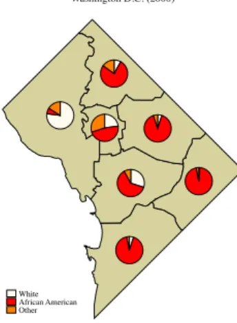
Diagram maps: example 2
Race/Ethnic composition of the
population of the seven Police Districts of Washington D.C. (2000). Data are represented by pie charts
!"#$%&'()*#+)",-)*,".+/,/01,/%!$*(#/-$ 2#3#-/,#$45),#67*,$"$7'7645),##7'7,',$%&&$ 2#3#-/,#$/8-'/967*,$"$7'76/8-'/9#7'7,',$%&&$ 2#3#-/,#$',5#-67*,$"$7'76',5#-#7'7,',$%&&$ (/:#($;/-)/:(#$45),#67*,$%<5),#%$ (/:#($;/-)/:(#$/8-'/967*,$%=8-)*/3$=9#-)*/3%$ (/:#($;/-)/:(#$',5#-67*,$%>,5#-%$ "79/7$!")32$%&'()*#+)",-)*,".?''-1)3/,#"01,/%!$)1')1($$$$$$$###$ $$$8*'('-'",'3#($$$$$$$$$$$$$$$$$$$$$$$$$$$$$$$$$$$$$$$$$$$$###$ $$$1)/2-/9';/-'45),#67*,$/8-'/967*,$',5#-67*,($@'@6*''-1($$$###$ $$$$$A'A6*''-1($8*'('-'#22"5#(($-#1$'-/32#($")B#'%)*($$$$$$$###$ $$$$$(#2#31/''3(($$$$$$$$$$$$$$$$$$$$$$$$$$$$$$$$$$$$$$$$$$$###$ $$$(#2#31'")B#'$%)+(($$$$$$$$$$$$$$$$$$$$$$$$$$$$$$$$$$$$$$$###$ $$$,),(#'%C/*#DE,53)*$*'97'"),)'3$'8$,5#$7'7!(/,)'3%($$$$$$$###$ $$$"!:,),(#'%</"5)32,'3$+0?0$FGHHHI%$%$%(! Washington D.C. (2000)
Choropleth maps
• A choropleth map displays the values taken by a variable
of interest Y on a set of regionsR within a given study
area A
• When Y is numeric, each region is colored or shaded according to a discrete scale based on its value on Y
• The number of classes k that make up the discrete scale, and the corresponding class breaks, can be based on several different criteria – e.g., quantiles, equal intervals, boxplot, standard deviates
Choropleth maps: example 1
Mean family income in the 188 Census Tracts of Washington D.C. (2000). Income is divided into six classes based on thequantiles method
!"#$%&#'"!"()))*+,-,./-,%!$01#,2$ 3#'#2,-#$4$"$5'067#87,#$%%%$ 9627,-$4$&'(%9$ ":7,:$4$!"5'3$%&#'"!"()))*&662/5',-#"./-,%!$5/)5/*$$$$$$$$$$###$ $$$01'!7;#2)+*$017#-<6/)=!,'-51#*$906162)>!?/*$$$$$$$$$$$$$$###$ $$$'/906162)3"@*$'/1,;)%A5""5'3%*$$$$$$$$$$$$$$$$$$$$$$$$$$$###$ $$$1#3#'/)"5B#),$(-**$$$$$$$$$$$$$$$$$$$$$$$$$$$$$$$$$$$$$$$###$ $$$-5-1#)%A#,'$9,751C$5'067#$D5'$-<6!",'/"$69$EF$/611,2"G%*$###$ $$$"!;-5-1#)%H,"<5'3-6'$+.&.$D()))G%$%$%*! (93,341] (54,93] (40,54] Washington D.C. (2000)
Choropleth maps: example 2
Mean family income in the 188 Census Tracts of Washington D.C. (2000). Income is divided into six classes based on theequal intervals method
!"#$%&#'"!"()))*+,-,./-,%!$01#,2$ 3#'#2,-#$4$"$5'067#87,#$%%%$ 9627,-$4$&'(%9$ ":7,:$4$!"5'3$%&#'"!"()))*&662/5',-#"./-,%!$5/)5/*$$$$$$$$$$###$ $$$01'!7;#2)+*$017#-<6/)#=5'-*$906162)>!?/*$$$$$$$$$$$$$$$$$###$ $$$'/906162)3"@*$'/1,;)%A5""5'3%*$$$$$$$$$$$$$$$$$$$$$$$$$$$###$ $$$1#3#'/)"5B#),$(-**$$$$$$$$$$$$$$$$$$$$$$$$$$$$$$$$$$$$$$$###$ $$$-5-1#)%A#,'$9,751C$5'067#$D5'$-<6!",'/"$69$EF$/611,2"G%*$###$ $$$"!;-5-1#)%H,"<5'3-6'$+.&.$D()))G%$%$%*! (285,341] (230,285] (174,230] (118,174] (62,118] [6,62] Washington D.C. (2000)
Choropleth maps: example 3
Mean family income in the 188 Census Tracts of Washington D.C. (2000). Income is divided into six classes based on theboxplot method
!"#$%&#'"!"()))*+,-,./-,%!$01#,2$ 3#'#2,-#$4$"$5'067#87,#$%%%$ 9627,-$4$&'(%9$ ":7,:$4$!"5'3$%&#'"!"()))*&662/5',-#"./-,%!$5/)5/*$$$$$$$$$$###$ $$$01'!7;#2)+*$017#-<6/);6=:16-*$906162)>!?/*$$$$$$$$$$$$$$$###$ $$$'/906162)3"@*$'/1,;)%A5""5'3%*$$$$$$$$$$$$$$$$$$$$$$$$$$$###$ $$$1#3#'/)"5B#),$(-**$$$$$$$$$$$$$$$$$$$$$$$$$$$$$$$$$$$$$$$###$ $$$-5-1#)%A#,'$9,751C$5'067#$D5'$-<6!",'/"$69$EF$/611,2"G%*$###$ $$$"!;-5-1#)%H,"<5'3-6'$+.&.$D()))G%$%$%*! (132,341] (71,132] (40,71] Washington D.C. (2000)
Choropleth maps: example 4
Mean family income in the 188 Census Tracts of Washington D.C. (2000). Income is divided into four classes based on thestandard deviates method
!"#$%&#'"!"()))*+,-,./-,%!$01#,2$ 3#'#2,-#$4$"$5'067#87,#$%%%$ 9627,-$4$&'(%9$ ":7,:$4$!"5'3$%&#'"!"()))*&662/5',-#"./-,%!$5/)5/*$$$$$$$$$$###$ $$$01'!7;#2)+*$017#-<6/)"-/#=*$906162)>!?/*$$$$$$$$$$$$$$$$$###$ $$$'/906162)3"@*$'/1,;)%A5""5'3%*$$$$$$$$$$$$$$$$$$$$$$$$$$$###$ $$$1#3#'/)"5B#),$(+**$$$$$$$$$$$$$$$$$$$$$$$$$$$$$$$$$$$$$$$###$ $$$-5-1#)%A#,'$9,751C$5'067#$D5'$-<6!",'/"$69$EF$/611,2"G%*$###$ $$$"!;-5-1#)%H,"<5'3-6'$+.&.$D()))G%$%$%*! (110,341] (59,110] (9,59] [6,9] Washington D.C. (2000)
Multivariate maps
• A multivariate mapcombines several types of thematic
mapping to simultaneously display the spatial distribution of multiple phenomena within a given study area A
Multivariate maps: example 1
The map shows the relationship between mean family income (represented by framed-rectangle charts) and pct. white population (represented by shades of color) across the seven Police Districts of Washington D.C. (2000)
!"#$%&'()*#+)",-)*,".+/,/01,/%!$*(#/-$
2#3#-/,#$4$"$5'5678),##5'5,',$%&&$
9'-:/,$4$'()&9$
"5:/5$4$!")32$%&'()*#+)",-)*,".;''-1)3/,#"01,/%!$)1*)1+$$$$$###$ $$$*(:#,8'1**!",':+$*(<-#/="*&$(,$,&$-,$%&&+$9*'('-*4(>3+$$$###$ $$$(#2,),*%&*,0$78),#$5'5!(/,)'3%+$$$$$$$$$$$$$$$$$$$$$$$$$$###$ $$$1)/2-/:*?/-*)3*':#6:/+$-#97#)28,*5'5,',+$9*'('-*-#1+$$$$$###$ $$$$$@*@6*''-1+$A*A6*''-1+$")B#*%).++$$$$$$$$$$$$$$$$$$$$$$$###$ $$$(#2#31*")B#*$%)/++$$$$$$$$$$$$$$$$$$$$$$$$$$$$$$$$$$$$$$$###$ $$$,),(#*%C#/3$9/:)(A$)3*':#$/31$5*,0$78),#$5'5!(/,)'3%+$$$$###$
$$$"!<,),(#*%D/"8)32,'3$+0;0$EFGGGH%$%$%+! Pct. white population (75,100] (50,75] (25,50]
Washington D.C. (2000)
Multivariate maps: example 2
The map shows the relationship between pct. white population (represented by framed-rectangle charts), mean family income (represented by the width of framed-rectangle charts) and robbery rate (represented by shades of color) across the seven Police Districts of Washington D.C. (2000/2009)!"#$%&'()*#+)",-)*,".+/,/01,/%!$*(#/-$
2#3#-/,#$4$"$5'5678),##5'5,',$%&&$
9'-:/,$4$'()&9$
"5:/5$4$!")32$%&'()*#+)",-)*,".;''-1)3/,#"01,/%!$)1*)1+$$$$$###$ $$$*(:#,8'1**!",':+$*(<-#/="*&$(,$,&$-,$%&&+$9*'('-*4(>3+$$$###$ $$$(#2,),*%&*,0$78),#$5'5!(/,)'3%+$$$$$$$$$$$$$$$$$$$$$$$$$$###$ $$$1)/2-/:*?/-*)3*':#6:/+$-#97#)28,*5'5,',+$9*'('-*-#1+$$$$$###$ $$$$$@*@6*''-1+$A*A6*''-1+$")B#*%).++$$$$$$$$$$$$$$$$$$$$$$$###$
$$$(#2#31*")B#*$%)/++$$$$$$$$$$$$$$$$$$$$$$$$$$$$$$$$$$$$$$$###$ Robberies per 1,000 pop.
Washington D.C. (2000/2009) Pct. white population, income and robberies
Two-dimensional spatial point patterns
• A two-dimensional spatial point patterncan be
defined as a set of N point spatial objectsS located within a given study area A
• Usually, each point si∈S represents a real entity of some kind: people, events, sites, buildings, plants, cases of a disease, etc.
• Alternatively, each point si represents the centroid of a region
Two-dimensional spatial point patterns
• In the analysis of spatial point patterns, we are often interested in determining whether the observed data points exhibit some form of clustering, as opposed to being
distributed uniformly within A
• To explore the possibility of point clustering, it may be useful to describe the spatial point pattern of interest by means of its probability density function p(s) and/or its intensity functionλ(s) (Waller and Gotway 2004)
Two-dimensional spatial point patterns
• The probability density functionp(s) defines the
probability of observing an object per unit area at location
s∈ A
• The intensity functionλ(s) defines the expected number
of objects per unit area at location s∈ A
• The probability density function and the intensity function differ only by a constant of proportionality
Kernel estimators
• Both the probability density functionp(s) and the intensity functionλ(s) of a two-dimensional spatial point pattern can be estimated by means of nonparametric estimators, e.g., kernel estimators (Waller and Gotway 2004)
• Kernel estimators are used to generate a spatially
smooth estimate ofp(s) and/or λ(s) at a fine grid of points
sg (g= 1, ..., G) covering the study area A
• In the context of spatial data analysis, a gridis a regular tessellation of the study areaA that divides it into a set of G contiguous cells whose centers are referred to as thegrid points and denoted by sg
Kernel estimator of
λ
(
s
)
• The intensity λ(sg) at each grid pointsg is estimated by: ˆ λ(sg) = c Ag N X i=1 k d(si,sg) hi yi
where k(·) is thekernel function – usually a unimodal symmetrical bivariate probability density function;hi is the
kernel bandwidth, i.e., the radius of the kernel function; d(si,sg) is the Euclidean distance between data pointsi and grid pointsg;yi is the value taken by an optional variable of interest Y at data pointsi;Ag is the area of the region of A over which the kernel function is evaluated, possibly corrected for edge effects; and cis a constant of
Kernel estimator of
p
(
s
)
• In turn, the probability density p(sg) at each grid pointsg is estimated by: ˆ p(sg) = ˆ λ(sg) G P j=1 ˆ λ(sj)
Kernel estimation in Stata
• Stata users can generate kernel estimates of the probability density function p(s) and the intensity function λ(s) using two user-written commands freely available from the SSC
Archive: spgridandspkde
• spgrid(latest version: 1.0.1) generates several kinds of
two-dimensional grids covering rectangular or irregular study areas
• spkde (latest version: 1.0.0) implements a variety of kernel
estimators of p(s) and λ(s)
• spmap can then be used to visualize the kernel estimates
Kernel estimation: example
Our purpose is to estimate the probability density function of a set of 139 points representing thehomicidescommitted in Washington D.C. in 2009
Kernel estimation: example
Step 1
We usespgridto generate a grid covering the area of Washington D.C. We choose a relatively fine grid resolution (grid cell width = 200 meters). spmapis used to display the grid
!"#$%&'(!%)#'*+,()&-$%.!/&0-*!'$.!,1(0%,)"2344#''''$$$' '''&,0!'5,6"$.!!'()%0"6.0.$!#'5.11!"*50.6"/&0-*#'''$$$' '''",%)0!"*"0.6"/&0-*#'$."1-5.' ' (!.'*"0.6"/&0-*!'51.-$' !"6-"'(!%)#'*50.6"/&0-*!'%&"!"#$%&7%&#!
Kernel estimation: example
Step 2
We usespkdeto generate kernel estimates of the probability distribution of homicides in Washington D.C. We choose a quartic kernel function with fixed bandwidth equal to 1,000 meters and edge correction. spmapis used to display the results
!"#$%&'()#*++,-./0%!$12#0'$ 3##4$(5$655#7"#""#$ "43.#$!"(78$%4/#)4-./0%!$9$9:166'.%$;$;:166'.%$$$&&&$ $$$3#'7#2$<!0'/(1%$=07.>(./?$5=>%$5=>$'(((%$$$$$$&&&$ $$$#.8#16''#1/$.6/"$"0@(78$%3.#-./0%!$'#4201#%$ $ !"#$%3.#-./0%!$12#0'$ "4)04$4$!"(78$%1/#)4-./0%!$(.$"48'(.:(.%$12)#/?6.$<!07/(2#%$&&&$ $$$127!)=#'$)(%$51626'$A0(7=6>%$61626'$767#$**%$2#8#7.$655%$&&&$ $$$/(/2#$%B6)(1(.#"%!$"(C#$+'*)%%$$$$$$$$$$$$$$$$$$$$$$$$$$$&&&$ $$$"!=/(/2#$%D0"?(78/67$E-&-$F*++,G%$%$%!$"(C#$+'*)%%! Washington D.C. (2009) Homicides
Kernel estimation: example
Step 2
We usespkdeto generate kernel estimates of the probability distribution of homicides in Washington D.C. We choose a quartic kernel function with fixed bandwidth equal to 1,000 meters and edge correction. spmapis used to display the results
!"#$%&'()#*++,-./0%!$12#0'$ 3##4$(5$655#7"#""#$ "43.#$!"(78$%4/#)4-./0%!$9$9:166'.%$;$;:166'.%$$$&&&$ $$$3#'7#2$<!0'/(1%$=07.>(./?$5=>%$5=>$'(((%$$$$$$&&&$ $$$#.8#16''#1/$.6/"$"0@(78$%3.#-./0%!$'#4201#%$ $ !"#$%3.#-./0%!$12#0'$ "4)04$4$!"(78$%1/#)4-./0%!$(.$"48'(.:(.%$12)#/?6.$<!07/(2#%$&&&$ $$$127!)=#'$)(%$51626'$A0(7=6>%$61626'$767#$**%$2#8#7.$655%$&&&$ Washington D.C. (2009) Homicides
Spatial autocorrelation
• Forty years ago, the geographer and statistician Waldo Tobler formulated the first law of geography: “Everything is related to everything else, but near things are more related than distant things” (Tobler 1970: 234)
• This “law” defines the statistical concept of (positive)
spatial autocorrelation, according to which two or more
objects that are spatially close tend to be more similar to each other – with respect to a given attributeY – than are spatially distant objects
• In general, spatial autocorrelation impliesspatial
custering, i.e., the existence of sub-areas of the study area
Spatial weights matrix
• The analysis of spatial autocorrelation requires the
measurement of the degree of spatial proximityamong
the spatial objects of interest
• Typically, the degree of spatial proximity among a given set ofN spatial objects is represented by aN ×N matrix
called spatial weights matrixand denoted byW
• Each element (i, j) of W – which we denote bywij – expresses the degree of spatial proximity between the pair of objects iand j
• Depending on the application, theN main diagonal
Spatial weights matrix
• A common variant of Wis therow-standardized spatial
weights matrix Wstd, whose elements are defined as
follows: wstdij = wij N P j=1 wij
Spatial weights matrices in Stata
• Stata users can generate several kinds of spatial weights
matrices using spatwmat, a user-written command
published in theStata Technical Bulletin (Pisati 2001)
• spatwmat(latest version: 1.0) imports or generates from
scratch the spatial weights matrices required by the
Indices of spatial autocorrelation
• We consider measures of spatial autocorrelation that apply toarea data
• Measures of spatial autocorrelation can be classified into two broad categories:
• Global indices of spatial autocorrelation
Global indices of spatial autocorrelation
• A global index of spatial autocorrelation expresses
the overall degree of similarity between spatially close regions observed in a given study areaA with respect to a numeric variable Y (Pfeifferet al. 2008)
• Since global indices of spatial autocorrelation summarize the phenomenon of interest in a single value, they are intended not so much for identifying specific spatial
clusters, as for detecting the presence of a general tendency to clustering within the study area
Global indices of spatial autocorrelation
• In general, the computation of a global index of spatial autocorrelation follows a three-step procedure:
• First, we compute the degree of similarityρij between every
possible pair or regionsri andrj with respect to the
numeric variable of interestY
• Second, we weight – i.e., multiply – each valueρij by the
degree of proximitywij between regionsri andrj
• Finally, we sum up all the productswijρij and divide the
total by a constant of proportionality
• The greater the number of regions that are similar with respect toY and spatially close, the greater the value taken by the global index of spatial autocorrelation
Moran’s
I
• Moran’s global index of spatial autocorrelationI (Moran
1948) defines ρij as (yi−y¯)(yj−y¯), where yi is the value taken by Y in regionri,yj is the value taken byY in regionrj, and ¯y is the average value ofY:
I = N P i=1 N P j=1 wij(yi−y¯)(yj−y¯) 1 N N P i=1 (yi−y¯)2 N P i=1 N P j=1 wij where wii= 0
Moran’s
I
• Under the null hypothesis of no global spatial auto-correlation, the expected value of I is:
E(I) =− 1
N −1
• I > E(I) indicatespositive spatial autocorrelation –
nearby regions tend to exhibit similar values of Y
• I < E(I) indicatesnegative spatial autocorrelation –
Getis and Ord’s
G
• Getis and Ord’s global index of spatial autocorrelation G
(Getis and Ord 1992) definesρij asyiyj:
G= N P i=1 N P j=1 wijyiyj N P i=1 N P j=1 yiyj (i6=j)
where wij denotes the elements of a non-standardized binary spatial weights matrix, with wii= 0
Getis and Ord’s
G
• Under the null hypothesis of no global spatial auto-correlation, the expected value of Gis:
E(G) = N P i=1 N P j=1 wij N(N−1)
• G > E(G) indicates (a) positive spatial autocorrelation,
and (b) prevalence of spatial clusters with relatively high values of Y
• G < E(G) indicates (a) positive spatial autocorrelation,
Global indices of spatial autocorrelation in Stata
• Stata users can compute global indices of spatial auto-correlation using spatgsa, a user-written command published in theStata Technical Bulletin (Pisati 2001)
• spatgsa (latest version: 1.0) computes three global indices
of spatial autocorrelation: Moran’s I, Getis and Ord’sG, and Geary’s c. For each index and each numeric variable of interest, spatgsacomputes and displays in tabular form the value of the index itself, the expected value of the index under the null hypothesis of no global spatial
auto-correlation, the standard deviation of the index, the
Global indices of spatial autocorrelation: example
• Study area: Ohio
• Regions: 88 counties
• Variables of interest:
• Pct. population aged 18+ with poor-to-fair health status
(pct poorhealth)
• Pct. population aged 18+ currently smoking
(pct currsmoker)
• Pct. population aged 18+ ever diagnosed with high blood
pressure (pct hibloodprs)
Global indices of spatial autocorrelation: example
Step 1
We usespatwmatto import an existing binary spatial weights matrix
– stored in the Stata datasetCounties-Contiguity.dta – and
convert it into a properly formatted row-standardized spatial weights
matrixWs
!"#$%&#$'(!)*+',-.(*$)/!0-.*$)+()$123$#,!'''"""' '''*#&/#4!$'!$#*3#53)6/!
Global indices of spatial autocorrelation: example
User: Maurizio
The following matrix has been created:
1. Imported binary weights matrix Ws (row-standardized)
Dimension: 88x88
Global indices of spatial autocorrelation: example
Step 2
We usespatgsawith the spatial weights matrixWsto compute
Moran’sI on the variables of interest
!"#$%&'!()*#"+,-)-./)-%!$01#-2$
"3-)4"-$30)53''26#-1)6$30)50!22"7'8#2$30)56*91''/32"$$$"""$
Global indices of spatial autocorrelation: example
User: MaurizioMeasures of global spatial autocorrelation
Weights matrix Name: Ws
Type: Imported (binary) Row-standardized: Yes
Moran's I
Variables I E(I) sd(I) z p-value* pct_poorhealth 0.399 -0.011 0.065 6.337 0.000 pct_currsmoker 0.339 -0.011 0.065 5.367 0.000 pct_hibloodprs 0.126 -0.011 0.065 2.119 0.017 pct_obese 0.167 -0.011 0.065 2.730 0.003 *1-tail test
Global indices of spatial autocorrelation: example
Step 3
We use againspatwmatto import the binary spatial weights matrix
stored in the Stata datasetCounties-Contiguity.dta. This time,
however, we convert it into a properly formatted non-standardized
spatial weights matrixW
!"#$%&#$'(!)*+',-.(*$)/!0-.*$)+()$123$#,!'''"""'
Global indices of spatial autocorrelation: example
User: Maurizio
The following matrix has been created: 1. Imported binary weights matrix W Dimension: 88x88
Global indices of spatial autocorrelation: example
Step 4
We usespatgsawith the spatial weights matrixWto compute Getis
and Ord’sGon the variables of interest
!"#$%&'!()*#"+,-)-./)-%!$01#-2$
"3-)4"-$30)53''26#-1)6$30)50!22"7'8#2$30)56*91''/32"$$$"""$ $$$30)5'9#"#!$:#;$$4'!
Global indices of spatial autocorrelation: example
User: MaurizioMeasures of global spatial autocorrelation
Weights matrix Name: W
Type: Imported (binary)
Row-standardized: No
Getis & Ord's G
Variables G E(G) sd(G) z p-value* pct_poorhealth 0.061 0.060 0.001 0.372 0.355
pct_currsmoker 0.060 0.060 0.001 -0.392 0.348
pct_hibloodprs 0.060 0.060 0.000 -1.585 0.056
pct_obese 0.061 0.060 0.000 0.458 0.323
*1-tail test
Local indices of spatial autocorrelation
• A local index of spatial autocorrelation expresses, for
each regionri of a given study area A, the degree of similarity between that region and its neighboring regions with respect to a numeric variable Y (Pfeifferet al. 2008)
• The local indices of spatial autocorrelation considered here are derived from the two global indices described above – Moran’s I and Getis and Ord’s G– and, therefore, share their fundamental properties
Moran’s
I
i• Moran’s local index of spatial autocorrelation Ii is defined
as follows: Ii= N X j=1 wstdij yi−y¯ σy yj−y¯ σy
where σy denotes the standard deviation of Y; andwijstd denotes the elements of a row-standardized spatial weights matrix, withwstdii = 0
Moran’s
I
i• Ii > E(Ii) indicates that region ri is surrounded by regions
that, on average, are similar tori with respect toY (positive spatial autocorrelation). Moreover:
• If (yi−y¯)>0, thenri represents ahot spot
• If (yi−y¯)<0, thenri represents acold spot
• Ii < E(Ii) indicates that region ri is surrounded by regions
that, on average, are different from ri with respect toY (negative spatial autocorrelation)
Getis and Ord’s
G
i• Getis and Ord’s local index of spatial autocorrelationGi
is defined as follows: Gi = N P j=1 wijyj N P j=1 yj (i6=j)
where wij denotes the elements of a non-standardized binary spatial weights matrix, with wii= 0
Getis and Ord’s
G
?i• Getis and Ord’s local index of spatial autocorrelation
Gi* is defined as follows: G?i = N P j=1 wijyj N P j=1 yj
where wij denotes the elements of a non-standardized binary spatial weights matrix, with wii= 1
Getis and Ord’s
G
iand
G
?i• Like G,Gi and G?i can identify only regions characterized by positive spatial autocorrelation
• If Gi > E(Gi) or Gi? > E(G?i), then regionri represents a
hot spot
• If Gi < E(Gi) or Gi? < E(G?i), then regionri represents a
Local indices of spatial autocorrelation in Stata
• Stata users can compute local indices of spatial auto-correlation using spatlsa, a user-written command published in theStata Technical Bulletin (Pisati 2001)
• spatlsa (latest version: 1.0) computes four indices of
spatial autocorrelation: Moran’sIi, Getis and Ord’sGi and G?i, and Geary’s ci. For each index and each region in the analysis,spatlsa computes and displays in tabular form the value of the index itself, the expected value of the index under the null hypothesis of no local spatial
auto-correlation, the standard deviation of the index, the
Local indices of spatial autocorrelation: example
• Study area: Ohio
• Regions: 88 counties
• Variable of interest: Pct. population aged 18+ with
Local indices of spatial autocorrelation: example
Step 1
We usespatlsawith the standardized spatial weights matrixWs–
previously generated byspatwmat– to compute Moran’sIi on the
variable of interest. In the output, counties are sorted byz-value
!"#$%&#$'(!)*+',-.(*$)/!0-.*$)+()$123$#,!'*#&/"4!#'!$#*3#53)6/'
(!/',-.(*$)/!07#$#23$#,!'89/#5'
Local indices of spatial autocorrelation: example
User: MaurizioMeasures of local spatial autocorrelation
(Output omitted)
Moran's Ii (Poor-to-fair health status (pct. pop 18+))
name Ii E(Ii) sd(Ii) z p-value*
Knox -0.816 -0.011 0.358 -2.246 0.012 Hardin -0.760 -0.011 0.358 -2.090 0.018 Paulding -1.089 -0.011 0.560 -1.924 0.027 Licking -0.457 -0.011 0.358 -1.244 0.107 (Output omitted) Hancock 0.545 -0.011 0.358 1.555 0.060 Williams 0.927 -0.011 0.560 1.675 0.047 Delaware 0.677 -0.011 0.389 1.769 0.038 Mercer 0.908 -0.011 0.482 1.906 0.028 Putnam 0.949 -0.011 0.358 2.682 0.004 Henry 1.087 -0.011 0.358 3.067 0.001 Vinton 1.246 -0.011 0.389 3.230 0.001 Gallia 2.433 -0.011 0.482 5.069 0.000 Pike 2.197 -0.011 0.429 5.150 0.000 Adams 3.578 -0.011 0.482 7.442 0.000 Lawrence 5.503 -0.011 0.560 9.844 0.000 Jackson 3.911 -0.011 0.389 10.077 0.000 Scioto 5.400 -0.011 0.482 11.220 0.000 *1-tail test
Local indices of spatial autocorrelation: example
Step 2
We use Stata commandgenmsp– a simple wrapper tospatlsa
(source code in Appendix) – to generate the variables required for drawing the Moran scatterplot and the corresponding cluster map (Anselin 1995)
Local indices of spatial autocorrelation: example
Step 3
We usegraph twowayto draw the Moran scatterplot
!"#$%&'()(#*&&&&&&&&&&&&&&&&&&&&&&&&&&&&&&&&&&&&&&&&&&&&&!!!& &&&"+,#''-"&.+'/0$,'0$))"%-#1'%&+'/0$,'0$))"%-#1'%&&&&&&&!!!& &&&&23&$4#10$,'0$))"%-#1'%&#$&%&%'(&&&&&&&&&&&&&&&&&&&&&&!!!& &&&&5+*56)1"2)&51#6-1"7#5-)&51#6+28-"*%&+)&51#6$)+",))&&&!!!& &&&"+,#''-"&.+'/0$,'0$))"%-#1'%&+'/0$,'0$))"%-#1'%&&&&&&&!!!& &&&&23&$4#10$,'0$))"%-#1'%&,&%&%'(&&&&&&&&&&&&&&&&&&&&&&&!!!& &&&&5+*56)1"2)&51#6-1"7#5-)&51#6+28-"*%&+)&51#6$)+",)&&&&!!!& &&&&51#6,)1""-/))&&&&&&&&&&&&&&&&&&&&&&&&&&&&&&&&&&&&&&&&!!!& &&&"132'&.+'/0$,'0$))"%-#1'%&+'/0$,'0$))"%-#1'%)(&&&&&&&&!!!& &&&*127-"%(&1$#''-"7"--))&9127-"%(&1$#''-"7"--))&&&&&&&&&!!!& &&&91#6-1"-."/)0(&1#6+28-"*%&1))&9'2'1-":;2'<8=:)&&&&&&&&!!!& &&&*1#6-1"-."/)2(!1-"%)&1#6+28-"*%&1))&&&&&&&&&&&&&&&&!!!& &&&*'2'1-":;2'<.8=:)&1-!-7/")33)&+,%-5-"+>,)1)")!
Local indices of spatial autocorrelation: example
Lucas Fulton Geauga Cuyahoga Ottawa Wood Lorain SanduskyTrumbullErie Defiance Summit Portage Huron Medina Seneca Hancock Mahoning Ashland Crawford Richland Wayne Van Wert Wyandot Stark Columbiana Allen Carroll Morrow Marion Auglaize Holmes Tuscarawas Jefferson Logan Union Shelby Coshocton Harrison Darke Licking Champaign Guernsey Miami Belmont Muskingum Franklin Madison Clark Noble Fairfield Perry Montgomery Preble Monroe Greene Pickaway Morgan Fayette Hocking Washington Warren Butler Clinton Athens RossHighland
Hamilton Clermont Brown Meigs Ashtabula Lake Williams Henry Paulding Putnam Hardin Mercer Knox Delaware Vinton Jackson Pike Adams Gallia Scioto Lawrence -2 -1 0 1 2 3 Wz -2 -1 0 1 2 3 4
Local indices of spatial autocorrelation: example
Step 4
We usespmapto draw the cluster map corresponding to the Moran
scatterplot !"#$"%#!"&"'(&"))*+,$-(+%.!/01%23).0(/,!43))*5/0$(,!65($2!%%"""% %%%/5#/5$%'-#,(+)5#.0/7.,$%8')-)*#9-.,%*,5%&'(%*,5$%%%%%%%%%"""% %%%-$9,-#:#:&'))*5$%;#;&'))*5$%-$9,-#0$#,$%')-)*#<+/(,$%%%%%"""% %%%%%!/=,#%&')$%!,-,'(#>,,"%/8%#!"&"'(&"))*+,$-(+*+'$$%%%%%%"""% %%%-,1,05#)88$!
Local indices of spatial autocorrelation: example
Williams Henry Paulding Putnam Hardin Mercer Knox Delaware Vinton Jackson Pike Adams Gallia Scioto LawrenceReferences I
• Anselin, L. 1995. Local indicators of spatial association – LISA.
Geographical Analysis27: 93–115.
• Bailey, T.C. and A.C. Gatrell. 1995. Interactive Spatial Data Analysis. Harlow: Longman.
• Getis, A. and J.K. Ord. 1992. The analysis of spatial association by use of distance statistics. Geographical Analysis24: 189–206.
• Haining, R., Wise, S. and J. Ma. 1998. Exploratory spatial data analysis in a geographic information system environment. The Statistician47: 457–469.
• Moran, P. 1948. The interpretation of statistical maps. Journal of the Royal
Statistical Society, Series B 10: 243–251.
• Pfeiffer, D., Robinson, T., Stevenson, M., Stevens, K., Rogers, D. and A. Clements. 2008. Spatial Analysis in Epidemiology. Oxford: Oxford University Press.
• Pisati, M. 2001. sg162: Tools for spatial data analysis. Stata Technical
Bulletin 60: 21–37. InStata Technical Bulletin Reprints, vol. 10, 277–298.
References II
• Slocum, T.A., McMaster, R.B., Kessler, F.C. and H.H. Howard. 2005.
Thematic Cartography and Geographic Visualization. 2nd ed. Upper Saddle
River, NJ: Pearson Prentice Hall.
• Tobler, W.R. 1970. A computer movie simulating urban growth in the Detroit region. Economic Geography46: 234–240.
• Waller, L.A. and C.A. Gotway. 2004. Applied Spatial Statistics for Public
Source code for
genmsp
I
program genmsp, sortpreserve version 12.1
syntax varname, Weights(name) [Pvalue(real 0.05)] unab Y : ‘varlist’
tempname W
matrix ‘W’ = ‘weights’ tempvar Z
qui summarize ‘Y’
qui generate ‘Z’ = (‘Y’ - r(mean)) / sqrt( r(Var) * ( (r(N)-1) / r(N) ) ) qui cap drop std_‘Y’
qui generate std_‘Y’ = ‘Z’ tempname z Wz
qui mkmat ‘Z’, matrix(‘z’) matrix ‘Wz’ = ‘W’*‘z’ matrix colnames ‘Wz’ = Wstd_‘Y’ qui cap drop Wstd_‘Y’ qui svmat ‘Wz’, names(col) qui spatlsa ‘Y’, w(‘W’) moran tempname M
Source code for
genmsp
II
qui cap drop __c1 __c2 __c3 qui cap drop zval_‘Y’ qui cap drop pval_‘Y’ qui svmat ‘M’, names(col) qui cap drop __c1 __c2 __c3 qui cap drop msp_‘Y’ qui generate msp_‘Y’ = .
qui replace msp_‘Y’ = 1 if std_‘Y’<0 & Wstd_‘Y’<0 & pval_‘Y’<‘pvalue’ qui replace msp_‘Y’ = 2 if std_‘Y’<0 & Wstd_‘Y’>0 & pval_‘Y’<‘pvalue’ qui replace msp_‘Y’ = 3 if std_‘Y’>0 & Wstd_‘Y’<0 & pval_‘Y’<‘pvalue’ qui replace msp_‘Y’ = 4 if std_‘Y’>0 & Wstd_‘Y’>0 & pval_‘Y’<‘pvalue’ lab def __msp 1 "Low-Low" 2 "Low-High" 3 "High-Low" 4 "High-High", modify lab val msp_‘Y’ __msp
end exit