Water Framework Directive Intercalibration Technical Report

(1)

2 0 1 4

Rob Portielje, Vincent Bertrin, Luc Denys,

Laura Grinberga, Ivan Karottki, Agnieszka Kolada,

Jolanta Krasovskienė, Gustina Leiputé,

Helle Maemets, Ingmar Ott, Geoff Phillips,

Roelf Pot, Jochen Schaumburg, Christine Schranz,

Hanna Soszka, Doris Stelzer, Martin Søndergaard,

Nigel Willby

Edited by Sandra Poikane

Central Baltic Lake

Macrophyte ecological

assessment methods

Water Framework Directive

(2)

European Commission Joint Research Centre

Institute for Environment and Sustainability Contact information

Sandra Poikane

Address: Joint Research Centre, Via Enrico Fermi 2749, TP 46, 21027 Ispra (VA), Italy E-mail: [email protected] Tel.: +39 0332 78 9720 Fax: +39 0332 78 9352 http://ies.jrc.ec.europa.eu/ http://www.jrc.ec.europa.eu/

This publication is a Technical Report by the Joint Research Centre of the European Commission.

Legal Notice

This publication is a Technical Report by the Joint Research Centre, the European Commission’s in-house science service.

It aims to provide evidence-based scientific support to the European policy-making process. The scientific output expressed does not imply a policy position of the European Commission. Neither the European Commission nor any person acting on behalf of the Commission is responsible for the use which might be made of this publication.

JRC88131 EUR 26514 EN

ISBN 978-92-79-35473-1 ISSN 1831-9424 doi: 10.2788/75925 Cover photo: Sandra Poikane

Luxembourg: Publications Office of the European Union, 2014 © European Union, 2014

Reproduction is authorised provided the source is acknowledged. Printed in Ispra, Italy

(3)

Introduction

The European Water Framework Directive (WFD) requires the national classifications of good ecological status to be harmonised through an intercalibration exercise. In this exercise, significant differences in status classification among Member States are harmonized by comparing and, if necessary, adjusting the good status boundaries of the national assessment methods.

Intercalibration is performed for rivers, lakes, coastal and transitional waters, focusing on selected types of water bodies (intercalibration types), anthropogenic pressures and Biological Quality Elements. Intercalibration exercises were carried out in Geographical Intercalibration Groups - larger geographical units including Member States with similar water body types - and followed the procedure described in the WFD Common Implementation Strategy Guidance document on the intercalibration process (European Commission, 2011).

In a first phase, the intercalibration exercise started in 2003 and extended until 2008. The results from this exercise were agreed on by Member States and then published in a Commission Decision, consequently becoming legally binding (EC, 2008). A second intercalibration phase extended from 2009 to 2012, and the results from this exercise were agreed on by Member States and laid down in a new Commission Decision (EC, 2013) repealing the previous decision. Member States should apply the results of the intercalibration exercise to their national classification systems in order to set the boundaries between high and good status and between good and moderate status for all their national types.

Annex 1 to this Decision sets out the results of the intercalibration exercise for which intercalibration is successfully achieved, within the limits of what is technically feasible at this point in time. The Technical report on the Water Framework Directive intercalibration describes in detail how the intercalibration exercise has been carried out for the water categories and biological quality elements included in that Annex.

The Technical report is organized in volumes according to the water category (rivers, lakes, coastal and transitional waters), Biological Quality Element and Geographical Intercalibration group. This volume addresses the intercalibration of the Central Baltic Macrophyte ecological assessment methods.

(4)

1. Introduction

In the Central Baltic Macrophyte Geographical Intercalibration Group (GIG):

 Ten countries participated in the intercalibration with finalised macrophyte assessment methods (FR was later excluded because of the

 All methods address eutrophication pressure and follow a similar

assessment principle (including biomass metrics and trophic index based on indicator taxa);

 Intercalibration “Option 3” was used - direct comparison of assessment methods using a common dataset via application of all assessment methods to all data available;

 Additionaly, IC pseudo-common metric (average of all countries EQRs) was used, it was benchmark-standardized using “continuous benchmarking” approach;

 Some methods initially had a low correlation with common metrics (UK, DE, BE-FL), but during the harmonisation process these were improved;

 The final comparability analysis show that methods give a closely similar assessment, so no additional boundary adjustment was needed (LV and LT methods are more precautionary);

 The final results include the harmonised BE, DK, EE, DE, LT, LV, NL, PL and UK lake macrophyte assessment systems for 2 common types: LCB-1 and LCB-2.

2. Description of national assessment methods

In the Central Baltic Macrophyte GIG, ten countries participated in the intercalibration with finalised macrophyte assessment methods (Table 2.1).

Table 2.1 Overview of the national macrophyte assessment methods. Member

State

Method Status

Belgium - Flanders

Flemish macrophyte assessment system

Finalized formally agreed national method

Denmark Danish Lake Macrophytes Index Intercalibration-ready finalized method

Estonia Assessment of status of lakes on the basis of macrophytes

Finalized formally agreed national method

France IBML Indice Biologique Macrophytique en Lac (French macrophyte index for lakes)

Finalized but not formally agreed national method (for type LCB3) Germany German Assessment System for

Macrophytes & Phytobenthos for the WFD (Reference Index)

Finalized but not formally agreed national method

Latvia Lithuanian macrophyte assessment method

(6)

Member State

Method Status

Lithuania Latvian macrophyte assessment method

Netherlands WFD-metrics for natural water types Finalized but not formally agreed national method

Poland Macrophyte based indication method for lakes - Ecological Status

Macrophyte Index ESMI (multimetric)

UK LEAFPACS lake macrophyte classification tool*

Finalized but not formally agreed national method (draft boundaries)

2.1. Required BQE parameters

Based on the information below, the GIG considers that all methods are compliant with respect to macrophytes. All macrophyte assessment systems include:

 Taxonomic composition metrics, mostly expressed as species composition

indices;

 Abundance metrics, mostly expressed as maximum colonization depth (see

table below), except French method (which has included only relative abundance of hydrophyte, helophyte, macroalgae).

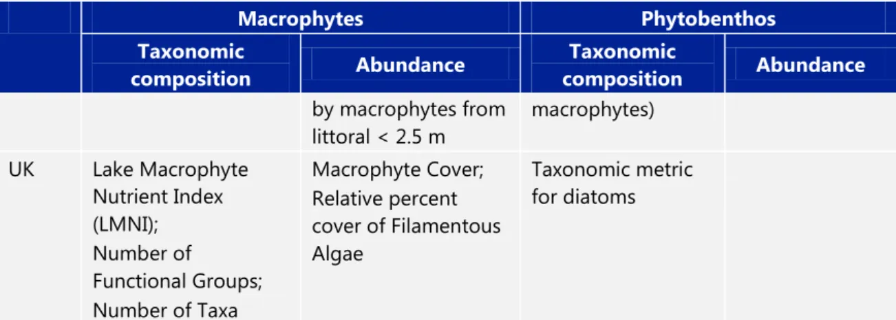
Table 2.2 Overview of the metrics included in the national macrophyte assessment methods. Macrophytes and phytobenthos intercalibrated separately

Macrophytes Phytobenthos

Taxonomic

composition Abundance

Taxonomic

composition Abundance BE_FL Type specificity score;

Disturbance score; Evaluation of number of present growth forms Submerged vegetation development (based on a four-class abundance scale) There is a separate diatom metric combined with the macrophyte metric (one out, all out).

Presence of cyanobacterial films and abundance of filamentous algae are accounted for in macrophyte metric calculations. DK Presence of indicator species; Depth limit of submerged plants in lakes with max depth >5 m. Total coverage (% of lake area) in lakes with max depth < 5 m

(7)

Macrophytes Phytobenthos Taxonomic composition Abundance Taxonomic composition Abundance EE Main hydrophyte groups in order of importance; Various indicators based on relative abundance of sensitive/tolerant taxa Depth limit of submerged plants (only LCB1) Abundance of large filamentous algae FR IBML : Indicator species (specific values + stenoecy coefficient) IBML : Relative abundance of hydrophyte, helophyte, macroalgae GE Reference Index; Total quantity of selected macrophyte taxa Total quantity of macrophytes Depth limit of macrophytes Trophic Index by Schönfelder Ratio of reference taxa Relative Abundance included in the trophic index LT Reference Index Depth limit (m) of

vegetation

(additional criteria)

- -

LV Presence of characteristic taxa and indicator species; Abundance of Charophyta, ceratophyllids and lemnids, Isoetids, Elodeids, floating-leaved plants, free-floating plants, helophytes, number of taxa

Colonisation depth, also see taxonomic composition Abundance of filamentous Chlorophyta NL Total score of characteristic species, depending on species indication value and species abundance.

Deviation of macrophytes cover from expected cover in suitable area under reference conditions (will probably be adjusted within intercalibration) No separate index; floating filamentous algae beds are incorporated into macrophytes growth forms PL Pielou index (eveness) Colonization index: relative proportion of total area occupied

Separate index for phytobenthos (not combined with

(8)

Macrophytes Phytobenthos Taxonomic composition Abundance Taxonomic composition Abundance by macrophytes from littoral < 2.5 m macrophytes) UK Lake Macrophyte Nutrient Index (LMNI); Number of Functional Groups; Number of Taxa Macrophyte Cover; Relative percent cover of Filamentous Algae Taxonomic metric for diatoms

MS use following combination rules:

 BE_FL - worst metric score; combination with phytobenthos score also as one out, all out;

 DK - sum of scores on indicator species and abundance metrics;

 EE - average of quality classes calculated for different indicators;

 FR - averaging of trophic score for littoral zone and perpendicular profiles. Weighted metric according the cover (%) of four predefined riparian types;

 GE - average metric scores (macrophytes and phytobenthos) per site. Averaging of sites for whole water body assessment;

 LT - average metric scores;

 LV - average of quality classes calculated for different indicators;

 NL - average of indicators for taxonomic composition and abundance;

 PL - in ESMI, the Pielou index and colonization index are combined into one formula, giving the results in a range from 0 (most disturbed) to 1

(reference, theoretical value);

 UK - weighted average of metrics for macrophytes, then take worst of macrophytes and diatom score.

For scientific literature and computation details see Annex F.1.

2.2. Sampling and data processing

Table 2.3 Overview of the sampling of the national macrophyte assessment methods MS Sampling device Surveyed _{compartment/habitat/ecotope} Abundance scale BE-FL A 50 cm broad

mesh-covered rake on a

telescopic handle (up to 4 m long)

A variable number of fixed transects, chosen to cover spatial variation as completely as possible, are sampled in deeper parts from a motor boat or by wading. Transect observations are

Species composition and abundance of individual macrophytes are estimated the scale from 1-5. Additionally,

(9)

MS Sampling device Surveyed _{compartment/habitat/ecotope} Abundance scale or a similar

double-sided rake fixed to a 20 m rope are used where necessary

supplemented by point observations to asses distribution patterns. If a boat is used in deep water, the double rake is thrown perpendicular to transect twice or three times on each side every 10 or 20 m; transect width is ca. 10 m.

the total abundance of submerged vegetation is estimated for each segment in 4 class scale, and the growth forms occurring in the water are listed.

DE SCUBA or by boat using a water viewer and a double rake with rope.

According to lake size and shape, usage of shore and catchment area 4 to 30 transects (=sites) are

investigated. Each transect covers a minimum of 20 m of homogeneous shoreline (=width), is divided into 0–1 m, 1–2 m, 2–4 m and >4 m depth classes and reaches from shore to vegetation limit (=variable length). If transects are investigated by a rake, at least five samples are taken in each depth class (20 samples per transect).

The species

composition uses a 5 classes of abundance, for each depth zone at each transect is recorded separately.

DK SCUBA diving or boat using a water viewer and a rake with a rope

Macrophyte data are obtained from transect investigations. Each lake is divided into a number of transects representing the whole lake area.

Macrophyte coverage at each observation point is estimated according to scale from 0 -6.

EE Plant hook (in very shallow water also rake),

observation tube Diving - rarely

Usually, small lakes are circled by boat, partly in deeper zone and along transects, partly in shallower zone near the water edge On the largest lakes of Peipsi (3555 km2_{) and Võrtsjärv (270} km2_{) monitoring is carried out on} transects.

Relative abundance are given according 5 abundance classes originally used by Braun-Blanquet, separately among three groups: helophytes, floating and floating-leaved plants, submerged plants FR a rake (with a

scaled handle) or a grapnel (with a scaled rope) are used according to the depth.

Bathyscope, Secchi disc and GPS device are also used

The macrophytes are sampled on observation units (1 section of shore and 3 perpendicular profiles). These observation units are located by applying the Jensen’s method (geometric positioning) and selected according the description of the shore such that the main types of riparian zone around the lake are represented.

Relative abundance in 5 class sale

(10)

MS Sampling device Surveyed _{compartment/habitat/ecotope} Abundance scale Aquascope perpendicular to shoreline transects

divided into 0–1 m, 1–2 m, 2–4 m and >4 m depth zones. At least three samples of macrophytes were taken from each depth zone (totally 3x4 per transect).

rare, 2 = rare, 3 = common, 4 = frequent and 5 = very frequent

LV The examination of the lake is

organized in transects. Passing the littoral of the whole lake by boat relative abundances of the macrophyte species of all belts and all taxonomical groups are estimated

Relative abundances of the macrophyte species in the 5 or 7 point scale

NL In most cases a double rake is used connected to a rope. In some cases snorkeling or estimation with the naked eye (clear and shallow water).

Each lake comprises 6 - 20 sampling points.

- In shallow, large lakes (> 500 ha) each sampling point has a size of 200x200m and is sampled at each corner 5 times with a rake.

- In smaller and medium lakes, as well as deeper lakes, 10 transects

perpendicular to the banks are sampled.

- Small lakes are sampled by random crossing the lake, aiming to record the complete species composition and estimate a total cover of growth forms.

Usually in a 9-classes cover scale for species and percentage for growth forms

PL In most cases a rake is used connected to a scaled rope

Number of transects depends on the area and the shape of the lake;

normally it makes one transect for app. 500m length of shoreline. The width of transect is about 20-30 m the length is from the shoreline to the max. depth of plant growth.

Share of each plant community in 7 point scale and % of total plant cover within a transect

UK 4 - 8 lake sectors should be surveyed depending on lake area . A sector should comprise a 100 metre length of shoreline. It should extend from the shore to the centre of the lake or to the maximum depth of colonisation of macrophytes. The sectors should be arranged to give an approximately equal spread around the perimeter of the lake.

Each indicator taxon present in the lake should be assigned a value (0 -100 %) which is an estimate of the percentage cover of the taxon in the area of the lake surveyed.

(11)

2.3. National reference conditions and class boundaries

Ecological status classifications of national methods were established individually by the Member States prior to the intercalibration process (see below).

Belgium:

 Contemporary references are absent for all types. The assessment is

therefore based on vegetation attributes estimated from the remaining sites presenting higher quality, historical records, and information on the

behaviour of species and the structural response of aquatic vegetations in relation to pressures, making as few assumptions as possible. This

information is integrated by expert judgement;

 Boundary values are set by expert judgement with the requirement that good status can only be attained if taxa which are not specific for the water type or show increased abundance with disturbance remain notably less abundant relative to type-specific and non-disturbance species.

Estonia:

 Reference lakes are not present in Estonia. Conception of high status is based on the data from the 1950s, or older data;

 H/G boundary is the state where the first signs of vegetation change appear;

 G/M boundary is the state where the representatives of H and G state are present, but not prevailing;

 The vegetation of the lakes on G/M boundary seems to be unstable.

Denmark:

 The method uses the total points score of two indicators, with a maximum of 4 points for indicator species and a maximum of 9 points for abundance (maximum colonized depth (LCB1) or total cover (LCB2)), resulting in a scale from 0-13 points;

 These have been assigned to ecological status classes, with 0-1 point = bad, 2-4 points = poor, 5-7 points = moderate, 8-10 points = good, and 11-13 points is high;

 The boundaries were set within the intercalibration process during the harmonization phase, by adjusting the score system for the two indicators. Germany:

 The reference is based on (few) existing reference sites;

 High Status: EQR values lie within the range of reference sites;

 Good Status: EQR values are slightly below high status and always positive (Taxa of species group A (sensitive taxa) have higher abundances than species group C (impact) taxa);

(12)

 Moderate: EQR values are around zero or negative (species group C taxa equal or slightly outweigh species group A taxa);

 Poor: EQR values are very low (species group A taxa are nearly replaced by species group C taxa);

 Bad: Very low macrophyte abundances without natural reasons. (Calculation of RI/EQR is often not possible).

Lithuania:

 For setting reference conditions, existing near-natural sites were chosen. These sites were selected according to expert knowledge, historical data and in which the least disturbed conditions are present. The criteria were: the absence or minimal human impact in the site or in all catchment area, the macrophyte community corresponds with description of reference

community description, diversity of macrophyte species corresponds with diversity of substrates, low quantity of nutrients, unaltered morphology and hydrology;

 In high alkalinity lakes cover of submerged vegetation with dominant Chara spp. is well developed. Sensitive submerged species are very abundant and dominant. Occurrence of tolerant and indifferent species is insignificant. The belt of helophytes and floating leaved plant not developed or very badly developed;

 Boundary setting: Preliminary ecological status boundaries estimated for German RI were used;

 In a "Good status" community the cover of Chara spp. in high alkalinity lakes is well developed and sensitive species have higher abundance than tolerant species, but are decreasing and replaced by tolerant and indifferent species. Netherlands:

 The number of reference sites is too low for setting reference values. Plant communities that are considered to be present in reference conditions are based on earlier work on target types in nature management (Bal et al.) and improved by expert judgement. The reference score for the sum of the scores of the species is derived from frequency data in this database;

 Class boundaries are expressed as percentage of the reference score -H/G 70%, G/M 40%, M/P 20%, P/B 10%;

 Final adjustment of the reference scores and class boundaries are based on intercalibration results.

Poland:

 Reference: median value of ESMI from real reference lakes identified according to the pressure criteria, for stratified and non-stratified lakes separately;

(13)

 H/G boundaries were determined as 75th percentile from the distribution of reference lakes;

 The whole range of ESMI from the H/G boundary to the minimum value was

divided in four classes in logarithmic scale;

 During the intercalibration process it became clear that boundary values for the G/M boundary were too relaxed in the case of both, stratified and non-stratified lakes. In a harmonization process it has been suggested to tighten the G/M and M/P boundaries by 20% and leave H/G boundary unchanged. UK:

Selection of reference sites:

 Putative reference sites were identified at a type-specific level initially from their biology, using individual species-pressure relationships indicated by empirical analysis, historical macrophyte records and expert opinion;

 Finally all reference sites were checked against available land cover, total P and chlorophyll data. Within-type regressions between pressures and biological metrics were used to identify sites where deviating biology was related to increased pressure. Any such outliers or sites with known hydromorphological modifications were then removed.

Individual metrics were modelled using environmental variables to determine their expected value at reference sites. These expected values are used to calculate an EQR for each metric. A multimetric EQR is then calculated based on the national combination rules.

National boundary setting:

 The H/G boundary corresponds to the lower 5th percentile of the multimetric EQR in reference sites and is interpreted as representing the lower limit of undisturbed status of the quality element;

 The GM boundary is based on the interval between the median EQR of the

national reference site dataset and the HG boundary and is approximately equivalent to the lower 1%tile of the reference site multimetric EQR. This point is interpreted to represent the limit of slight change in the quality element since there is some but minimal overlap with the natural variation in the population of reference sites;

 Below this the EQR range is divided equally to form the MP and PB boundaries.

Based on this information, the GIG considers that all methods are compliant with respect to macrophytes.

(14)

Table 2.4 Overview of the methodologies used to derive the reference conditions for the national macrophyte assessment methods

BE-FL Expert knowledge, historical data, least disturbed conditions DK Expert knowledge, historical data, least disturbed conditions

(no actual existing natural sites in lakes; spatial references from foreign countries) EE Existing near-natural reference sites, expert knowledge, historical data, least disturbed

conditions, modelling (extrapolating model results)

FR Existing least disturbed conditions sites following the criteria given in the National Circular DCE 2004/08.,

GE Existing near-natural reference sites, Expert knowledge, Historical data, Modelling (extrapolating model results), palaeo data (sediment-cores)

LT Existing near-natural reference sites, expert knowledge, historical data, least disturbed conditions

LV Existing near-natural reference sites, expert knowledge. NL Expert knowledge, historical data, least disturbed conditions

(no actual existing natural sites in lakes; spatial references from foreign countries) PL Existing near-natural reference sites, expert knowledge, least disturbed conditions UK Existing near-natural reference sites, Historical data, modelling (extrapolating model

results) Sites selected by iterative application of biological and physicochemical criteria, ca 600 surveys (mixture of historic and contemporary surveys)

Table 2.5 summarizes the methodology used to derive ecological class boundaries. Based on the information, the GIG considers that all methods are compliant with respect to macrophytes.

Table 2.5 Overview of the methodology used to derive ecological class boundaries BE-FL Equidistant division of the EQR gradient; reasoning behind it is not necessary a

linear scale for different metrics

DK DK use a point scale for different indicators; these are combined and translated to a EQR value, based on maximum colonization depth or cover, indicative species and total number of taxa

EE Using discontinuities in the relationship of anthropogenic pressure and the biological response and expert judgement. G/M boundary is the state where sensitive taxa are present, but not prevailing, other boundaries set proportional. FR H/G boundaries determined as 75th percentile from the distribution of reference

lakes divided over Alpine/LCB3 GIG. Equidistant division of continuum. GE The boundaries were set at the zones of distinct changes of the biocoenosis

(macrophytes and diatoms (eg Schaumburg et al 2004 etc)

LT Preliminary ecological status boundaries estimated for German RI were used LV Expert judgement based on ecological changes and normative definitions? NL Division of the EQR gradient as function of the total score for composition and the

abundance metric

(15)

lakes Division of the EQR gradient in original (not harmonised) method in logarithmic scale, differing between stratified and non-stratified lakes

UK Using paired metrics (sensitive and tolerant taxa) that respond in different ways to the influence of the pressure. EQR boundaries are subsequently adjusted to equidistant divisions.

3. Results of WFD compliance checking

The table below lists the criteria from the IC guidance and compliance checking conclusions.

Based on the information above, the GIG considers that all methods are compliant with respect to macrophytes. All methods show a significant correlation with eutrophication parameters.

Several countries (BE-FL, GE, UK, PL) have developed a separate metric for phytobenthos, others (NL, EE, LV) have included filamentous algae in their macrophyte metric, and argue that macrophytes taxonomic composition calculated this way and abundance are indicative for the quality element as a whole.

The GIG agrees in majority that macrophytes are indicative for the quality element as a whole for long-term changes and are responsive to the main anthropogenic pressures on lakes. It is acknowledged that phytobenthos can be used to detect short-term changes, but rapid year-to-year changes in maximum colonised depth for macrophytes as observed in many lakes also detect these short-term changes. Combination of these two would require intercalibrated separated metrics on the two before they can be combined.

Table 3.1 List of the WFD compliance criteria and the WFD compliance checking process and results

Compliance criteria Compliance checking conclusions 1. Ecological status is classified by

one of five classes (high, good, moderate, poor and bad).

Yes, fulfilled by all countries that have completed methods; except EE method does not distinct between Poor/Bad

2. High, good and moderate ecological status are set in line with the WFD’s normative definitions (Boundary setting procedure)

Yes, see table above

3. All relevant parameters

indicative of the biological quality element are covered (). A

combination rule to combine

para-meter assessment into BQE assessment has to be defined.

(16)

4. The water body is assessed against type-specific near-natural reference conditions?

Yes, see table above

5. Assessment results are expressed

as EQRs Yes, national EQR’s or classes can also be transformed to normalized (0-1) EQR’s. DK has discrete EQR values.

6. Sampling procedure allows for

representative information

about water body quality/ ecological status in space and time

In time: status is by all member states assessed per

sampled growing season (lake-years); For

macrophytes this is the appropriate time scale, with at least one sample during the peak of the growing season (June-Aug)

In space: yes, with use of transects and/or profiles or

mapping. Member states have rules for the % of shoreline or number of transects, often depending on size and heterogeneity of the lake.

7. All data relevant for assessing the biological parameters specified in the WFD’s normative

definitions are covered by the

sampling procedure

Parameters for abundance and species composition are covered, but are differing between countries.

8. Selected taxonomic level achieves adequate confidence and

precision in classification

All countries that have delivered data have determined at the desired species level, with few exceptions, such as charophytes in LV which are lumped. The adequate confidence and precision needs to be demonstrated during the phase where the assessments with the different national methods on the CBGIG database and/or with the common metrics are compared.

4. Results IC Feasibility checking

4.1. Typology

Intercalibration feasible in terms of typology - all assessment methods are appropriate for the common types LCB1 and LCB2 (see Table 4.1 and Table 4.2):

 All countries (except FR) share LCB1 and LCB2, therefore intercalibration is feasible for these two types;

 EE, DK, FR and LV have LCB3, and UK has lakes of similar type in the NGIG. However, this is insufficient for intercalibration within time frame due to large geographical differences and lack of data.

Only few countries have LCB3 lakes, but it was concluded within the GIG that even these few lakes were geographically too different to intercalibrate. Making

(17)

subcategories on LCB3 therefore is not possible due to the fact that this would give too small lake populations.

Table 4.1 Description of Lake Central/Baltic GIG common intercalibration types Common

IC type Type characteristics MS sharing IC common type LCB1 Shallow (3-15 m), alk > 1

meq/l

All countries except FR LCB2 Very shallow (<3 m), alk > 1

meq/l

All countries except FR LCB3 Shallow (3-15 m), alk < 1

meq/l

EE, LV & DK. UK has lakes of similar type in NGIG. FR has LCB3 lakes not comparable to the others due to geographic differences. IC for LCB3 not possible due to large geographical differences and lack of data.

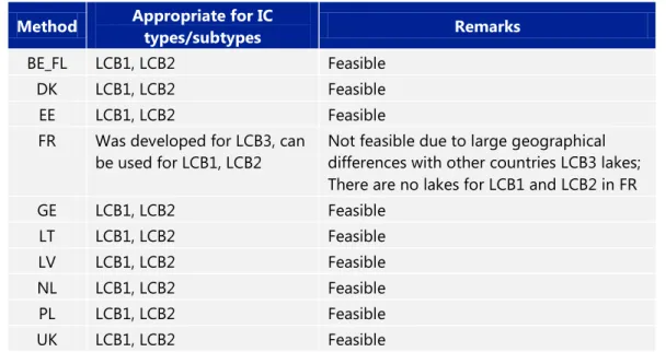
Table 4.2 Feasibility of IC of MS macrophyte assessment methods for IC common types Method Appropriate for IC _{types/subtypes} Remarks

BE_FL LCB1, LCB2 Feasible

DK LCB1, LCB2 Feasible

EE LCB1, LCB2 Feasible

FR Was developed for LCB3, can be used for LCB1, LCB2

Not feasible due to large geographical differences with other countries LCB3 lakes; There are no lakes for LCB1 and LCB2 in FR

GE LCB1, LCB2 Feasible LT LCB1, LCB2 Feasible LV LCB1, LCB2 Feasible NL LCB1, LCB2 Feasible PL LCB1, LCB2 Feasible UK LCB1, LCB2 Feasible

4.2. Pressures addressed

Lake macrophyte assessment methods addressed eutrophication + wide range of pressures :

 BE_FL method - eutrophication + wide range of pressures

(hydromorphology, habitat destruction, fish stocking, alien species);

 DK – eutrophication;

 EE - eutrophication + hydromorphological pressures;

 FR – eutrophication;

 GE - eutrophication + general degradation, habitat destruction;

(18)

 LV - eutrophication + wide range of pressures;

 NL - eutrophication + hydromorphological pressures;

 PL - eutrophication + also general degradation, organic pollution;

 UK – eutrophication.

Nevertheless, pressure-response relationships were developed only for eutrophication pressure. Hydromorphological pressures (water level fluctuations, residence time, lake shore morphology) are generally not well defined, both with respect to the pressure-response relationships and the monitoring of the pressures. This hampers the possibility to check pressure-response relationships

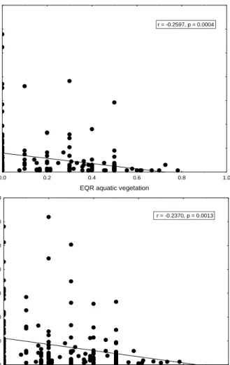
Intercalibration is feasible in terms of pressures addressed by the methods as all countries showed that their method responds significantly to eutrophication (TP, TN, Chlorophyll-a).

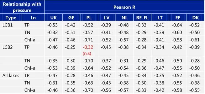
In the table below, the relationships of national methods with eutrophication variables TP, TN and chl-a are expressed as their Pearson R.

Table 4.3 Evaluation of IC feasibility regarding addressed pressures Relationship with pressure Pearson R Type Ln UK GE PL LV NL BE-FL LT EE DK LCB1 TP -0.53 -0.42 -0.52 -0.39 -0.48 -0.33 -0.41 -0.64 -0.52 TN -0.32 -0.51 -0.57 -0.41 -0.48 -0.29 -0.39 -0.60 -0.50 Chl-a -0.47 -0.46 -0.71 -0.52 -0.57 -0.28 -0.41 -0.58 -0.61 LCB2 TP -0.46 -0.25 -0.32 (n.s) -0.45 -0.38 -0.34 -0.34 -0.42 -0.39 TN -0.35 -0.30 -0.70 -0.37 -0.31 -0.29 -0.46 -0.50 -0.28 Chl-a -0.53 -0.39 -0.64 -0.52 -0.54 -0.36 -0.47 -0.55 -0.50 All lakes TP -0.47 -0.28 -0.46 -0.47 -0.45 -0.34 -0.35 -0.52 -0.46 TN -0.31 -0.35 -0.63 -0.43 -0.38 -0.30 -0.38 -0.55 -0.38 Chl-a -0.46 -0.36 -0.70 -0.56 -0.57 -0.33 -0.42 -0.58 -0.55 All relationships are significant at p<0.001, except PL for LCB2 with TP (R=-0.32, n=26, p=0.112)

4.3. Assessment concept

Intercalibration is feasible for assessment concept (see Table 4.4):

 However, not all indicators needed for all the national methods can be calculated for the common database. In those cases “compromised” versions of the national methods are used, and is it needed to demonstrate the

(19)

relationship between the “complete” and the “compromised” method as applied to the CBGIG database. If this relationship is insufficient, then preferably an option 2 comparison with common metrics can be used;

 Translation to national types based on the intercalibration database may be a source of uncertainty;

 Methods may be changed based on the intercalibration results; final methods and assessment concepts will be described as result of the intercalibration.

Table 4.4 Evaluation of IC feasibility regarding assessment concept of MS methods. Method Assessment concept

Method BE The method based on the following metrics:

 TS: type-specific species composition (relative abundance ratio) separately for riparian and aquatic vegetation;

 V: abundance of disturbance indicators (relative abundance ratio) separately for riparian and aquatic vegetation;

 GV: number of growth forms for aquatic vegetation only;

 VO: submerged vegetation development for aquatic vegetation only;

 riparian vegetation assessment considers all phreatophytes; aquatic vegetation assessment considers all hydrophytes and helophytes plus filamentous algae and cyanobacterial films up to a type-specific depth ( 2 m for LCB2;  4 m for LCB1)

Method DE The method based on the following metrics:

 Macrophytes reference index (RI): relative abundance of the

macrophyte species of three different type specific ecological species groups (reference indicators, indifferent taxa, degradation indicators; according to growth depth);

 limit of vegetation: used as an additional criteria;

 dominant stands: used as an additional criteria if a single species (e.g. Ceratophyllum demersum or Myriophyllum spicatum) reaches at least 80% of total plant quantity.

Method DK The method based on the following metrics:

 presence of indicator species

 Mean % cover submerged macrophytes (shallow lakes)

 Maximum growth depth (deep lakes) Method EE  Main hydrophyte taxa

 Relative abundance of Potamogeton perfoliatus or P. lucens among submergents

 Relative abundance of charophytes or bryophytes among submergents

 Relative abundance of Ceratophyllum among submergents or of lemnids among nymphaeids& lemnids

(20)

Method Assessment concept

 Maximum colonization depth (LCB1 only)

 Maximum depth of mosses (only LCB3 with depth>3 m)

Method FR IBML method : Relative abundance of indicator taxa (specific value + stenoecy coefficient) including hydrophytes, helophytes and macroalgae (riparian + water) Method LT Reference Index calculated according to Lithuanian list of indicatory species (A –

sensitive, C–insensitive and B – indifferent taxa) and named L-RI. Depth limit (m) of vegetation (additional criteria)

Index is calculated fore each transect and calculation is based on list of taxa and its abundance, estimated at different depth zones.

Adapted from German method using modified specific list of LT species; uses occurrence of species in different depth zones

Method LV The method based on the following metrics: characteristics species, indicator species, macrpjhyte species number, abundance of charophytes, isoetids, elodeids, freely floating species, nympheids, green algae, colonisation depth

Method PL The method based on the following metrics:

 Pielou index of evenness of species distribution

 area covered relative to area with depth < 2.5 m

 Phytobenthos index is a separate assessment not part of macrophyte based assessment. No integration rules at the moment

Method NL The method based on the following metrics:

 total sum of abundance related scores of all species encountered

 covered area compared to potential area (area with depth <2.7 m in LCB2; area with depth < 4.5 m in LCB1)

 covered area of helophytes relative to potential area Method UK The method based on the following metrics:

 Lake Macrophyte Nutrient Index (LMNI);

 Number of functional groups of macrophyte taxa (NFG).

 Number of macrophyte taxa (NTAXA);

 Mean percent cover of hydrophytes (COV);

(21)

5. IC dataset collected

Huge dataset was collected within the CB macrophyte GIG, including 254 lake years from LCB1 (8 MS) and 274 lake years from LCB2 (9 MS), see tables below.

Table 5.1 Description of data collection within the GIG per MS

Member State Macrophyte data Chlorophyll TotalP TotalN

LCB1 lake type BE 5 4 5 5 DK 25 19 21 21 EE 13 8 12 12 GE 32 32 32 0 UK 21 20 14 18 LV 67 67 66 55 NL 14 14 14 7 PL 77 71 77 77 LCB2 lake type BE 14 4 6 6 DK 62 55 56 56 EE 13 9 10 12 GE 18 16 18 0 UK 39 38 31 32 LT 21 21 21 21 LV 45 45 45 39 NL 36 36 36 19 PL 26 26 26 26

Table 5.2 Distribution of CB lakes in the CB Macrophyte GIG database across quality classess LCB1 LCB2 LCB3 total High 16 7 3 26 Good 61 43 5 109 Moder 28 45 5 78 Poor 5 17 0 22 Bad 7 23 3 33 Unknown 101 112 46 259 total 218 247 62 527 U=Unknown

(22)

Table 5.3 List of the data acceptance criteria used for the data quality control and the data acceptance checking

Data acceptance criteria

Data acceptance checking Data requirements

(obligatory and optional)

Abundances are determined at the species level; genus level may be acceptable if this does not hamper assessment by other methods (this is the case with charophytes in Latvian lakes); supporting physico-chemical data and lake characteristics should be provided. The GIG used a template in the date request that was filled by all member states providing data.

The sampling and analytical

methodology

Member states use different scales for abundance of macrophytes species. UK and PL use a continuous scale, the other member states use point scales with a variable number of classes. DK use

presence/absence data for species composition. Conversion from one scale to another was done by a conversion table based on the

description of the various abundance scales as provided by the member states, and agreed within the group.

Level of taxonomic precision required and taxalists with codes

An extended taxon list (compared to that of the 1st round) was used, containing 173 species. Countries provided data on missing species that are used in their national methods

The minimum number of sites/samples per intercalibration type

For LCB1 and LCB2 there are sufficient sites in the database. For LCB3 this is not the case, and it is intended to combine LCB3 with similar types from the NGIG.

France has 3 sites in CBGIG (only LCB3). Sufficient covering of

all relevant quality classes per type

Preliminary status assessment of national methods on their own lakes shows that for LCB1 a large fraction of lakes is assessed high or good. For LCB2 the majority is assessed as good or moderate, with few lakes assessed s high status. Many lakes (from countries with no method and from LV) were not assessed. Especially LV may have more LCB2 lakes in high status.

6. Common benchmarking

The intercalibration dataset does contain reference sites as assigned by the member states. However, their number is considered to be insufficient, and also the TP and chlorophyll-a range of the assigned reference sites is considered quite broad (see Figure 6.1). Therefore other approaches as alternative benchmarks or continuous benchmarking were considered.

Graph below shows that the assigned reference sites have a relatively broad spread of TP and chl-a values, but that there are many more sites with comparable TP and chl-a values.

(23)

Also alternative benchmarking was not possible because of limited number of sites within a narrow range of pressure. Therefore continuous benchmarking was used:

 The list of sites with a range of TP (0–0.2 mg P/l) were included for the continuous benchmarking;

 These lakes provide a sufficient number of benchmarking sites and sufficient geographical distribution within the CBGIG (together 426 lakes - 222 LCB1 and 204 LCB2 lakes);

 There is sufficient spread of sites over eastern and western part of GIG;

 For each combination of the application of method from MS A to the lakes of MS B a benchmark correction factor to the standardised EQR was calculated (see table below).

Figure 6.1 Range of TP and chl-a values of Central/Baltic GIG reference sites. Table 6.1 Benchmark standardization correction factors

MS assesment method Lakes UK DE PL LV NL BE LT EE DK UK -0.03 -0.03 -0.05 -0.01 -0.09 -0.02 0.03 -0.01 DE -0.05 0.05 0.05 0.03 0.05 0.05 PL -0.01 -0.03 0.00 -0.01 -0.03 0.15 -0.04 -0.03 -0.03 LV 0.07 0.09 -0.01 0.01 -0.01 0.10 0.07 0.09 NL -0.09 -0.01 0.01 -0.01 -0.09 0.04 -0.09 -0.05 BE -0.05 -0.03 0.01 0.05 0.15 -0.18 0.05 0.01 LT 0.07 0.01 -0.17 -0.07 0.06 -0.05 EE 0.09 -0.03 0.03 0.09 0.05 -0.04 -0.01 0.09 DK -0.03 -0.05 0.05 -0.01 -0.15 -0.10 -0.05 0 20 40 60 80 0.00 0.02 0.04 0.06 0.08 0.10 chl -a (u g /l) TP (mg/l)

all lakes ref sites LCB1 ref sites LCB2 ref sites LCB3

(24)

Explanations:

 Empty fields imply that a method was not applied to the lakes of the corresponding country;

 The benchmark factor for application of the BE_FL method to the BE-FL lakes was corrected to 0.0 based on the estimated systematic bias between full BE-FL method applied to Belgian lakes and the compromised BE-FL method applied to all other lakes;

 The PL method was only applied to PL lakes. Intercalibration of the PL method was possible nonetheless, because large number of PL lakes in CB-GIG database (n=99).

7. Comparison of methods and boundaries

IC Option and Common Metrics

Intercalibration “Option 3” was used - direct comparison of assessment methods using a common dataset via application of all assessment methods to all data available. However, not all indicators needed for all the national methods can be calculated for the common database. In those cases “compromised” versions of the national methods are used, and is it needed to demonstrate the relationship between the “complete” and the “compromised” method as applied to the CBGIG database.

If insufficient agreement was reached between the full MS method and the “compromised” method that can be applied to the CBGIG database, then a method was only applied to the member state’s own lakes. This is the case for PL (the missing information on helophytes and depth distribution compromised the PL method too much, so the full PL method was applied only to PL lakes). In case of BE-FL (unable to calculate 1 out of 4 metrics: the abundance metric), a correction factor was applied. For comparison of the MS assessments, a pseudo-common metric based on the average of the benchmark corrected standardised EQR’s of all other member states. Methods harmonization process

Some methods initially had a low correlation (UK, DE, BE-FL) but during the harmonization process these were improved. Before final calculation a number of steps have been performed:

 Because the Polish method had to be compromised too much it was

decided that PL could use their full method applied only to the PL lakes. This was possible because of a sufficiently large number of PL lakes in CBGIG database (n=99);

 The Latvian assessments were slightly changed by calculation of index for characteristic taxa;

(25)

 UK method was applied to German lakes based on estimates of alkalinity from total hardness  for UK overall correlation decreased from R=0.5 to R=0.4;

 Adaptation of NL method to include abundance metric  NL metric became less precautionary;

 French method was not taken into account due to lack of lakes and data in the LCB1 and LCB2 type  this lowered correlation for UK, but improve it for EE, also PL method became relatively too loose (boundary bias increased to +0.38);

 Germany have adapted their method to meet with criteria for correlation with the pseudo common metric;

 NL have adjusted scoring system for individual metrics within their method;

 DK have adjusted their method (no longer use metric on total number of taxa, have adjusted class boundaries for abundance and indicator species;

 UK has provided new method, to comply with criteria for correlation with pseudo common metric and pressure.

Furthermore, additional changes were performed:

 DK method was further adjusted with respect to class boundaries for individual indicators,

 Class EQR boundaries were adjusted where needed (PL, EE, GE) to make

countries comply with comparability criteria for HG and GM boundary bias.

 BE-FL have further adjusted their results by screening the assignment of lakes from the CBGIG database to the national BE-FL types. This resulted in a change of national type for 4 PL lakes, which improved the correlation with the PCM brought the HG boundary bias for LCB2 within the accepted range, and that for LCB1 very close to the lower limit for acceptance, at -0.27;

 UK have adjusted their G/M boundary from 0.67 to 0.66 for both LCB1 and

LCB2. This made the UK method less precautionary for LCB1, although still more precautionary than needed, while for LCB2 and LCB1&LCB2 combined all boundary biases remain within the accepted range. As the UK method does not distinguish between LCB1 and LCB2, the combined LCB1&LCB2 results should be used. This adjustment also moves the LCB1 H/G boundary bias for BE-FL further up from -0.27 to -0.25, bringing it just within the accepted range.

Results of the regression comparison (National EQRs vs. common metrics)

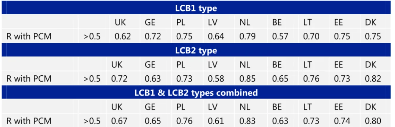
After several adjustments (UK, BE-FL, DE methods) for all Member States (and for LCB1, LCB2 as well as LCB1 and LCB2 types combined) correlation between national methods and pseudo-common metrics is significant at least at p<0.001 (and usually much smaller p-value).

(26)

Table 7.1 Correlation coefficients (R) for the relationship of each method with the pseudo-common metric (PCM). LCB1 type UK GE PL LV NL BE LT EE DK R with PCM >0.5 0.62 0.72 0.75 0.64 0.79 0.57 0.70 0.75 0.75 LCB2 type UK GE PL LV NL BE LT EE DK R with PCM >0.5 0.72 0.63 0.73 0.58 0.85 0.65 0.76 0.73 0.82 LCB1 & LCB2 types combined

UK GE PL LV NL BE LT EE DK

R with PCM >0.5 0.67 0.65 0.76 0.61 0.83 0.63 0.73 0.74 0.80 The pseudo-common metric is also significantly correlated (all p<<0.001) with TP for all countries. Note: these differ only slightly between countries, as they are the average of the assessments by all methods minus one

Table 7.2 Correlation coefficients (Pearson R) for the relationship of the pseudo-common metric (PCM) with total phosphorus (TP).

MS UK GE PL LV NL BE LT EE DK

Pearson R -0.53 -0.55 -0.56 -0.52 -0.56 -0.56 -0.56 -0.53 -0.55

n 423 481 481 423 481 434 480 471 481

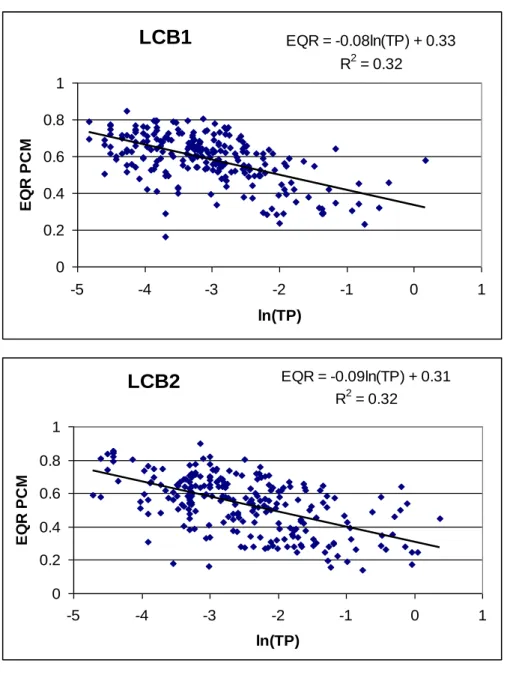
The overall PCM (avg of EQRs of all intercalibrated methods) is also significantly correlated to TP for both LCB1 and LCB2 (Figure 7.1).

(27)

Figure 7.1 Relationships between TP and the overall PCM (avg of EQRs of all intercalibrated methods) for common lake types LCB1 and LCB2.

7.1. Evaluation of comparability criteria

Finally a class comparison was made by comparing the classifications when each method was applied to as many countries as possible (Option 3a).

The absolute class difference was calculated. In all cases the methods achieved the comparability criteria of <1.0 absolute class difference, ranging from 0.6 to 0.8, average 0.69 (see Table 7.3)

LCB1

EQR = -0.08ln(TP) + 0.33 R2 = 0.32 0 0.2 0.4 0.6 0.8 1 -5 -4 -3 -2 -1 0 1 ln(TP) E Q R P C M

LCB2

EQR = -0.09ln(TP) + 0.31 R2 = 0.32 0 0.2 0.4 0.6 0.8 1 -5 -4 -3 -2 -1 0 1 ln(TP) E Q R P C M

(28)

Boundary bias was calculated (see

Table 7.3):

 LT, LV and UK have a positive boundary bias exceeding 0.25 class limit - means that these methods are precautionary with respect to the average boundary of all MS

 UK complies based on combined LCB1 and LCB2 results (as UK boundaries

are too precautionary only for LCB1 lakes;

 LV and LT have agreed to keep their relatively strict class boundaries.

Table 7.3 Overview of the IC comparability criteria Compliance criteria Limit Type LCB1 UK GE PL LV NL BE-FL LT EE DK Class agreement <1.0 0.69 0.68 0.63 0.72 0.60 0.74 0.66 0.63 0.64 HG Bias -0.25 +0.25 0.36 0.20 -0.09 -0.22 0.07 -0.25 0.69 -0.21 0.20 GM Bias -0.25 +0.25 0.27 0.03 -0.13 -0.23 -0.03 -0.02 0.42 -0.10 0.15 Compliance criteria Limit Type LCB2 UK GE PL LV NL BE-FL LT EE DK Class agreement <1.0 0.73 0.65 0.70 0.77 0.67 0.78 0.80 0.68 0.70 HG Bias -0.25 +0.25 -0.12 -0.12 0.04 0.27 0.08 -0.18 0.47 0.05 0.22 GM Bias -0.25 +0.25 -0.12 -0.24 -0.08 0.18 0.09 -0.01 0.56 0.21 0.17 Compliance criteria Limit

Types LCB1 & LCB2 combined

UK GE PL LV NL BE-FL LT EE DK Class

agreement <1.0 0.71 0.66 0.65 0.75 0.63 0.76 0.73 0.66 0.67 HG Bias -0.25 +0.25 0.08 -0.05 0.02 0.01 0.10 -0.17 0.55 -0.06 0.25 GM Bias -0.25 +0.25 0.05 -0.18 -0.07 -0.02 0.05 -0.02 0.52 0.08 0.18 Class boundaries to be included in the IC Decision

Table 7.4 Ecological quality ratios of national classification systems intercalibrated Member

State

National classification systems intercalibrated

IC type

Ecological Quality Ratios High-good boundary Good-moderate boundary Belgium (Flanders)

Flemish macrophyte assessment

system All types 0.80 0.60

Denmark Danish Lake Macrophytes Index All types 0.80 0.60 Estonia Estonian surface water ecological LCB1 0.78 0.52

(29)

Member State

National classification systems intercalibrated

IC type

Ecological Quality Ratios High-good boundary Good-moderate boundary quality assessment – lake

macrophytes LCB2 0.76 0.50

Germany Verfahrensanleitung für die

ökologische Bewertung von Seen zur Umsetzung der

EG-Wasserrahmenrichtlinie:

Makrophyten und Phytobenthos (Phylib), Modul Makrophyten

All types 0.80 0.60

Lithuania Lithuanian macrophyte assessment

method All types 0.75 0.50

Latvia Latvian macrophyte assessment

method All types 0.80 0.60

Netherlands WFD-metrics for natural water types All types 0.80 0.60 Poland Macrophyte based indication method

for lakes - Ecological Status

Macrophyte Index ESMI (multimetric)

All types 0.68 0.41 United

Kingdom

LEAFPACS lake macrophyte

classification tool* All types 0.80 0.66

*Will be used in England, Wales and Scotland

Table 7.5 Correspondence between common intercalibration types and common boundaries to the national typologies/assessment systems

LCB1 LCB2

BE-FL Type AW-e, AW-om Type Ai

Types AMI-e, AMI-om DE Type TKg 13

Type TKg 10

Type TKp

DK Type 10 Type9

EE Type III Type II

LT Type II Type III Type I LV Type 5 Type 6 Type 9 Type 1 Type 2 NL M20 M21 M14 M27 PL Part of 2a, 3a, 5a, 7a (only stratified with

mean depth >3)

Part of 2b, 3b, 4, 5b, 6b, 7b (only non-stratified with mean depth <3) UK HAS (alk > 0.1mEq/l, depth 3-15 m) HAVS (alk >0.1mEq/l, depth < 3m)

(30)

The harmonisation process to meet the comparability criteria for the different MS methods has been completed

8. Description of IC type-specific biological communities

The GIG has described taxa descriptive for high and good status on one hand, and taxa descriptive for less than good status (moderate, poor, bad). In summary:

 This has resulted in a list of taxa that occur for more than 2/3 in lakes with EQR of the PCM >0.6. This list contains many charophyte taxa and a number of Potamogeton species, as well as several others. These are the taxa that are according to the common view of the member states, considered as descriptive for good and high status, and are included in the indicators for good ecological status used by the national methods, and that disappear with decreasing PCM.

 On the other hand there is a large number of taxa that occur both at PCM>0.6 and PCM<0.6. These are considered the tolerant taxa. There are very few taxa that mainly (>2/3) occur at PCM<0.6.

 To describe borderline communities is considered an inherent impossibility, as at these borderlines the changes occur, and there is usually a mixture of species indicative for good and moderate status.

Background

As part of the 2nd_{phase of intercalibration, the GIGs are required to provide a narrative}

description of communities at borderline conditions between Good and Moderate status. However, since borderline conditions reflect a transition between good and moderate conditions and therefore reflect the position along the gradient where large changes in the presence of taxa occur, a description of borderline communities themselves seems an inherent impossibility. Therefore it was agreed (Ecostat, October 2011) that GIGs can instead provide a narrative description of communities at high, good and less than good status, with a list of taxa that show preference for these conditions. Then the emphasis can be put on the differences between taxa occurring at high, good and less than good status. This then reflects the (dis)appearance and of taxa along the EQR gradient and the pressures that the EQR is responsive to.

This section provides the analysis to come to a more narrative description of the common view of the member states participating in the Central-Baltic GIG lake macrophytes group of what macrophyte communities look like under good and moderate status

Selection of taxa to describe high, good and moderate conditions

We analysed the frequency distribution of taxa over the gradient of the PCM (= pseudo common metric, which is the average standardised EQR of all available assessments by

(31)

all intercalibrated member state methods after benchmark standardisation). This frequency distribution was calculated from the lake(year)s in which the taxa were found, Taxa occurring mainly at PCM>0.8 are considered indicative for high status, taxa occurring mainly at a PCM 0.6 - 0.8 to be descriptive for Good status, and taxa occurring mainly at PCM<0.6 Taxa occurring over the whole PCM gradient are considered to be insensitive.

Method

The CBGIG Macrophytes common database was used for this analysis. Assessments of lakes by all intercalibrated member states methods (BE-FL, UK, NL, DK, GE, PL, LT, LV, EE) were transformed to standardised EQR values and corrected for country effects by continuous benchmark standardisation. The average EQR of all assessments is referred to as the PCM (scale 0-1, with H/G boundary at EQR=0.8; G/M boundary at EQR=0.6). The gradient along this PCM is used for further analysis of the occurrence and disappearance of taxa.

For all taxa the lowest, 25-percentile, median(=50%-percentile), 75-percentile, and highest PCM value of the lake years in which a taxa occurred were calculated. Only taxa that occurred in at least 7 lake(year)s for either LCB1 and LCB2 from the CBGIG common database were selected.

Frequency distributions of taxa on the PCM scale were calculated from the number of lake(year)s with PCM>0.6 (good and high status) and PCM<0.6 (moderate, poor and bad status).

Results and discussion

The lowest, 25-percentile, median(=50%-percentile), 75-percentile, and highest PCM value of individual taxa are listed in Table 8.1 (LCB1) and (LCB2), where taxa are sorted after their median values. Taxa in the upper parts of Table 8.1 and have the highest frequency of occurrence at less than good status (median value <0.6). However, most taxa even in the upper part of the Table 8.1 and Table 8.2 also occur for a considerable fraction at PCM >0.6, and none of them have a median below 0.5. They therefore cannot be considered as descriptive for less than good status, but rather as taxa indifferent to the PCM value and hence for the pressures to which the PCM is responsive.

On the other hand there is a considerable number of taxa in the lower parts of the tables, with high median PCM that can be considered as descriptive for Good status. They occur only for a small part at PCM’s < 0.6. These reflect the taxa that disappear from the communities going down the PCM gradient. There are no taxa found to be exclusively descriptive for High status. This may be due to the relatively small number of lake years in the CBGIG database with PCM>0.8.

Many taxa however show a wide distribution over the PCM gradient.

The selection of descriptive taxa is based on frequency of occurrence at either PCM>0.6 and PCM<0.6, Taxa are considered descriptive for less than good status if more than

(32)

2/3 of the lake-years in which they occur have a PCM < 0.6. Taxa that are considered descriptive for good status are selected if more than 2/3 of the lake-years in which they occur have a PCM>0.6.

With these criteria, 39% and 32% of the taxa in Table 8.1 and Tbel 8.2. are considered descriptive for good and high status in LCB1 and LCB2 respectively. On the other hand only one out of 61 taxa is descriptive for less than good status in LCB1, and only 6 out of 58 for LCB2, including filamentous algae (Table 8.4).

The number of sites where the pseudo common metric was >0.8 is quite small to do a similar analysis for high status. Also, the taxa that are descriptive for good status tend to occur at the PCM range from 0.6 up to the maximum. Taxa that are indicative solely for high status can therefore not be assigned, but would be a subset of the list in Table 8.3, where taxa closest to the bottom in Table 8.1 and Table 8.2. are the most indicative for high status.

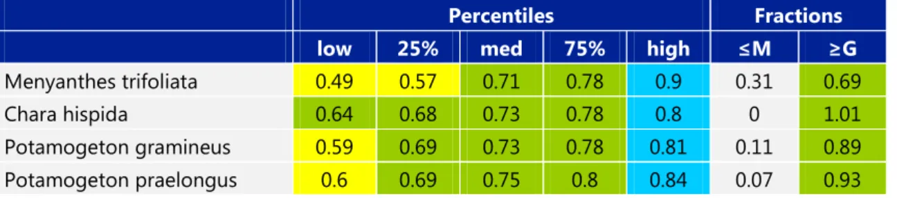
The majority of the taxa descriptive for good status are the same for LCB1 and LCB2 (Table8.3). Some taxa were found to be descriptive for only one lake type.

Most of the taxa selected as descriptive for good status could be expected into this selection because they are generally incorporated in national metrics as indicators for good ecological status (mainly charophytes and several Potamogeton species), and therefore reflect the common view of the member states on what macrophyte communities in lakes should look like. The national assessment methods only use to a lesser extent taxonomic indicators for moderate, poor or bad status (these states are mainly associated with a reduction of macrophyte abundance). This is reflected in the small number of taxa that were selected as descriptive for less than good status..

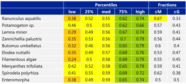
Table 8.1 Percentiles of taxa along the PCM gradient for LCB1. Taxa are sorted to increasing median value. Cells in columns with percentiles are coloured according to their quality classes (red = bad, orange = poor, yellow = moderate, green = good, blue =high). Cells in columns with fractions for status ≤M and ≥G are coloured yellow and green respectively when they are > 0.66.

Percentiles Fractions

low 25% med 75% high ≤M ≥G

Ranunculus aquatilis 0.38 0.52 0.55 0.62 0.74 0.67 0.33 Potamogeton sp. 0.46 0.5 0.55 0.62 0.66 0.57 0.43 Lemna minor 0.29 0.49 0.56 0.67 0.74 0.59 0.41 Zannichellia palustris 0.35 0.53 0.56 0.7 0.79 0.56 0.44 Butomusumbellatus 0.32 0.46 0.56 0.65 0.79 0.6 0.4 Elodea nuttallii 0.35 0.49 0.57 0.69 0.76 0.53 0.47 Filamentous algae 0.24 0.5 0.58 0.69 0.79 0.55 0.45 Menyanthestrifoliata 0.42 0.52 0.58 0.65 0.79 0.59 0.41 Spirodela polyrhiza 0.41 0.55 0.59 0.69 0.72 0.62 0.38 Enteromorpha 0.38 0.49 0.59 0.65 0.74 0.5 0.5

(33)

low 25% med 75% high ≤M ≥G

Persicaria amphibia 0.29 0.51 0.59 0.67 0.79 0.52 0.48 Sparganium erectum 0.28 0.5 0.6 0.65 0.79 0.53 0.47 Nuphar lutea 0.28 0.52 0.6 0.67 0.8 0.53 0.47 Nymphaea alba 0.32 0.52 0.6 0.67 0.79 0.51 0.49 Ceratophyllum demersum 0.17 0.55 0.62 0.68 0.85 0.46 0.54 Nymphaea candida 0.51 0.57 0.62 0.69 0.8 0.46 0.54 Hydrocharis morsus-ranae 0.17 0.55 0.62 0.66 0.77 0.48 0.53 Sparganiumemersum 0.35 0.57 0.62 0.68 0.74 0.47 0.53 Nuphar pumila 0.41 0.55 0.62 0.68 0.79 0.47 0.53 Schoenoplectuslacustris 0.29 0.55 0.62 0.68 0.8 0.45 0.55 Potamogeton crispus 0.46 0.53 0.62 0.68 0.79 0.47 0.53 Potamogeton perfoliatus 0.35 0.55 0.63 0.7 0.85 0.42 0.58 Potamogeton obtusifolius 0.53 0.56 0.63 0.7 0.75 0.38 0.63 Ceratophyllum submersum 0.17 0.57 0.63 0.69 0.77 0.36 0.64 Lemna trisulca 0.46 0.59 0.63 0.69 0.79 0.33 0.67 Myriophyllum spicatum 0.32 0.56 0.64 0.7 0.8 0.38 0.62 Potamogeton natans 0.41 0.57 0.64 0.7 0.8 0.38 0.62 Ranunculuslingua 0.52 0.59 0.64 0.66 0.68 0.38 0.63 Elodea canadensis 0.24 0.54 0.64 0.69 0.79 0.38 0.62 Ranunculus circinatus 0.42 0.56 0.64 0.7 0.8 0.35 0.65 Chara sp. 0.39 0.59 0.64 0.68 0.79 0.29 0.71 Potamogeton berchtoldii 0.53 0.58 0.64 0.68 0.79 0.4 0.6 Myriophyllum verticillatum 0.5 0.6 0.64 0.72 0.85 0.32 0.68 Sagittariasagittifolia 0.35 0.58 0.64 0.7 0.79 0.36 0.64 Potamogeton pusillus 0.39 0.54 0.64 0.73 0.79 0.43 0.57 Potamogeton pectinatus 0.29 0.56 0.64 0.7 0.85 0.35 0.65 Potamogeton trichoides 0.49 0.6 0.65 0.74 0.79 0.31 0.69 Potamogeton lucens 0.45 0.58 0.65 0.71 0.8 0.34 0.66 Potamogeton compressus 0.52 0.58 0.65 0.69 0.79 0.4 0.6 Fontinalisantipyretica 0.44 0.6 0.65 0.7 0.8 0.26 0.74 Najas marina 0.42 0.61 0.65 0.73 0.85 0.24 0.76 Charavirgata 0.46 0.59 0.66 0.71 0.85 0.3 0.7 Myriophyllum alterniflorum 0.42 0.57 0.66 0.74 0.76 0.36 0.64 Stratiotes aloides 0.41 0.61 0.66 0.71 0.85 0.25 0.75 Chara vulgaris 0.54 0.64 0.66 0.73 0.79 0.09 0.91 Chara globularis 0.48 0.63 0.66 0.73 0.79 0.22 0.78 Utricularia 0.48 0.59 0.67 0.71 0.8 0.29 0.71 Chara fragilis 0.53 0.63 0.67 0.73 0.79 0.12 0.88

(34)

low 25% med 75% high ≤M ≥G

Utricularia vulgaris 0.49 0.63 0.68 0.71 0.79 0.24 0.76 Potamogeton friesii 0.59 0.64 0.68 0.72 0.79 0.06 0.94 Potamogeton praelongus 0.51 0.62 0.68 0.71 0.79 0.18 0.82 Charophyta 0.39 0.63 0.69 0.73 0.85 0.16 0.84 Eleocharis acicularis 0.46 0.51 0.69 0.7 0.74 0.43 0.57 Nitellopsis obtusa 0.55 0.64 0.7 0.75 0.85 0.11 0.89 Chara aspera 0.59 0.63 0.71 0.75 0.79 0.2 0.8 Chara contraria 0.54 0.66 0.71 0.75 0.85 0.1 0.9 Chara tomentosa 0.57 0.68 0.73 0.76 0.79 0.13 0.88 Potamogeton filiformis 0.61 0.66 0.73 0.78 0.85 0 1 Chara rudis 0.59 0.64 0.73 0.77 0.85 0.08 0.93 Nitella flexilis 0.61 0.69 0.73 0.76 0.79 0 1 Chara hispida 0.6 0.72 0.76 0.77 0.79 0.11 0.89

Table 8.2 Percentiles of taxa along the PCM gradient for LCB2. Taxa are sorted to increasing median value. Cells in columns with percentiles are coloured according to their quality classes (red = bad, orange = poor, yellow = moderate, green = good, blue =high). Cells in columns with fractions for classes ≤M and ≥G are coloured yellow and green respectively when they are >0.66.

low 25% med 75% high ≤M ≥G

Lemnaminuta 0.3 0.34 0.51 0.62 0.82 0.7 0.3 Persicaria amphibia 0.28 0.44 0.53 0.61 0.74 0.73 0.27 Sparganium erectum 0.17 0.38 0.54 0.65 0.9 0.64 0.36 Nymphoides peltata 0.42 0.52 0.54 0.62 0.73 0.67 0.33 Lemna minor 0.27 0.42 0.54 0.64 0.84 0.66 0.35 Filamentous algae 0.22 0.48 0.56 0.64 0.78 0.69 0.31 Nymphaea alba 0.31 0.49 0.56 0.67 0.9 0.61 0.38 Zannichellia palustris 0.28 0.48 0.56 0.64 0.8 0.68 0.32 Elodea nuttallii 0.32 0.51 0.57 0.63 0.82 0.65 0.35 Enteromorpha 0.19 0.49 0.57 0.66 0.71 0.64 0.36 Nuphar pumila 0.38 0.52 0.57 0.69 0.76 0.6 0.4 Callitriche agg. 0.29 0.5 0.58 0.66 0.77 0.63 0.38 Potamogeton pusillus 0.39 0.52 0.58 0.65 0.8 0.56 0.44 Potamogeton crispus 0.27 0.5 0.58 0.66 0.8 0.54 0.46 Nuphar lutea 0.17 0.49 0.58 0.66 0.9 0.58 0.42 Sagittariasagittifolia 0.31 0.52 0.58 0.64 0.77 0.68 0.32