Publication date 2018
Original citation Griffith, J. 2018. An analysis of collaborative filtering datasets. PhD Thesis, University College Cork.
Type of publication Doctoral thesis
Rights © 2018, Josephine Griffith.
http://creativecommons.org/licenses/by-nc-nd/3.0/
Embargo information No embargo required Item downloaded
from http://hdl.handle.net/10468/5532
Filtering Datasets
Josephine Griffith
B.Sc., National University of Ireland, Galway 1994
M.Sc., National University of Ireland, Galway, 1997
NATIONAL UNIVERSITY OF IRELAND, CORK
Faculty of Science
Department of Computer Science
Thesis submitted for the degree of
Doctor of Philosophy
January 2018
Head of Department: Prof. Cormac J. Sreenan Supervisor: Humphrey Sorensen
Contents
List of Figures . . . v
List of Tables . . . vii
Abstract . . . xiii
Acknowledgements . . . xv
1 Introduction and Overview 1 1.1 Motivations . . . 1
1.2 Open Research Problems . . . 2
1.3 Aims . . . 3
1.4 Research Challenges . . . 3
1.5 Methodology . . . 4
1.6 Contributions . . . 4
1.7 Thesis Overview . . . 5
2 The Case for Collaborative Filtering 7 2.1 Introduction . . . 7
2.2 Motivations of Collaborative Filtering Research . . . 8
2.3 Collaborative Filtering: An Overview . . . 9
2.4 U: The Users; I: The Items and P: The Dataset . . . 10
2.5 M: The Collaborative Filtering Models . . . 12
2.5.1 Memory-based Models . . . 12 2.5.2 Graph Models . . . 14 2.5.3 Probabilistic Models . . . 14 2.5.4 Combination . . . 16 2.5.5 Weighting Schemes . . . 17 2.5.6 Learning . . . 18 2.6 R(I, u): Recommended Items . . . 18
2.6.1 Predictive Accuracy Focus . . . 19
2.6.1.1 Error-based Approaches . . . 19 2.6.1.2 Top-N Approaches . . . 21 2.6.2 User-Centric Focus . . . 22 2.6.3 Explanations . . . 24 2.6.4 Performance Prediction . . . 25 2.7 Conclusions . . . 27
3 Comparing and Contrasting Collaborative Filtering Datasets 29 3.1 Introduction . . . 29
3.2 Introducing the Four Datasets used in this Work . . . 30
3.2.1 The M ovieLens Dataset . . . 32
3.2.2 The bookcrossing Dataset . . . 32
3.2.3 The last.f m Dataset . . . 34
3.2.4 The EpinionsDataset . . . 37
3.3 Comparison of the Four Datasets . . . 38
3.4 Comparisons based on Dataset Views . . . 41
3.5 Conclusions, Contributions and Future Work . . . 48
4 Learning Neighbourhood-based Collaborative Filtering Param-eters 51 4.1 Introduction . . . 51
4.2 Motivations . . . 52
4.3 Methodology . . . 53
4.4 Results . . . 56
4.4.1 Experiment 1: Reduced Search Space: 4 parameters . . . 57
4.4.2 Experiment 2: Learning 5 parameters . . . 59
4.4.3 The Suitability of the Problem to a Genetic Algorithm Ap-proach . . . 62
4.5 Discussion of Results . . . 64
4.6 Conclusions, Contributions and Future Work . . . 65
5 Learning Neighbourhood-based Collaborative Filtering Param-eters: Dataset Views 67 5.1 Introduction . . . 67
5.2 Motivations and Overview . . . 68
5.3 Methodology . . . 68
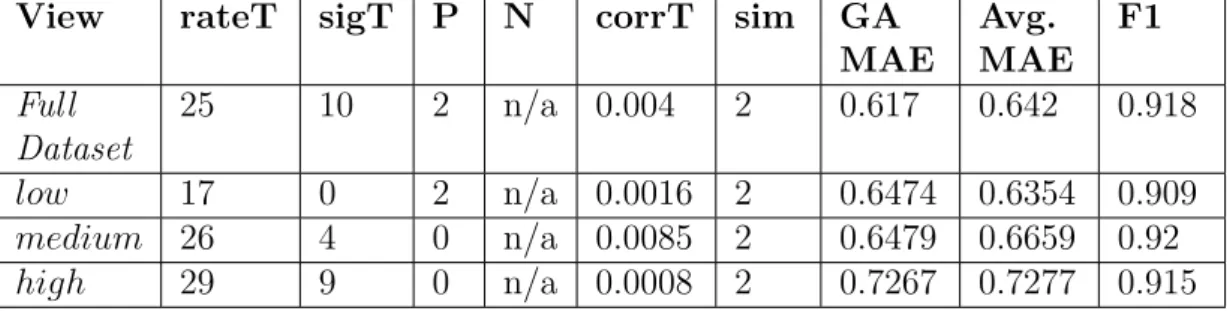
5.4 Results: User Rating Views . . . 70
5.5 Results: Popular Item Views . . . 74
5.6 Results: Comparing Evolved Parameters Across Views . . . 78
5.7 Discussion of Results . . . 80
5.8 Conclusions, Contributions and Future Work . . . 81
6 A Machine Learning-based Approach to Performance Predic-tion 83 6.1 Introduction . . . 83
6.2 Motivations . . . 84
6.3 Performance Prediction Approach . . . 85
6.3.1 Learning the Performance Prediction Rules . . . 85
6.3.1.1 Extract Rating Information . . . 86
6.3.1.2 Collaborative Filtering Technique . . . 88
6.3.1.3 Create Training and Test Tuples . . . 88
6.3.1.4 Machine Learning Technique . . . 89
6.4 Evaluation: Testing the Rules . . . 89
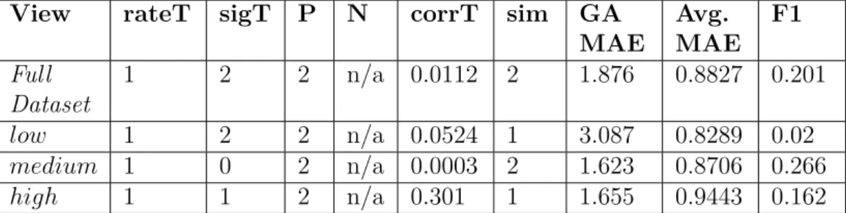
6.5 Results . . . 91
6.5.1 M ovieLens . . . 91
6.5.2 last.f m . . . 92
6.5.3 bookcrossing . . . 95
6.5.4 Epinions . . . 97
6.5.5 Performance Prediction Scenario . . . 98
6.6 Discussion of Results . . . 99
7 A Machine Learning-based Approach to Performance
Predic-tion with Dataset Views 101
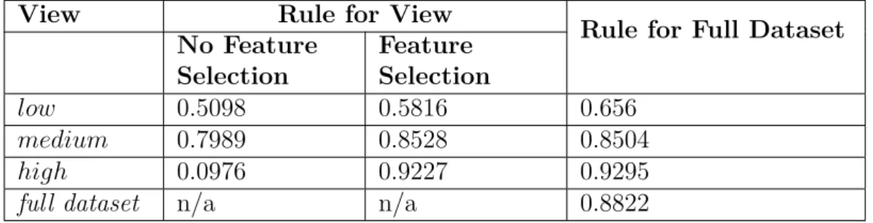
7.1 Introduction . . . 101 7.2 Motivations and Overview . . . 102 7.3 Methodology Review . . . 102 7.4 Results: Predicting Performance for the User Rating Views . . . 106 7.4.1 M ovieLens User Rating Views . . . 106 7.4.1.1 Best Performing Rule . . . 107 7.4.1.2 Rules with and without Feature Selection . . . 108 7.4.1.3 View Results versus Full Dataset Results . . . . 108 7.4.2 last.f m User Rating Views . . . 108 7.4.2.1 Best Performing Rule . . . 110 7.4.2.2 Rules with and without Feature Selection . . . 110 7.4.2.3 View Results versus Full Dataset Results . . . . 111 7.4.3 bookcrossing User Rating Views . . . 111 7.4.3.1 Best Performing Rule . . . 112 7.4.3.2 Rules with and without Feature Selection . . . 113 7.4.3.3 View Results versus Full Dataset Results . . . . 113 7.4.4 EpinionsUser Rating Views . . . 114 7.4.4.1 Best Performing Rule . . . 115 7.4.4.2 Rules with and without Feature Selection . . . 115 7.4.4.3 View Results versus Full Dataset Results . . . . 116 7.4.5 User Rating Views Summary . . . 117 7.5 Results: Predicting Performance for the Popular Item Views . . 117 7.5.1 M ovieLens Popular Item Views . . . 118 7.5.1.1 Best Performing Rule . . . 118 7.5.1.2 Rules with and without Feature Selection . . . 118 7.5.1.3 View Results versus Full Dataset Results . . . . 119 7.5.2 lastf.f m Popular Item Views . . . 119 7.5.2.1 Best Performing Rule . . . 120 7.5.2.2 Rules with and without Feature Selection . . . 120 7.5.2.3 View Results versus Full Dataset Results . . . . 120 7.5.3 bookcrossing Popular Item Views . . . 121 7.5.3.1 Best Performing Rule . . . 123 7.5.3.2 Rules with and without Feature Selection . . . 123 7.5.3.3 View Results versus Full Dataset Results . . . . 124 7.5.4 EpinionsPopular Item Views . . . 124 7.5.4.1 Best Performing Rule . . . 125 7.5.4.2 Rules with and without Feature Selection . . . 125 7.5.4.3 View Results versus Full Dataset Results . . . . 125 7.5.5 Popular Item Views Summary . . . 126 7.6 Discussion of Results . . . 127 7.7 Conclusions, Contributions and Future Work . . . 127
8 Conclusions and Future Work 129
8.1.3 bookcrossing . . . 133
8.1.4 Epinions . . . 133
8.2 Future Work . . . 133
8.3 Conclusion . . . 134
A Rules learnt for Datasets and Dataset Views 161 B Scatter Plots for Best Performing Rules for Dataset Views 173 B.1 Scatter Plots for M ovieLens Views: Best Performing Rules . . . 173
B.2 Scatter Plots for last.f m Views: Best Performing Rules . . . 176
B.3 Scatter Plots for bookcrossing Views: Best Performing Rules . . 179
B.4 Scatter Plots for EpinionsViews: Best Performing Rules . . . . 181 C Publications arising from the Work 185
List of Figures
3.1 Distribution of M ovieLens ratings. . . 33
3.2 Distribution of bookcrossing ratings. . . 34
3.3 Distribution of last.f m playcounts. . . 35
3.4 Distribution of log normalised last.f m playcounts. . . 36
3.5 Distribution of Epinions ratings: Number of Ratings by Users. . 37
4.1 Flow of control of GA experiment. . . 55
4.2 Average and best fitness of M ovieLens population at each gener-ation. . . 63
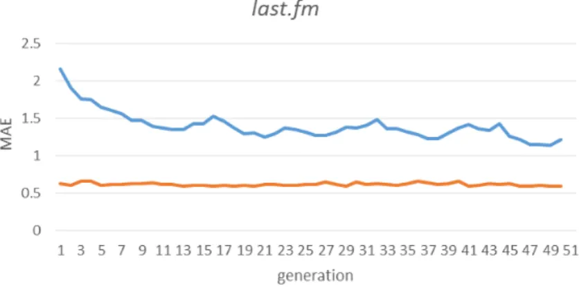
4.3 Average and best fitness of last.f m population at each generation. 63 4.4 Average and best fitness of bookcrossing population at each gen-eration. . . 63
4.5 Average and best fitness ofEpinionspopulation at each generation. 64 6.1 Performance prediction scenario in a collaborative filtering domain. 85 6.2 Steps to learn the performance prediction rules. . . 86
6.3 Steps to test the performance prediction rules. . . 90
6.4 M ovieLens predicted vs actual MAE values. . . 93
6.5 last.f m predicted (all features) vs actual MAE values. . . 94
6.6 last.f m predicted (with feature selection) vs actual MAE values. 95 6.7 bookcrossing predicted (all features) vs actual MAE values. . . 96
6.8 bookcrossingpredicted (with feature selection) vs actual MAE val-ues. . . 96
6.9 Epinionspredicted (all features) vs actual MAE values. . . 98
6.10 Epinionspredicted (with feature selection) vs actual MAE values. 98 B.1 M ovieLens low user rating view: Full Dataset Rule Scatter Plot. 173 B.2 M ovieLens medium user rating view: Full Dataset Rule Scatter Plot. . . 174
B.3 M ovieLens highuser rating view: Full Dataset Rule Scatter Plot. 174 B.4 M ovieLens low popular item view: Full Dataset Rule Scatter Plot. 174 B.5 M ovieLens medium popular item view: View Rule with All Fea-tures Scatter Plot. . . 175
B.6 M ovieLens highpopular item view: Full Dataset Rule Scatter Plot. 175 B.7 last.f m low user rating view: Full Dataset Rule Scatter Plot. . 176
B.8 last.f m medium user rating view: View Rule with Feature Selec-tion Scatter Plot. . . 176
B.9 last.f m high user rating view: View Rule with Feature Selection Scatter Plot. . . 177
B.10 last.f m low popular item view: Full Dataset Rule Scatter Plot. 177 B.11 last.f m mediumpopular item view: Full Dataset Rule Scatter Plot. 177 B.12 last.f m high popular item view: Full Dataset Rule Scatter Plot. 178 B.13 bookcrossing low user rating view: Full Dataset Rule Scatter Plot. 179 B.14 bookcrossing medium user rating view: View Rule with Feature Selection Scatter Plot. . . 179
B.16bookcrossing low popular item view: View Rule with All Features Scatter Plot. . . 180 B.17bookcrossing medium popular item view: View Rule Scatter Plot
(with and without feature selection the same). . . 180 B.18Epinions low user rating view: Full Dataset Rule Scatter Plot. . 181 B.19Epinions medium user rating view: View Rule with Feature
Se-lection Scatter Plot. . . 181 B.20Epinions highuser rating view: View Rule with All Features
Scat-ter Plot. . . 182 B.21Epinions low popular item views: Full Dataset Rule Scatter Plot. 182 B.22Epinions medium popular item views: View Rule with Feature
Selection Scatter Plot. . . 182 B.23Epinions high popular item views: Full Dataset Rule Scatter Plot. 183
List of Tables
3.1 Comparison of datasets used. . . 31
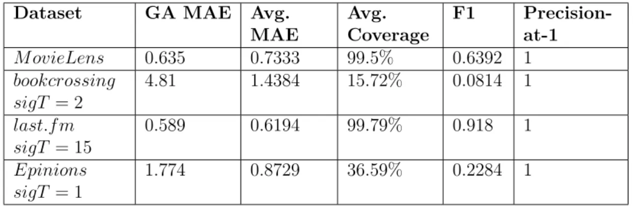
3.2 Comparison 1: Average MAEs and % Coverage for each dataset: Pearson Correlation Approach (10/90 Split). . . 38
3.3 Comparison 2: Average MAEs and % Coverage for theM ovieLens dataset with different test and train Splits: Pearson Correlation Approach. . . 39
3.4 Comparison 2: Average MAEs and % Coverage for the last.f m dataset with different test/train Splits: Pearson Correlation Ap-proach. . . 39
3.5 Comparison 2: Average MAEs and % Coverage for thebookcrossing dataset with different test and train Splits: Pearson Correlation Approach. . . 40
3.6 Comparison 2: Average MAEs and % Coverage for the Epinions dataset with different test and train Splits: Pearson Correlation Approach. . . 40
3.7 Average MAEs for each dataset with a number of techniques. . . 41
3.8 Comparison of Views: Massa et al. [160]. . . 43
3.9 Comparison of Views: Guo et al. [94]. . . 44
3.10 General Definition of Dataset Views . . . 45
3.11 Definitions of low,medium and high Dataset Views . . . 45
3.12 User Rating Views: M ovieLens. . . 46
3.13 User Rating Views: last.f m. . . 46
3.14 User Rating Views: bookcrossing. . . 46
3.15 User Rating Views: Epinions. . . 46
3.16 Popular Item Views: M ovieLens. . . 47
3.17 Popular Item Views: last.f m. . . 47
3.18 Popular Item Views: bookcrossing. . . 47
3.19 Popular Item Views: Epinions. . . 48
4.1 Values for Parameter P. . . 56
4.2 Experiment 1: Learning 4 parameters. . . 58
4.3 Experiment 1: Further Evaluation of Best set of GA Parameters. 59 4.4 Experiment 2: Learning 5 parameters. . . 60
4.5 Experiment 2: Evaluation of the Best set of GA Parameters. . . 61
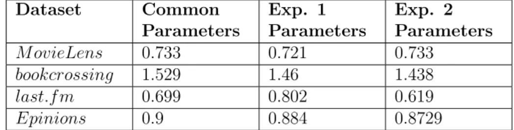
4.6 Comparing MAEs across Experiments. . . 62
5.1 The six parameters which will be evolved. . . 69
5.2 The GA Settings. . . 70
5.3 Learning parameters for the M ovieLens User Rating Views. . . 71
5.4 Comparison of MAEs: M ovieLens User Rating Views. . . 71
5.5 Learning parameters for the last.f m User Rating Views. . . 72
5.6 Comparison of MAEs: last.f m User Rating Views. . . 72
5.7 Learning parameters for the bookcrossing User Rating Views. . 73
5.11 Learning parameters for theM ovieLens Popular Item Views. . 75 5.12 Comparison of MAEs: M ovieLens Popular Item Views. . . 75 5.13 Learning parameters for thelast.f m Popular Item Views. . . 76 5.14 Comparison of MAEs: last.f m Popular Item Views. . . 76 5.15 Learning parameters for the bookcrossing Popular Item Views:
rateT held constant. . . 77 5.16 Comparison of MAEs: bookcrossing Popular Item Views. . . 77 5.17 Learning parameters for theEpinionsPopular Item Views: rateT
held constant. . . 78 5.18 Comparison of MAEs: Epinions Popular Item Views. . . 78 5.19 low User Rating View: Parameters for three Datasets. . . 79 5.20 medium User Rating View: Parameters for four Datasets. . . . 79 5.21 high User Rating View: Parameters for four Datasets. . . 79 5.22 Low Popular Item View: Parameters for four Datasets. . . 80 5.23 M edium Popular Item View: Parameters for four Datasets. . . . 80 5.24 High Popular Item View: Parameters for three Datasets. . . 80 6.1 Average MAEs for each dataset: Pearson Correlation Approach
(10/90 Split). . . 91 7.1 Features extracted per Dataset View. . . 103 7.2 Learning M ovieLens Features for User Rating Views: Pearson
Correlation comparison. . . 107 7.3 LearningM ovieLens Features for User Rating Views: MAE
com-parison. . . 107 7.4 LearningM ovieLensFeatures for User Rating Views: R2
compar-ison. . . 107 7.5 Learninglast.f m Features for User Rating Views: Pearson
Corre-lation comparison. . . 109 7.6 Learning last.f m Features for User Rating Views: MAE
compar-ison. . . 109 7.7 Learninglast.f m Features for User Rating Views: R2 comparison. 110 7.8 Learning bookcrossing Features for User Rating Views: Pearson
Correlation comparison. . . 113 7.9 LearningbookcrossingFeatures for User Rating Views: MAE
com-parison. . . 114 7.10 Learning bookcrossing Features for User Rating Views: R2
com-parison. . . 114 7.11 LearningEpinions Features for User Rating Views: Pearson
Cor-relation comparison. . . 116 7.12 Learning Epinions Features for User Rating Views: MAE
Com-parison. . . 116 7.13 LearningEpinionsFeatures for User Rating Views: R2 comparison. 117 7.14 Learning M ovieLens Features for Popular Item Views: Pearson
7.15 LearningM ovieLensFeatures for Popular Item Views: MAE
com-parison. . . 119
7.16 Learning M ovieLens Features for Popular Item Views: R2 com-parison. . . 120
7.17 Learning last.f m Features for Popular Item Views: Pearson Cor-relation comparison. . . 121
7.18 Learninglast.f mFeatures for Popular Item Views: MAE compar-ison. . . 121
7.19 Learninglast.f m Features for Popular Item Views: R2 comparison. 121 7.20 Learning bookcrossing Features for Popular Item Views: Pearson Correlation comparison. . . 122
7.21 Learning bookcrossing Features for Popular Item Views: MAE comparison. . . 122
7.22 Learning bookcrossing Features for Popular Item Views: R2 com-parison. . . 123
7.23 LearningEpinionsFeatures for Popular Item Views: Pearson Cor-relation comparison. . . 125
7.24 Learning Epinions Features for Popular Item Views: MAE com-parison. . . 126
7.25 Learning Epinions Features for Popular Item Views: R2 compar-ison. . . 126
A.1 M ovieLens Low Views . . . 162
A.2 M ovieLens Medium Views . . . 163
A.3 M ovieLens High Views . . . 164
A.4 last.f m Low Views . . . 165
A.5 last.f m Medium Views . . . 166
A.6 last.f m High Views . . . 167
A.7 bookcrossing Low Views . . . 168
A.8 bookcrossing Medium Views . . . 169
A.9 bookcrossing High Views . . . 169
A.10EpinionsLow Views . . . 170
A.11EpinionsMedium Views . . . 171
submitted for another degree, either at University College Cork or elsewhere. All external references and sources are clearly acknowledged and identified within the contents. I have read and understood the regulations of University College Cork concerning plagiarism.
Abstract
The work described in this thesis pertains to the area of Collaborative Filtering
and focuses on collaborative filtering datasets and specially-defined portions of the datasets called views. The high level goal of the work is to better
understand how different characteristics of datasets affects the performance of collaborative filtering techniques. Datasets, and views, are compared across a number of different experiments: some relating to techniques and accuracy and others relating to ideas of performance prediction.
Acknowledgements
With thanks to:
• Humphrey Sorensen for support, guidance, help and belief. • Colm O’Riordan for proof-reading and advising.
• the external examiner, Prof. Tommaso Di Noia, Politecnico di Bari, Italy. • the internal examiner, Adrian P. O’Riordan, University College Cork. • staff in University College Cork who have facilitated this journey. • the National University of Ireland, Galway for support and financial
assistance.
• the many reviewers for helpful comments and reviews of papers resulting from this work.
• the research groups and people who made datasets freely available directly or via their APIs (in particular GroupLens, last.f m, bookcrossing and Epinions).
• my colleagues and friends in NUI Galway for help, support and patience. • family and friends for being.
Introduction and Overview
1.1
Motivations
Modern information spaces have become more complex where information and users are linked in numerous ways, both explicitly and implicitly, and where users are no longer anonymous, but generally have some identification and a context in which they navigate, search, browse and seek recommendations. This offers new challenges to information retrieval system designers, both in capturing this information and using it to provide for a more personalised and effective retrieval and recommendation experience for a user.
Collaborative filtering provides one approach to recommendation. Generally, col-laborative filtering techniques make use of one type of information, that is, prior implicit or explicit ratings that users have given to items. The assumption upon which collaborative filtering is based is that human preferences are correlated and thus prediction of future preferences is possible. Specifically, given a set of ratings by users for items, the aim of collaborative filtering is to predict the ratings of a particular user, u, for one or more items, i, previously not rated by that user. The traditional, and prevalent, recommendation paradigm involves a centralised approach whereby users register with one particular system and provide ratings for items (explicitly, implicitly or both) and receive recommendations on new unseen items.
This chapter will give an overview of the research problems which will be ad-dressed by the work described in this thesis (Section 1.2). The aims of the work (Section 1.3) and the research challenges that will be addressed are then outlined
(Section 1.4). The main methodology used (Section 1.5) and the contributions of the work (Section 1.6) are outlined in the subsequent sections. Finally, an overview of the topics discussed in each subsequent chapter is given (Section 1.7).
1.2
Open Research Problems
The 1990s saw the first set of publications in the area of collaborative filtering, although many of the techniques on which the work was based were well-known from the statistics and information retrieval domains. Work by Goldberg et al. [82] and Shardanand and Maes [214] introduced the problem domain and the idea of leveraging user preferences to make recommendations. It was unlikely that these early pioneers of the area envisaged that, in the space of 20 years, collaborative filtering techniques would be in widespread use and that a very large number of models would have been proposed and evaluated.
The focus of the publications in the intervening years has been naturally diverse but some main themes and problems have remained relatively constant. Some of the most-studied aspects of the domain have been concerned with improv-ing the accuracy of recommendations and improvimprov-ing user satisfaction with the recommendations and with the recommender systems.
The aspects of the domain which this work seeks to address include:
1. The majority of previous research is evaluated using standard, freely-available datasets and it is generally recognised that techniques will have different performances given the particular dataset under study. In much of the work the analysis of the techniques have predominated, with very little attention given to the characteristics of the datasets and how these characteristics vary across datasets.
2. There is much evidence from various domains within Information Retrieval and Recommender System research that there are many factors which can contribute to effective retrieval and recommendation. Much of the previous work has focused on developing and evaluating new collaborative filtering techniques, with the focus predominately on increasing accuracy. Despite the wealth of research done in this area there remains fruitful avenues for further research. One such avenue relates to how different algorithms, and parameter value settings of the same algorithm, might give better or worse
performance depending on the dataset used.
3. Some well-known collaborative filtering problems exist with respect to the sparsity of the datasets, where typically users only rate a small number of items and many items receive few or no ratings. Many of the previous models developed try to overcome this problem with different approaches. However the characteristics of the datasets has generally not been leveraged to explain why particular users may not receive good recommendations. 4. Features of collaborative filtering datasets (such as a user’s average rating
value and standard deviation from this average) have been used in many of the techniques developed. However, such features have rarely been used to predict how well an approach might perform given the features of some user or some item.
1.3
Aims
Given the four issues identified in the previous section, the high-level aims of this work are toidentifyand analysethe information which can be extracted, compared and learned across collaborative filtering datasets, and portions of
these datasets. The aim is not only to show that improved accuracy can be
obtained in certain cases, but to better understand why such accuracy may or may not be achieved. In addition the aim is to examine whether — given the user, dataset or portion of dataset, in question — the accuracy can bepredicted
in advance of recommendation.
1.4
Research Challenges
The focus of this work lies in the areas of collaborative filtering, collaborative filtering datasets, collaborative filtering parameters (for a memory-based near-est neighbour approach) and performance prediction. There are four research challenges identified in these areas:
C1: How to analyse and compare characteristics of different datasets.
C2: How to find the best set of parameters in a nearest neighbourhood approach for different datasets and portions of datasets.
C3: How to understand, in some way, why particular recommendations for a user may or may not be accurate.
C4: How to provide a measure of the system’s confidence in the recommenda-tions given.
The hypotheses are:
H1: Comparison: A comparison between collaborative filtering datasets can be used to explain the recommendation accuracy likely to be achieved when using the datasets. (Challenge C1).
H2: Learning Parameters: A genetic algorithm approach can be used to find the best set of parameters for different collaborative filtering datasets. (Chal-lenge C2).
H3: Predicting Performance: A set of features can be extracted from the datasets and can be used to predict the performance of a recommender system for a particular user. (Challenges C3 and C4).
1.5
Methodology
The methodology is based on standard collaborative filtering techniques, partic-ularly a Pearson correlation nearest-neighbour approach. The evaluation metrics used are predominantly mean absolute error (MAE) and coverage, but also the F1 metric. The machine learning techniques of genetic algorithms and an ID3 decision tree are also used. Four datasets are considered in each experiment: M ovieLens,last.f m,bookcrossing and Epinions.
1.6
Contributions
The work makes the following contributions:
1. Specifying the information which can be captured in collaborative datasets to aid comparison across datasets. (See Chapter 3). (Relating to Hypothesis 1 [H1]). (Published [86, 87]).
2. Extracting feature and “view” information from a number of different datasets and comparing the features and views across the datasets. (See all chapters). (Relating to Hypothesis 1 [H1]). (Published [88, 89]).
3. Using a genetic algorithm to learn the best set of features per dataset in a nearest-neighbour approach (See Chapter 4 and Chapter 5). (Relating to Hypothesis 2 [H2]). (Published [90]).
4. Providing a measure of confidence in the predictive accuracy of a recom-mender system prior to recommendation. (See Chapter 6 and Chapter 7). (Relating to Hypothesis 3 [H3]). (Published [91, 92]).
1.7
Thesis Overview
Chapter 2 presents an overview of the aspects of collaborative filtering areas that are most relevant to the work described in this thesis. Chapter 3 provides a general discussion of collaborative filtering datasets — their characteristics and an outline of some of the main studies where they have previously been used. This is followed by a detailed discussion and comparison of the four datasets used in this work. Finally, specially-defined portions of the four datasets, called
dataset views, are defined and analysed. Chapter 4 outlines a genetic algorithm
approach to learn the best set of values for common parameters in a nearest-neighbour Pearson correlation approach. Chapter 5 continues this work but con-siders the genetic algorithm approach applied to the previously-defined dataset views. Chapter 6 outlines a performance prediction approach to enable a level of predictive accuracy which could be made available to users prior to recommenda-tion. The learning approach is based on dataset features which are extracted from the datasets prior to a learning stage (using decision trees). Chapter 7 returns again to dataset views, and outlines the results obtained when the performance prediction approach, outlined in Chapter 6, is applied to dataset views. Chapter 8 concludes the thesis with a summary of the work done, the main contributions of the work and with a list of some ideas for future, related work.
The Case for Collaborative
Filtering
The Models, Techniques, Successes and Challenges
2.1
Introduction
The goal of this chapter is to present an overview of current knowledge in the many inter-related areas of collaborative filtering relevant to the research work outlined in this thesis. The layout of the chapter is built upon a generic model of the main components of a collaborative filtering system. Much of the focus centres on the approaches that are used for the prediction of recommendations. Another major focus is on the approaches used to evaluate the collaborative filtering results.
The outline of the chapter is as follows: firstly a brief overview is given of the dif-ferent motivations for collaborative filtering research. The area of collaborative filtering is then described through the use of a model which lists five compo-nents: Users, Items, Datasets, Models and Recommendations. The components of U sers, Itemsand Datasetsare first explored in Section 2.4, although most of the discussion of datasets is deferred to the next chapter (Chapter 3). Section 2.5 contains a discussion of the many collaborative filtering models which have been proposed. The discussion centres on three main models: memory-based models; graph-based models and probabilistic models. In addition, three extensions of these models — in the form of combination approaches, weighting schemes and
learning approaches— are discussed in separate sub-sections. Finally, Section 2.6
concentrates on issues surrounding the evaluation of the recommended items re-turned by a collaborative filtering approach. In addition to a predictive-accuracy focus and a user-centric focus, some work which considers explanations and pre-dictive performance is discussed. Conclusions are presented in Section 2.7.
2.2
Motivations of Collaborative Filtering
Re-search
The original foundations of collaborative filtering emerged from the idea of “au-tomating the word of mouth process” that commonly occurs within social net-works [214], i.e., people will seek recommendations on books, CDs, restaurants, etc., from people with whom they share similar preferences in these areas. Given a set of users, a set of items, and a set of ratings, collaborative filtering sys-tems attempt to recommend isys-tems to users based on user ratings. Collaborative filtering systems traditionally make use of one type of information, that is, prior explicit or implicit ratings that users have given to items. The incorporation of additional information, particularly content and explicit social information, has also been considered. To date, application domains have predominantly been con-cerned with recommending items for sale (e.g., movies, books, music and accom-modation) and with small amounts of text such as review articles and bookmarks to websites. The datasets within different domains have their own characteristics, but they can be predominantly distinguished by the fact that they are both large and sparse, i.e., in a typical domain, there are many users and many items but any user will only have given ratings to a small percentage of all items in the dataset.
For convenience, the problem space is often viewed as a matrix consisting of the ratings given by each user for the items in a collection, i.e., the matrix consists of a set of ratings ra,i, corresponding to the rating given by a user a to an item
i. Using this matrix, the aim of collaborative filtering is to predict the ratings of a particular user, a, for one or more items not previously rated by that user. The problem space can alternatively be viewed as a graph where nodes represent users and items, and nodes and items can be linked by weighted edges in various ways. Graph-based representations have been used for both recommendation and social network analysis of collaborative filtering datasets [115, 192, 55].
Many different approaches to the collaborative filtering task have been investi-gated, each with their own set of assumptions with respect to the collaborative fil-tering dataset. Studies have different foci — usually, but not only, to improve pre-dictive performance. Other issues of interest include: scalability [206, 78, 29, 135, 76, 147, 8, 251]; dealing with sparseness [181, 151, 152, 186, 45, 111]; including ad-ditional information [239, 61, 183, 50]; trustworthiness [162, 123, 240, 73]; novelty [252, 173, 247, 199], transparency and explanation [103, 168, 158, 132, 107, 207] and predicting performance [188, 69, 27].
Similar to software quality in general, and information retrieval system quality specifically, measures of collaborative filtering quality are typically linked to a system’s superiority (or non inferiority) in meeting a set of requirements with
respect to one or more metrics. These measures have important consequences in that the relative merits of systems and algorithms can be compared empirically and assurances of quality with respect to these metrics can be associated with systems and algorithms.
2.3
Collaborative Filtering: An Overview
The collaborative filtering task can be viewed as a typical prediction problem, i.e., for some user, and some past evidence of the user’s, and other user’s, interests, predict the user’s interest for some unseen items.
A general model for collaborative filtering can be defined, based on a similar model in Information Retrieval [11], by:
< U, I, P, M, R(I, u)> where:
• U is a set of users, generally represented by some unique identifier although additional demographic information on users may exist.
• I is a set of items (dependent on the domain) generally represented by some unique identifier; again, additional information on items may exist.
• P is the dataset (i.e., can be viewed as a matrix of dimension |U| × |I|
containing ratings by users U for items I where a value in the matrix is referenced by pui);
• M is the collaborative filtering model(s) used (e.g., correlation methods; probabilistic models; machine learning approaches); and
• R(I, u) returns a set of recommended items fromI (which may be ranked) based on P and M, given user u.
A possible instantiation of the above framework within a movie recommender domain (the M ovieLens100K dataset1) can be specified as follows:
• U consists of a set of 943 users, represented by unique IDs, seeking recom-mendations on movies.
• I consists of a set of 1682 items (which are movies), represented by a unique identifier for each movie.
• P is the collaborative filtering dataset,M ovieLens100K, containing ratings by the users U for items I. A rating is an integer value in the range [1−5]
indicating a user’s preference value for a movie, from 1, indicating a user does not like the movie, to 5, indicating that a user loves a movie. The M ovieLens100K dataset contains 100,000 ratings.
• M is the model or models used. There exist many possible instantiations ofM. One common approach is to calculate the similarity between users in U based on the correlation of the ratings they have given to itemsI. These similarity values are used to select neighbours and calculate a recommen-dation value for items.
• Based on the output of the modelM,R(I, u) returns a ranking of some, or all, of the items in I which user uhas not previously rated.
2.4
U
: The Users;
I
: The Items and
P
: The
Dataset
In collaborative filtering domains, users give ratings to items and these ratings become the main input to a collaborative filtering model. The ratings may be in a restricted range, or not, and may be gathered explicitly (for example a star rating from 1 to 5 for an item) or implicitly (for example the number of times an item was accessed).
Although traditionally a dataset consisted only of the ratings by users for items, there are more dimensions to these basic components in some modern datasets, e.g.,
• content information on the users may be stored and used, for example demographic information or profile information.
• explicit link information between users may be stored, for example trust links or friendship links.
• content information on the items may be stored and used, for example attributes of items, tags associated with items or descriptions or reviews of items.
• a time stamp may be associated with the ratings.
Typically, there are many users and many items in any system and a predominant feature of collaborative filtering datasets is that they are both large and sparse. Some approaches deal specifically with sparseness [157], including work to esti-mate and fill missing data: Rao et al. take advantage of additional information that is available on users and use a low rank matrix completion approach [191];
Hu et al. and Xue et al. use smoothing approaches [113, 238] and George et al. [78] and Li et al. [150] use a co-clustering algorithm. Kim et al. develop a binomial mixture model where the model jointly handles non-random missing data as well as generating predictions [129].
The large size of the datasets often results in poor performance. Singular Value Decomposition (SVD) has been used to improve scalability by dimensionality reduction [33, 206, 16]. Latent factorization techniques have proved to be far more scalable than other approaches with large datasets [194, 218, 220, 216, 53, 30, 106, 156].
One common characteristic of collaborative filtering datasets seen in earlier work was called the “cold start” problem and has, in more recent work, been termed the “long tail” of item distribution within the datasets [10]. This refers to items which have not received many ratings or users who have not given many ratings. This may be due to the fact that the users or items are newly introduced to the dataset or, for items, it may be that the items are unpopular or that they are niche items. Many studies remove these items from the datasets or modify models and algorithms to deal with them [209, 114, 131], while other studies attempt to gather more ratings [249, 5, 51] or attempt to gain some benefit from the existence of the long tail distribution [212, 182].
Some of the previous work in this area builds on theoretical and mathematical work on high dimensional spaces and distance measures in the areas of database
systems [31, 2, 74, 190]. One such result showed that “in high dimensional space, the concept of proximity, distance, or nearest neighbour may not even be quali-tatively meaningful” [2], i.e. in high dimensional data distances between all pairs of points become almost equal.
Recent work by Aharon et al. [5], in an online setting, use a matrix factorization approach to find users with distinctive tastes who can give feedback (ratings) on new items. Zhou et al. [249] develop an approach which can be used to elicit user preferences by having users answer some set of adaptive questions. They use a functional matrix factorization approach to build a decision tree where each node in the tree corresponds to a question. Chang et al. [51] also develop an approach for rating elicitation where users are asked to give a rating to a cluster of similar items, rather than a single item. Ling et al. [154] use a matrix factorization approach to combine content and collaborative information; while Saveski et al. [207] use a similar approach but use the similarity between users and between items in their matrix factorization approach. Fernandez-Tobias et al. [72] compare a number of different algorithms using rating data and content data extracted from DBpedia2.
2.5
M
: The Collaborative Filtering Models
A large body of work has concentrated on different collaborative filtering models (M) and their evaluation and comparison. An overview of three families of col-laborative filtering models will be given here: memory-based models; graph-based models; and probabilistic models (including matrix factorization techniques). Three further sub-sections will discuss variations of these models: one involv-ing the combination of models and/or data; the second involvinvolv-ing the effect of the modification of the value of parameters in some of the models and finally, the third, presenting studies which have sought to learn, using genetic algorithms, the best model, or models and weighting schemes, to use.
2.5.1
Memory-based Models
The most popular and successful early approach to collaborative filtering was that of a group of techniques which belong to what is termed “memory-based”
approaches — which are also called neighbourhood-based approaches. The typical neighbourhood-based approach uses standard measures to calculate the similarity between users (for example, mean square difference, Pearson correlation, cosine similarity etc.) to find a user’s neighbours. Much early work empirically evaluated variants of the approach [39]. Herlocker et al. tested a classic neighbourhood-based collaborative filtering algorithm [104]. A number of similarity measures were used to find neighbours, with a significance threshold used to dampen the similarity for users who had only rated a few items, choosing the k most similar users as neighbours for prediction and using “deviation from the mean” as the normalisation method. The components tested included:
• the size of the neighbourhood used.
• the similarity measure used to compute the closeness of neighbours. • the threshold over which other users were considered neighbours. • the type of normalisation used on the ratings.
The standard M ovieLens100K dataset was used comprising 100,000 movie rat-ings from 943 users on 1682 items and the mean absolute error metric (MAE) was used to compare results. The overall observations from the work for the M ovieLens dataset were [104]:
• Use Pearson correlation for the similarity measure.
• Dampen similarity scores between users who have co-rated a small number of items. A devaluation term above 50 did not appear to improve results. The devaluation term was used by multiplying two user’s correlation by n d
wheren is the number of co-rated items between the two users and dis the devaluation value.
• Normalize user ratings by “deviation from the mean” to account for user’s rating with slightly different scales, i.e., each user rating is taken as their raw rating score minus their mean score.
• Use theT opN best neighbours (highest similarity to the test user) for neigh-bourhood selection. The estimated best range of neighbours (N) was found to be between 20 and 60.
• Weight neighbour contributions when forming predictions.
Although the approach outlined by Herlocker et al. [104], and the parameters used, offered good performance, Howe et al. [112] re-evaluated two parameters
from Herlocker et al.’s work — the similarity measure between users and the normalisation of user ratings — using the M ovieLens and Netflix dataset, and found that Pearson correlation is not necessarily the best similarity metric to use. They compared cosine vector similarity, Pearson correlation, Spearman cor-relation, Manhattan distance, Euclidean distance, L∞ distance and Hamming
distance. They found that different parameterisations work better for different datasets.
2.5.2
Graph Models
Several researchers have adopted graph representations to develop recommenda-tion algorithms. A variety of graphs have been used, including, directed and two-layered graphs. A number of graph algorithm approaches have been adopted [3, 115, 96, 137] with recent work focusing on random walk algorithms that rank vertices (where vertices represent items) [148, 57, 55]. The graph approach has also been used to integrate sources of evidence and information [239, 61] including information from social networks [73, 50].
A number of recommender systems based on social networks have been devel-oped3. Early work induced these social networks from the rating data (for exam-ple, the common items that users have rated [15, 180, 192]) and by matching user models and profiles [230]. Recently, online relationships between people have been used to create social networks and many examples of explicit social networks exist where relationships between users are explicitly created and where there is con-tent (comments, images, movies) associated with the users in the social network [136, 50].
2.5.3
Probabilistic Models
Probability theory has been used in many collaborative filtering approaches [184, 222, 136]. Many of the probabilistic algorithms construct a model of underlying user preferences from which predictions are inferred. Examples include Bayesian models [39, 246, 14]; dependency networks [101], social networks [50], aspect models [108, 109, 97], expectation maximization models [141], clustering models
3A social network can be defined as a network (or graph) of social entities (e.g. people, markets, organisations, countries), where the links (or edges) between the entities represent social relationships and interactions (e.g. friendships, work collaborations, social
[228, 28, 1] and models of how people rate items [184]. Other machine learning approaches have been considered [17, 33, 174, 75], including deep neural networks [58], as well as approaches which view the problem as a list-ranking problem [75, 155], a multi-objective optimisation problem [179] and as a data mining problem [3, 172].
Based on a probabilistic framework, matrix factorization techniques have become one of the new standards in collaborative filtering research when dealing with very large datasets and when scalability is an issue [233, 138, 187, 18, 53, 30, 106, 156, 100, 128]. In general, the idea of a matrix factorization approach is to factor the rating matrix into two sub-matrices: one related to items and one related to users [135]. The factorization approach is based on finding K latent factors that allow prediction of items for some user. The approach is often instantiated as an optimisation problem. Once the optimisation problem is solved, one vector represents the user (~a) and the second vector represents the item (~b) on which the user will receive a prediction. Each vector has K factors. The prediction for a user u for item iis: Pu,i =a~u×b~i.
Steck [216] extends a matrix factorization technique by the use of non-linear ac-tivation functions (often found in neural networks). The model is tailored to sparse binary data using a binary version of the M ovieLens10M and N etf lix datasets. Hernando et al. [106] improve upon a classical matrix factorization ap-proach using a Bayesian probabilistic model for non-negative matrix factorization. Their approach provides a way to understand why particular recommendations were made — which is generally difficult to provide with a matrix factorization approach.
Liu at al. [156] combine a matrix factorization approach with kernel methods and multiple kernel learning. They show that their approach captures non-linear correlations among data which in turn leads to improved accuracy in comparison to five other techniques. They evaluated the approach on six datasets (three of which wereM ovieLens,J ester and F lixster). The techniques used for compar-ison to the one-kernel and multiple-kernel matrix factorization approaches were three memory-based approaches (baseline average, item-based cosine similarity, item-based Pearson similarity) and two model-based approaches (Singular Value Decomposition (SVD) and a baseline matrix factorization approach). RMSE was used as the metric for comparison. Results indicated that the one-kernel and multiple-kernel matrix factorization approaches outperformed the other baseline approaches.
2.5.4
Combination
There is much evidence from various domains within Information Retrieval that the combination of sources of evidence leads to more effective retrieval [62]. With respect to recommender systems, Basu et al. claim that “there are many factors which may influence a person in making choices, and ideally, one would like to model as many of these factors as possible in a recommendation system” [17]. Although the types of information combined, and the techniques used, vary sub-stantially across the domains, it has been shown that there are advantages to be gained from considering more than one source of information or more than one technique.
There are two main approaches in collaborative filtering combination: the first approach involves using two or more techniques for each type of data present and combining/blending the prediction scores of each approach to get a final prediction score for each recommended item [12, 178, 46, 135, 215, 119, 221, 154]. The second approach involves extracting, or using, additional information (or features) from the collaborative filtering dataset and incorporating this into the collaborative filtering approach [180, 175, 204, 231, 113, 198, 183, 67, 136, 50]. In terms of the first approach, the Netflix competition demonstrated that, rather than a new technique, it was the combination, or blending, of existing techniques, which resulted in substantial improvements in accuracy [29]. The work demon-strated that latent factor models, such as matrix factorization, provide better accuracy, deal with sparsity and large datasets better, provide good scalability and allow for the incorporation of additional information [135, 76]. Jahrer et al. [119] further strengthen the argument for a combination of models in their work where they analyse 18 different algorithms and show that linearly combining a set of algorithms outperforms any single algorithm. In terms of the second approach, some work combined, in addition to ratings, context information [198], content information [183, 67] or both context and content information [126]. Recent stud-ies have combined different types of data. Examples include the work by Kouki et al. [136] where user-user, item-item and social information are incorporated into their recommender system using a hinge-loss markov random field approach [136]. Chaney et al. use a probabilistic matrix factorization approach to combine social information with rating information [50].
2.5.5
Weighting Schemes
A complementary approach to improving performance by the use of one or more models M involves the investigation of weighting schemes for collaborative filter-ing where these weightfilter-ing schemes typically try to model some underlyfilter-ing bias or feature of the dataset in order to improve prediction accuracy. For example, early work by Breese et al. [39] and Yu et al. [244] apply an inverse user frequency weighting to all ratings where items that are rated frequently by many users are penalised by giving the items a lower weight. Similarly, variance weightings have been used to increase the influence of items with high variance and decreased the influence of items with low variance [102, 244]. The idea of a tf-idfweighting
scheme from information retrieval has been used for a (matrix) row normalisation [127] and as part of a probabilistic framework [231]. Machine learning approaches have been used to learn the optimal weights to assign to items [54, 124, 192]. O’ Donovan et al. give a higher weighting to user neighbours that have provided good recommendations in the past [176]. DeBruyn et al. give items which are recommended more frequently a higher weighting [66].
In general, although the use of some of the weighting schemes for items has shown improved prediction accuracy (in particular those involving learning), it has proved difficult to leverage the biases in the datasets to consistently improve results. There may be a number of reasons for this, including the fact that the datasets are sparse and that the data may not always be correct. Even if the data is correct, the underlying preferences that the data “describes” may not always be consistent, as user tastes and opinions may change over time [142, 42, 235, 232]. Related to the modelling of some underlying bias or features of the dataset in order to improve prediction accuracy is the work done on analysing the models to give an indication as to which models are more resilient to malicious attacks (e.g., “shilling attacks” where ratings are entered into the system to bias results) [248, 169, 140, 43, 177, 211]. Another related issue is that of trust. O’Donovan and Smyth [176] state that “profile similarity on its own may not be sufficient”. They, and others, incorporate trust measures into standard approaches using both implicit and explicit measures of trust [162, 7, 117, 226, 120, 121, 38, 123, 73]. Yang et al. [240] fuse rating data and trust data by mapping users into two low-dimensional spaces, i.e.,trusterspace andtrusteespace, using matrix factorization
techniques. Forsati et al. [73] also use a matrix factorization technique and incorporate information ontrustanddistrustinto theirPushTrustmodel. Results
other baseline matrix factorization approaches. In addition, it was shown that
distrust is beneficial for the recommendation process.
2.5.6
Learning
Given the many models that have been proposed, and the many variations that exist within these models, some work has applied the evolutionary learning ap-proach of genetic algorithms4 to choose the best models, or combinations of mod-els, or to choose the best set of weights or parameter values for a particular technique. Ujjin et al. [227] use a genetic algorithm to find the best “profile” that describes each user in the dataset. Ko et al. [133] first classify items into groups using a Bayesian classifier to reduce the dimensions of the space. A genetic algorithm is used to cluster users in the new lower dimensional space. Hwang et al. use a genetic algorithm, per user, to learn an optimal weighting scheme for the collaborative filtering system for each user [116, 118].
Bobadilla et al. [34] use a genetic algorithm to find the best similarity function between vectors representing user’s ratings for items. The fitness function used is the Mean Absolute Error (MAE). They use three datasets (M ovieLens,N etf lix,
FilmAffinity). Results show that recommendations were returned more quickly,
and were of better quality, than the recommendations computed using traditional collaborative filtering approaches.
2.6
R
(
I, u
)
: Recommended Items
Irrespective of the approach used, the ability of a system to provide quality
rec-ommendations, R(I, u), is the main measure of effectiveness used in collaborative filtering systems. Intermediate steps within a particular approach can also be evaluated. Most experiments have been performed offline with a predictive ac-curacy focus but some recent work has incorporated online user-centric studies [213, 199, 70, 98].
In this section four aspects of recommender system evaluation will be considered. Firstly, the standard approach of offline predictive accuracy evaluation will be presented. User-centric evaluation will then be discussed. Finally two related
4Genetic algorithms are stochastic search techniques that evaluate a population of solutions (individuals) over a number of iterations (generations) and at each iteration, evaluate how good (or fit) each solution is [110, 81].
areas will be presented: offering an explanation of why recommendations were made; and using predictive techniques to improve the quality of the recommen-dations made.
2.6.1
Predictive Accuracy Focus
A number of studies have been carried out in order to compare, from a predictive accuracy perspective, the quality of the recommendations produced by various collaborative filtering algorithms. This generally involves one of two evaluation approaches: an error-based approach and an approach which evaluates a top-N
list of ranked recommendations.
It is important to note that only studies using the same datasets and the same evaluation approach can be meaningfully compared. As typically there are many parameters in different methods and evaluation approaches, we often cannot be fully confident that the comparisons across different studies are fully valid. Generally most experiments adopt the same testing methodology of decomposing a known collection of ratings by users over a range of items into two disjoint subsets. The first set (the training set, and usually the larger) is used to generate recommendations for items corresponding to those in the smaller set (the test or ground truth set). The generated recommendations are then compared in some way to the actual ratings in the test set.
Many of the datasets to date do not have a test and train portion and so it is left to individual experiments to decide on how to decompose the dataset. The main variability is in the size of the training and test set. Approaches include different percentile splits, (e.g., 10:90; 20:80; etc.) or a leave-one-out approach where recommendation is sought on only one item. Each different split will typically impact the error measurement. Many recent studies use a 5-fold cross validation approach. With this approach, users are partitioned into five sets. For each user in each set, 20% of the user’s ratings are randomly chosen as thetestratings. The
remaining ratings, in addition to all the ratings in the other partitions, become the training ratings.
2.6.1.1 Error-based Approaches
In most work, error-based approaches are used to measure the ability of the system to provide a recommendation on a given item (coverage) and to measure
the correctness of the recommendation generated for a given item by the system (accuracy). Specifically:
• coverage is a measure of the ability of the system to provide a
recommen-dation on a given item.
• accuracyis a measure of the correctness of the recommendations generated
by the system.
Coverage is usually computed as a percentage of the items for which the system is able to provide a recommendation. The most commonly used accuracy metrics include mean absolute error (MAE), normalised MAE (NMAE), and root mean square error (RMSE) — all of which compare the exact rating value given to an item by a user to the exact value predicted for the item by the system. The closer the two values are, the lower the error.
The MAE score is defined as:
PN
i=1|(pi−ri)|
N (2.1)
where forN test items on which the system returns predictions,pi is the predicted
rating for itemifrom the collaborative filtering system andri is the actual rating
given by a user to item i.
For several of the metrics there are two variants: overall and per-user; withoverall error, the overall error of all predictions for all users is averaged together; with per-user error the error per user is averaged first, and then all user averages
are subsequently averaged. Schein et al. found that averaging errors overall or per-user can give conflicting results [209]. Correlation measures between ratings
and predictions can also be used. Sarwar et al. claim that correlation measures and metrics such as MAE, RMSE, and NMAE track each other closely [205]. Work by Zhang et al. concentrates on reducing the complexity of the evaluation calculations [245].
Said et al. [197] compare results across three common recommender frameworks and find that, when using the same algorithms, RMSE values can differ by more than 10% across frameworks. They use the study to motivate the need for con-trolled evaluation across studies.
There has been criticism of the error-based approach, focussing on two main beliefs: that the recommendations which have the least error are not necessarily
the most useful [167]; and that a ranked list of recommendations (e.g. 1, top-5) more fully reflects the real-world usage of recommender systems where items are recommended but their predicted value is not important [60].
2.6.1.2 Top-N Approaches
Top-N approaches aim to measure coverage and accuracy by adopting the In-formation Retrieval metrics of precision and recall. Top-N approaches are the standard evaluation approach in Information Retrieval but there are many dif-ferences between Information Retrieval and collaborative filtering experimental settings. One of the largest differences is in the definition of item relevance, as this can only be defined per user, whereas in the information retrieval experimental setting, relevance can be taken as a ground-truth for all queries in a collection. To evaluate the top-N recommendations, Sarwar et al. [205] use modified versions of precision, recall and F1 metrics where items are divided into two sets — test set and top-N set. Items that appear in both sets are members of the hit set.
Recall is defined as (size of hit set
size of test set) and precision is defined as (
size of hit set size of top N set).
The F1 measure is then defined as usual as: (2×precision×recall precision+recall ).
Cremonesi et al. [60] present work that highlights approaches which perform well when evaluated with an RMSE metric but do not perform similarly with a top-N evaluation. They compare item-based neighbour models with latent factor models using the M ovieLens and N etf lix datasets. They note some problems with a top-N approach, notably that the most popular items in a dataset can bias the precision and recall results. This was also noted by Celma et al. [48] with the last.f m dataset. Cremonesi et al. overcame this bias by removing the very popular items from the dataset [60].
Bellogín et al. [26] state that there is variability in the way top-N evaluation methodologies are carried out and that this means results are not comparable across different studies. The biggest variability relates to what they refer to as the “amount of unknown relevance that is added to the test set”. That is, the many user-item pairings that have no rating and are often assumed, in the absence of any other knowledge, to not be relevant. They compare five test-ing methodologies with three collaborative filtertest-ing approaches (user-based and item-based neighbourhood approaches and a matrix factorization approach) and three different metrics (Precision, Recall and Normalized Discounted Cumulative Gain).
Herlocker et al. [105] give a comprehensive overview of testing and evaluation methodologies. They compare a large number of evaluation metrics including: mean absolute error, Pearson correlation, Spearman rank correlation, area under-neath a ROC-4 and ROC-5 curve, half life utility metric, mean average precision at relevant documents and NDPM (normalized distance-based performance mea-sure) metric. One of their contributions was to show that, for a given dataset, some metrics may be strongly correlated while other classes of metrics are un-correlated. They argued the case for recommender systems not only focusing on accuracy but also on usefulness in terms of coverage, learning rate, serendipity,
novelty and confidence. In addition they discussed metrics which can only be measured by user evaluation of recommender systems.
2.6.2
User-Centric Focus
Studies have shown that the most accurate recommendations are not necessarily the most useful from a user perspective [252, 167, 158]. For example, Bollen et al. [37] show that large sets of good (accurate) recommendations do not necessarily result in higher user satisfaction. Many authors claim that the focus on predictive accuracy, as a measure of recommender system quality, has been detrimental to the field [167, 199, 132].
User-centric studies have focused on including explanations [224, 158]; generating a more diverse (serendipitous) list of recommendations [252, 77, 143]; generating a more novel list of recommendations [49, 225]; motivating users to rate items [20]; and motivating users to state preferences [166].
Pu and Chen develop an overall model to allow for user evaluation of recommender system quality so that different studies can use a common set of measures [188]. The model can thus facilitate meaningful comparisons between studies. The model contains eight different categories of measures: perceived quality of recom-mended items; interaction adequacy; interface adequacy; perceived ease of use; perceived usefulness; control/transparency; attitude; and behavioural intentions. The perceived quality of the recommended items category consists of measures such as perceived accuracy, familiarity, novelty, attractiveness, enjoyableness, di-versity and content compatibility.
Cremonesi et al. [59] carried out a study where 210 users evaluated seven rec-ommender systems. Each recrec-ommender system differed in the algorithm used but each had the same user interface and the same dataset in an effort to
re-duce the number of factors that might influence results. The focus of the work was to compare the user’s perceived quality of the results (using the metrics of accuracy, novelty and overall satisfaction) against the evaluated quality of the results using standard accuracy metrics. Results show that the user’s perceived accuracy of the recommendations did not correlate with the evaluated accuracy of the recommendations.
A recent trend is to evaluate quality from a user’s perspective using an online system and “real” users [37, 199, 70, 98]. This approach has the added benefit of being amenable to traditional predictive accuracy evaluation. Ekstrand et al. in two studies, using the M ovieLens online system, allow users to choose different recommender algorithms [70, 71]. Users are asked to evaluate the quality of the recommendations (a list of recommended items) produced by the different recommender algorithms.
The first study [70] asked users to compare the outputs of three recommender algorithms (item-item, user-user and SVD) with respect to novelty, diversity ac-curacy, satisfaction and the degree of personalisation they felt was present in the returned recommended items. In addition, objective measures of the algorithm’s performance — with respect to accuracy, novelty and diversity — were also per-formed. 582 users were involved in the study over 81 days. Results showed that novelty, when it was present, had a significant negative influence and decreased user satisfaction. As a result the user-user algorithm was less-liked as it produced more novel recommendations than the other two algorithms. This was despite the fact that, in the objective measures, it was found that its predictive accuracy was comparable to the other two algorithms. There was no difference noticed in the user’s satisfaction with respect to the item-item or the SVD algorithm. The diversity of the items recommended had a significant positive influence on user satisfaction.
The second study allowed users to choose between recommender algorithms [71]. They tested four algorithms: a non-personalised baseline algorithm; a group-based approach where recommendations were made with respect to the groups or categories of items that users like; an item-item memory-based algorithm; and a matrix factorization approach. Results, based on the analysis of system logs, showed that most users did switch recommender algorithms and that most users preferred a matrix factorization algorithm, followed by an item-item model-based algorithm. Offline evaluation of the algorithms was also performed where it was found that the predictive accuracy followed a pattern similar to the user’s
preferences, with the matrix factorization algorithm being the most accurate, followed by the item-item model-based algorithm. The authors also wished to ascertain if it was possible to predict user’s switching behaviour or a preferred user algorithm but they did not find any significant predictors.
Harper et al. [98] perform a similar study, again using the M ovieLens system, where users are allowed experiment with different options to find a recommen-dation algorithm (or weighted combination of algorithms) that they are happy with. Two weights were used: one derived from the popularity of items and the second derived from the age (or newness) of items. Offline evaluation was also performed. Results found that, by varying both the popularity and age weights, most users were happier with the returned recommendations in comparison to the control. Results suggested that there was no “one size fits all” set of weights (for popularity or age) where users converged in their preferences.
2.6.3
Explanations
Related to user-centric evaluation is the concept of recommender system explana-tions. Herlocker et al. [103] argue that explanations provide transparency to the “black box” recommender system process. They claim that the incorporation of transparency could extend the application domains of recommender systems to more high-cost, high-risk domains. They note that there are two main challenges in achieving recommender system explanations: the extraction of meaningful ex-planations and the presentation of the exex-planations. Bilgic and Mooney define a good explanation as “one which accurately illuminates the reasons behind a rec-ommendation and allows users to correctly differentiate between sound proposals and inadequately justified selections” [32]. Tintarev [223] identifies seven differ-ent characteristics of explanations: that they should be transpardiffer-ent, scrutable, trustworthy, effective, persuasive, efficient, and provide user satisfaction.
Much of the early work provided explanations which were derived from summaries of items, summaries of user’s neighbours or used text content from the extended dataset, if available [32, 217, 229, 158]. For example, Bilgic and Mooney [32] used both content and collaborative information and tested three types of expla-nations: keywords(based on a content match of the current item and the content
of a user’s profile); neighbours (where neighbour ratings for the recommended
items are classified into good, neutral and bad and presented in a bar chart); and influence (which lists the items rated by the user that had the most impact