Fast
1
-norm Nearest Neighbor Search Using A Simple
Variant of Randomized Partition Tree
Kaushik Sinha
1Wichita State University, Wichita, Kansas, USA
Abstract
For big data applications, randomized partition trees have recently been shown to be very effective in answering high dimensional nearest neighbor search queries with provable guarantee, when distances are measured using2 norm. Unfortunately, if distances are measured using1
norm, the same theoretical guarantee does not hold. In this paper, we show that a simple variant of randomized partition tree, which uses a different randomization using 1-stable distribution, can be used to efficiently answer high dimensional nearest neighbors queries when distances are measured using1 norm. Experimental evaluations on eight real datasets suggest that the
proposed method achieves betteri-norm nearest neighbor search accuracy with fewer retrieved data points as compared to locality sensitive hashing.
Keywords: Nearest Neighbor Search, Big Data, Randomized Partition Tree.
1
Introduction
Nearest-neighbor search is an important problem in computer science and is used in wide variety of application areas. Given a set ofnobjects and a separate query objectq, the task of nearest neighbor search is to return an object from the set of these n objects which is closest to q, measured using appropriate distance metric. While the naive solution, obtained simply by performing a linear scan over the given set of objects, guarantees to find the exact nearest neighbor of any query object in O(n) time, difficulty lies in finding a solution in sub-linear time using a data structure of size O(n). In the big data era, both nand number of features (d) of each object can be really large and finding a sub-linear time accurate nearest solution is of extreme importance. Over the past two decades, numerous solution techniques have been developed that achieve this goal and answer either approximate or exact version of nearest neighbor search problem when data have some low intrinsic dimensionality measured in the form of eitherdoubling dimension ordoubling measure [1, 11, 3, 16, 17, 9, 21]. Among these, the work in [9] analyzes the failure probability of nearest neighbor search for a popular and empirically successful data structure, namely randomized partition (RP) trees, which combines classical k-d tree partitioning with randomization and shows that for any query point, it possible
Volume 53, 2015, Pages 64–73 2015 INNS Conference on Big Data
64Selection and peer-review under responsibility of the Scientific Programme Committee of INNS-BigData2015 c
to find exact nearest neighbor inO(logn) time where the hidden constant depends only on low intrinsic data dimension d0, where, d0 d. However, the data structure developed in [9]
can answer nearest neighbor queries when distances are measured using 2 norm. A natural
question to ask is whether a similar data structure as in [9] can be used for finding nearest neighbors in big data applications where distances are measured using1 norm. Note that, in
case of dimension reduction, while random projection based methods involving 2 norm [22]
ensure nice theoretical guarantees towards pairwise distance preservation due to the celebrated JL Lemma [15, 8], no such guarantee is known for dimension reduction using1norm. In fact,
the recent impossibility results [4, 18, 5] tell us that one can not even hope to preserve pairwise distances after random projection in1without allowing large errors. In spite of these negative
results, in this paper, we show that a slight variant of randomized partition tree used in [9] can efficiently find nearest neighbors in high dimensions when distances are measured using1norm.
The theoretical analysis of the proposed data structure presented in this paper relies heavily on the same techniques developed in [9]. However, it breaks down at one important juncture due to the unpleasant property of the ratio of two Cauchy distributions. We show how to overcome this hurdle and provide theoretical guarantee for the performance of the proposed data structure in answering nearest neighbor queries using1 norm for big data applications. The rest of the
paper is organized as follows. In section 2, we present the variant of randomized partition tree data structure proposed in this paper. Analysis of its failure probability in finding true nearest neighbor is presented in section 3. In section 4, we present the experimental evaluations and finally conclude in section 5.
2
Random Projection trees using
1
-stable distribution
We start with the definition of p-stable distributions and then describe the RP tree data struc-ture constructed using 1-stable distributions (i.e., forp= 1) that we study in this paper.
2.1
p-Stable distribution
Stable distributions [13] are defined as limits of normalized sums of independent and identically distributed variables. For anyp >0, ap-stable distributionDp, satisfies the following. For any
X1, X2, X3 sampled i.i.d from Dp and for anya, b∈R, the random variables aX1+bX2 and
(|a|p+|b|p)1/pX3have the same distribution. In particular, for 1-stable distribution,aX1+bX2 and (|a|+|b|)X3have the same distribution. Example of an one dimensional 1-stable distribution
is Cauchy distribution (with scale parameter 1 and location parameter 0) [13] whose probability density function is given by :
f(x) = 1
π(1 +x2) for − ∞< x <∞. (1)
It is known that, random variable having probability density function as in equation 1 can be generated by first choosing a parameterθuniformly at random from an interval [−π/2, π/2] and then computing tan(θ) ([7]). Now, letU ∈Rdbe a vector such that each of itsdcoordinates are chosen independently at random from a Cauchy distribution as in equation 1. For anyx∈Rd, a random projection fromRdtoRusingU is given by the map,x→Ux. It is clear thatUx
has probability distributionx1Z, whereZ is distributed according to a 1-stable distribution
[13].
2.2
Random projection trees
An RP tree (of the variant that we consider in this paper) is a space partitioning data structure in which, the root node (cell) contains all the data points. At any level of the tree construction,
Algorithm 1 Space Partitioning Tree
Input : data S = {x1, . . . , xn}, maximum number of data points in leaf noden0
Output : tree data structure
function MakeTree(S, n0)
1: if|S| ≤n0 then
2: return leaf containingS
3: else
4: Rule =ChooseRule(S)
5: LeftTree =
MakeTree({x∈S: Rule = true}, n0)
6: RightTree =
MakeTree({x∈S: Rule = false}, n0) 7: return (Rule, LeftTree, RightTree) 8: end if
Algorithm 2Function ChooseRule for1norm
Random Projection Tree
function ChooseRule(S)
1: PickUsuch that each of itsdcoordinates are chosen uniformly at random from a Cauchy distribution as follows
2: fori= 1 toddo
3: Pickθuniformly at random from [−π/2, π/2] 4: SetU(i) = tan(θ)
5: end for
6: Pickβuniformly at random from [1/4,3/4] 7: Letvbe theβ-fractile point on the projection ofS
ontoU
8: Rule(x) = (Ux≤v) 9: return (Rule)
a cell is split by first choosing a direction whose coordinates are chosen uniformly at random from a Cauchy distribution (Equation 1), followed by projecting the points in this cell onto that direction, and finally splitting at the β fractile, forβ chosen uniformly at random from [1/4,3/4], to construct left and right cells which becomes the root nodes of left and right sub-trees respectively. The process of splitting and growing the tree continues until the leaf nodes (cells) contain at most n0 (any pre-specified input parameter) data points. The generic space
partitioning tree procedure is shown in Algorithm 1. Careful choice of ChooseRulefunction in line 4 of Algorithm 1 leads to appropriate variant of such a generic space partitioning tree. For the variant of RP tree that we consider in this paper, Algorithm 2 provides the details of the ChooseRule function. In order to answer a nearest neighbor query using this data structure, the query point is routed to a particular leaf node, following the path from root to leaf using the same splitting rule, and its nearest neighbor among the points falling within that leaf node is returned.
3
Analysis of randomized partition trees using 1-stable
distribution
The proposed variant of RP tree presented in this paper is the first to consider 1-stable distribu-tion for choosing projecdistribu-tion direcdistribu-tion (lines 3, 4 of Algorithm 2). In previous versions [9, 10] each coordinate of projection direction was chosen i.i.d from standard normal distribution, where the goal was to find nearest neighbors based on2distance. Due to this, performance analysis
of this proposed data structure follows similar technique as was developed in [9]. However, dif-ficulty arises due to unpleasant property of the ratio of two Cauchy distributions resulting from this different randomization (see section 3.2 for details). We show how to overcome this hurdle, leading to a slightly different form of potential function (to be introduced later) and theoretical performance guarantee compared to [9]. We start the analysis in section 3.1 following the same technique as in [9].
3.1
How does Random projection using
1
-stable distribution affect
the relative position of three points?
Consider any three points q, x, y ∈ Rd such that q is closer to to xthan to y in 1 distance, i.e., q−x1≤ q−y1. LetU be a random vector in Rd generated by selecting each of itsd
to estimate the probability of the event thatUyfalls in betweenUqandUx. Following [9], without loss of generality, we will assume thatq= 0 is the origin andxis along the positivee1
axis, that is,x=x1e1. It will be helpful to splitU into two pieces, the componentU1 along
thee1 direction and the remaining d−1 coordinateUR, so that U1 and UR are independent. Likewise, we will writey= (y1, yR). Our event of interest is :
E≡Uy falls betweenUq(that is 0) andUx≡y1U1+URyRfalls between 0 and x1U1 Let Z and Z be two independent Cauchy random variables. Because of 1-stability of Cauchy distribution, URyR is distributed as yR1Z. Note that this distribution is
sym-metric hence assigns same probability mass to the intervals (−y1|U1|,(x1 −y1)|U1|) and
(−(x1−y1)|U1|, y1|U1|) [9]. Using 1-stability of Cauchy distribution again, it follows that
|U1|is distributed asZ. Therefore, following similar arguments as in [9],
PrU(E) = PrU1PrUR(−y1|U1|< URyR<(x1−y1)|U1|) = Pr(−y1Z <yR1Z<(x1−y1)|Z) = Pr Z Z ∈ − y1 yR1, x1−y1 yR1
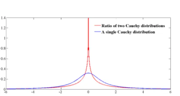
Unlike [9], where ZZ follows a Cauchy distribution, in our case, ZZ is ratio of two independent Cauchy distributions having the following density function ([20]) :
f(u) = logu
2
π2(u2−1) for − ∞< u <∞. (2)
Figure 1: Probability densities of Equation 1 and 2.
The function f(u) becomes infinite as u ap-proaches 0 and its value is indeterminate at
u=±1. But using l’Hˆopital’s rule it can be shown [20] thatf(u) approaches 1/π2asu ap-proaches±1. The density given in Equation 2 along with Equation 1 is plotted in Figure 1. Due to “not so nice property” of Equation 2, unlike [9], it is not straightforward to evalu-ate PrU(E). In the following, we discuss how this probability can be bounded from above.
3.2
Probability estimation
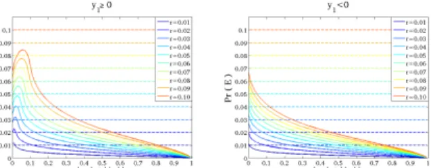
Letf(u) = π2log(u2u−21). First, consider the case wheny1>0. Suppose xy11 =r. Then,
PrU(E) = x1−y1 yR1 − y1 yR1 f(u)du= ry1−|y1| y1−|y1| − |y1| y1−|y1| f(u)du= r−k 1−k − k 1−k f(u)du (3) where, k = |y1y|
1 ∈ [0,1]. When y1 < 0, in a similar manner, it is easy to see that PrU(E) =
r+k 1−k k
1−k f(u)du. Note that the expression PrU(E) now is a function of two vari-ables r and k both of which take values in [0,1]. The combinations of r and k which are of interest are when, (a) r and k both are very close to zero. This corresponds to an in-terval of integration very close to origin where equation 2 differs significantly from equation 1, and, (b) when both r and k are close to 1, leading to an interval of integration which is larger than the symmetric half. To better understand the behavior PrU(E) as a function of
k and r, we do the following : (1) Fix any r ∈ [0,1], (2) Numerically evaluate the integral in equation 3 for different values of k ∈ [0,1] and fixed value of r as in step 1, (3) Repeat step 1 and 2 above, for various values of r. We show these plots in Figures 2, 3, 4, 5 respec-tively. In each of these figures, we plot PrU(E) vs k = |y1y|
1 for various values of r =
x1
Figure 2: Behavior of Pr(E) vs |y1|/y1 in the range
r ∈ [0.01,0.1] where the upper bound of Pr(E) is set to r
represented by the dashed lines.
Plot of PrU(E) for different values of r are shown using different col-ors. For each color (fixed r), the solid line represents the actual value of PrU(E) computed numerically for that fixed r and all k, while the dashed line of same color represents a con-stant value of PrU(E) for all k, which is set to be r in Figures 2, 3, and 0.8√r in Figures 4, 5 respectively.
Figure 3: Behavior of Pr(E) vs|y1|/y1 in the range r∈
[0.1,1.0] where the upper bound of Pr(E) is set torrepresented by the dashed lines.
One might guess that since we are merely using 1 norm in place of 2
norm and using similar analysis tech-nique as in [9], PrU(E) can be bounded from above by the quantity x1
2y1 = r
2, as was established in case of 2
norm [9]. It turns out that, that is not the case here. In fact, as can be seen from Figure 2, for small val-ues of rand k, the probability PrU(E)
is not bounded from above by any cr = cx1
y1 for c ≤ 1, which is understandable since according to Equation 3, this corresponds to integral of a small interval which is very close to the origin where equation 2 differs significantly from Equation 1 (Figure 1).
Figure 4: Behavior of Pr(E) vs |y1|/y1 in the range
r∈[0.01,0.1] where the upper bound of Pr(E) is set to 0.8√r
represented by the dashed lines.
Geometrically, this happens when,xis very close to the query point (which is origin in this case) while y is far away from the query point and the compo-nent of y along the direction xis very very small. Since both PrU(E) and r
take values in the interval [0,1], it is conceivable (from Figures 2 and 3) that PrU(E) may be bounded from above by a polynomial of r whose degree is
less than one (as we have seen, the bound doesn’t work1 for r and a potential bound could be of the form cra for any 0 < a < 1 and 0 < c < 1 since 0 ≤ r ≤ ra ≤ 1).
Figure 5: Behavior of Pr(E) vs |y1|/y1 in the range
r∈[0.1,1.0] where the upper bound of Pr(E) is set to 0.8√r represented by the dashed lines.
One might guess that the bound can take the form c√r for some c ∈ [0,1]. It turns out that, it is indeed the case and the value ofcis dictated by domain where r = 1 and k approaches 1, for
y1>0. Assumek= 1−for some small
positive , such that as → 0, k → 1. It is easy to see from Equation 3 that forr= 1 andk= 1−, the interval of the integral for Equation 3 is [−1+1,1].
For small values of, this interval of integration approaches (−∞,1] and due to symmetry of
1Note that, it may be possible to bound PrU(E) from above bycrfor somec>1. However, forr= 1 that is whenxandyare equidistant from the query point (measured using1norm), the bound becomes meaningless.
the density of ratio of two independent Cauchy random variables, the associated probability mass is clearly greater than 1/2, indicating that √r/2 can not be a valid upper bound either. It turns out, from Figures 4, 5 that 0.8√r works as a valid upper bound for all combinations ofk andr. For non zero query pointq, this insight leads to :
Proposition 3.1. Pick any q, x, y ∈ Rd with q−x1 ≤ q−y1. Pick a random direction
U ∈Rd whose coordinates are chosen uniformly at random from a Cauchy distribution. Then probability, over U, thatUy falls (strictly) betweenUq andUxis 54q−x1/q−y1.
3.3
Potential function and its effect on nearest neighbor search
For a queryq∈Rd and data pointsx1, x2, . . . , x
n∈Rd, letx(1), x(2), . . .denote a re-ordering of
the points by increasing1distance fromq. Define the potential function : ˜Φ(q,{x1, . . . , xn}) =
1
n
n
i=2
q−x(1)1/q−x(i)1. Note that ˜Φ∈[0,1] and this is very similar to the potential
function introduced in [9] i.e., Φ(q,{x1, . . . , xn}) = n1
n
i=2(q−x(1)2/q−x(i)2), except that
here, (a) 2 norm is replaced by 1 norm, and (b) linear function is replaced by a square root
function. Using ˜Φ, we analyze the failure probability of this new variant of RP tree next. Lemma 3.2. Pick any points q, x1, . . . , xn ∈ Rd. If these points are projected to a
direc-tion U ∈ Rd whose coordinates are chosen uniformly at random from a Cauchy
distribu-tion, then the expected fraction of the projected xi that fall between q and x(1) is at most
(4/5) ˜Φ(q,{x1, . . . , xn}).
Proof. LetZi be the event that x(i) falls betweenq andx(1) in the projection. Using
Propo-sition 3.1, PrU(Zi)≤ 45
q−x(1)1/q−x(i)1. The result now follows from linearity of
expectation.
Since the tree data structure partitions the input data space, any cell (at any level) of this tree contains only a subset of the n data pointsx1, . . . , xn. For any cell that contains m (m≤n) data points, the appropriate variant of the potential function is : ˜Φm(q,{x1, . . . , xn}) =
1 m m i=1 q−x(1)1/q−x(i)1.
Corollary 3.3. Pick any points q, x1, . . . , xn∈Rd and letS denotes any subset of thexi that
includes x(1). If q and the points in S are projected to a directionU ∈ Rd whose coordinates are chosen uniformly at random from a Cauchy distribution, then for any 0 < α < 1, the probability (overU) that at leastαfraction of the projectedS falls betweenqandx(1)is at most
(4/5) ˜Φ|S|(q,{x1, . . . , xn}).
Proof. Apply Lemma 3.2 toS noting that the corresponding value of ˜Φ is maximized whenS
consists of points closest toq measured using1 distance. The result now follows by applying
Markov’s inequality.
We are now ready to present the main result. In many of the statements below, we will drop the arguments (q,{x1, . . . , xn}) of ˜Φm(q,{x1, . . . , xn}) in the interest of readability. Theorem 3.4. Suppose a randomized partition tree is built using points {x1, . . . , xn} ⊂ Rd
according to Algorithm 1 and 2, and is used to answer a query q. Define β = 34 and l = log1/β(n/n0). Then over the randomizartion of tree construction, the probability that NN query does not return x(1) is at most 85li=0Φ˜βinln(5e/4 ˜Φβin).
Proof. Consider any internal node of the tree that contains qas well as mof the data points, including x(1). What is the probability that the split at that node separates q from x(1)? To
randomly-chosen split direction. Since the split point is chosen at random from an interval of mass 1/2, the probability that it separates q from x(1) is at most F/(1/2). Integrating out
F, we get : Prqis separated fromx(1)≤01Pr(F =f)1f/2df= 2
1 0Pr(F > f)df≤2 1 0 min 1,54f df= 204/5 ˜Φmdf+241/5 ˜Φ m 4 ˜Φm 5f df=85Φ˜mln 5e
4 ˜Φm , where, the second inequality uses Corollary 3.3. The result now follows by taking an union bound over the path that conveysqfrom root to leaf, in which the number of data points per level shrinks geometrically, by a factor of 3/4 or better.
The failure probability of nearest neighbor search using randomized partition trees as given in Theorem 3.4 is related to potential function ˜Φ which takes vales in the range [0,1]. The worst case happens when all points are equidistant from query point in 1 norm, in which
case ˜Φ is 1. However, under favorable condition, ˜Φmcan be bounded by a decreasing function of m. One such setting is when the query points are chosen arbitrarily but the data points used to construct the randomized tree data structure are drawn i.i.d. from an underlying distribution μ on Rd which is a doubling measure, i.e., there exists a constant C > 0 and a subset X ⊆ Rd such that μ(B(x,2r)) ≤ Cμ(B(x, r)) for allx ∈ X and allr > 0, where,
B(x, r) ={y ∈ Rd : x−y1 ≤r}. This essentially says that probability mass of an 1 ball
grows polynomially in its radius and an equivalent formulation is that, there exists a constant
d0 > 0 and a subset X ⊂ Rd such that for all x ∈ X, all r > 0 and al α ≥ 1, we have
μ(B(x, αr))≤αd0μ(B(x, r)). Comparing this with standard formula for the volume of a ball, the degree of polynomiald0= log2Ccan be thought ofdimension of measureμ. We next show
an upper bound for ˜Φmthat depends on only ond0and becomes useful especially whend0d.
Lemma 3.5. Supposeμ is continuous onRd and is a doubling measure of dimension d0≥2.
Pick anyq∈ X and drawx1, . . . , xn iid fromμ. Pick anyδ∈(0,1/2). With probability at least 1−3δover the choice of xi, for all2≤m≤n,Φ˜m(q,{x1, . . . , xn})≤6(
(2/m) ln(1/δ))1/d0 The proof is omitted due to space limitation. Using the above lemma, we conclude the following. Theorem 3.6. There is an absolute constant c0 for which the following holds. Suppose μ is a doubling measure on Rd of intrinsic dimension d0 ≥ 2. Pick any query q ∈ X and draw
x1, . . . , xn i.i.d. fromμ. With probability at least1−3δover the choice of data the tree fails to
return nearest neighbor is at mostc0(d0+ lnn0)((2/n0) ln(1/δ))1/d0 wheren0≥c09d0ln(1/δ).
The above theorem can be proved using Theorem 3.4 above and Lemma 12 from [9]. Note that, failure probability of Theorem 3.6 becomes an arbitrary small constant by choosingn0=
O(d0+ lnd0)2d0ln(1/δ). Moreover, for any small δ1 ∈ (0,1), the failure probability can be
made at most δ1, by constructing only O(log(1/δ1) independent randomized partition trees.
Note also that, the analysis presented here can be easily extended tok-nearest neighbor search fork≥1 which we do not discuss here due to space limitation.
4
Experimental evaluation
We evaluate empirical performance of our proposed algorithm on eight different real datasets2 of different dimensions as listed in Table 1. For each of these eight datasets, except
2The USPS dataset contains hand written digits. The AERIAL dataset contains texture information of large
areal photographs [19]. The COREL dataset is available at the UCI repository [2]. After removing the missing data and keep only 66,615 instances. MNIST is a dataset of handwritten digits. This SIFT and GIST dataset contains SIFT and GIST image descriptors, respectively, introduced in [14]. The original dataset contains 1 million image descriptors. We used 500000 image descriptors from this dataset for our experiments. The 20 NEWSGROUPS and REUTERS are common text datasets used in machine learning and are available in Matlab format in [6].
USPS, 20 NEWSGRUPS and REUTERS, we chose 50000 data points for our experiments. To generate a nearest neighbor search problem instance, we randomly selected 5000 data points as query points and used the remaining 45000 data points to construct data struc-tures for performing nearest neighbor search. After preprocessing, REUTERS, 20 NEWS-GROUPS ([6]) and USPS dataset contain less than 50000 data points each. In all these
Dataset No. of examples Dimensions
USPS 9298 256 AERIAL 275465 60 COREL 66615 89 MNIST 70000 784 SIFT 100000 128 GIST 50000 960 20 NEWSGROUPS 18846 26214 REUTERS 8293 18933
Table 1: Dataset description
cases, we randomly selected 5000 data points as query points and used the remaining data points to construct necessary data structures. Before presenting the actual results, we provide quanti-tative measurements that indicate the difficulty of nearest neighbor search for the eight datasets that we consider. Recall that the potential func-tion ˜Φ ∈ [0,1], and higher the value of ˜Φ, more
difficult the nearest neighbor search problem is, as this corresponds to the scenario where more and more data points are located in the vicinity of the true nearest neighbor of q. To estimate distribution of ˜Φ from data, we generated 20 nearest neighbor search prob-lem instances (each having 5000 random query points) as described above and computed
˜
Φ values for these 100,000 query instances. The histogram of these ˜Φ values are plotted in Figure 6. Quantitatively, Figure 6 suggests that three out of eight datasets, namely, GIST, 20 NEWSGROUPS and REUTERS are harder compared to the remaining five other datasets for answering nearest neighbor queries and we will see later that experimental evaluations agree with this observation.
Figure 6: Histogram of potential function ˜Φ for differ-ent datasets.
For our comparison, we used the LSH scheme proposed in [11] for 1 norm in
non-Hamming space. We used the random hash function,hU,b(x) =U
x+b
w that a maps vec-tor x∈Rd to an integer, whereU ∈Rd is a random vector whose entries are chosen i.i.d. from a 1-stable (Cauchy) distribution, w is the width of projection, and b is a real
num-ber chosen uniformly from the range [0, w]. We tried different values for the number of projec-tionsk, namelyk= 2,4,8,16,32,64 and 128 and report the results for k= 32 andk= 64 due to space limitations. It was observed that small values of k resulted in very large number of retrieved points as compared to RP tree, thus, essentially doing a linear search while large val-ues ofkresulted in small number of retrieved points however, yielding a poor nearest neighbor search accuracy. The results for eight different datasets are presented in Figure 7, where each panel plots number of retrieved data points vs 1-NN accuracy. These results are based on 20 random instances of nearest neighbor search problems, where in every problem instance, 5000 data points were chosen at random as query points and the rest were used to build the data structures (RP trees / hash tables). The 1-NN accuracy of nearest neighbor search was simply calculated as fraction of the query points for which the true nearest neighbor was within the retrieved set of points returned by respective methods (RP trees or LSH). In each of the plots in Figure 7, the markers (legends) represent number of trees / hash tables (N) used. We used seven different values forN, namely, 2, 4, 8, 16, 32, 64 and 128. The placement of marker and the associatedN values are easy to identify since accuracy increases withN.
As can be seen from Figure 7, except for GIST, 20 NEWSGROUPS and REUTERS datasets, the proposed RP tree method clearly achieves better 1-NN accuracy with fewer retrieved data points as compared to LSH. Note that LSH as well as the proposed method do not work well
Figure 7: 1-NN accuracy vs number of retrieved data points.
for the GIST dataset. This can be attributed to the fact that majority of the query points have very high potential function values for the GIST dataset (Figure 6), indicating that performing nearest neighbor search on GIST dataset is a difficult problem. Performance of the proposed method is marginally better than that of LSH for the 20 NEWSGROUPS and REUTERS datasets, without clear distinct advantage over LSH. Moreover, in order to achieve close to 100% 1-NN accuracy for these two datasets, both the methods essentially scans the whole dataset. This phenomenon can most likely be explained due to the facts that : (a) for both datasets, majority of the query points have very high potential function values, and (b) these two datasets have very high dimensions compared to the other datasets and the number of data points used to construct the data structures is much less as compared to the other datasets.
Note that fiixing the parameters of LSH scheme, namelyw, k, N, doesn’t give an estimate of the number of retrieved data points and can vary quite widely based on the choice ofwand
k. RP trees on the other hand, give an easy-to-understand upper bound on the number of retrieved points, namelyn0N, where,N is the number of trees andn0is maximum number of
points in any leaf node. In addition, time complexity of nearest neighbor search depends on two factors, (a) time spent in reaching leaf node/hash bucket (number dot product computation required), and (b) time spent in distance computation for all points within the retrieved set. Under restricted setting, traditional analysis of LSH ([12, 1]) sets number of projectionkto be
O(logn). By construction, depth of our randomized partition tree is alsoO(logn). Assuming that tree/hash table data structures are constructed off-line, time required for a query point to reach the appropriate leaf node/hash bucket takes time of the same order. Because of smaller number of retrieved points, RP based method works faster with better accuracy. It was observed that changing differentw, k, N combination can reduce the number of retrieved points in LSH and hence query time, at the expense of worse 1-NN accuracy.
5
Conclusion
In this paper, we have presented a new variant of randomized partition tree that can efficiently answer nearest neighbors queries in high dimensions when distances are measured using using
1 norm. We have presented analysis of its failure probability in finding true nearest neighbor
and have shown that failure probability can be arbitrarily small constant when data are drawn i.i.d from a doubling measure and the query point is arbitrary. Our experimental evaluations suggest that the proposed method achieves better accuracy with fewer retrieved data points as compared to LSH using 1-stable distribution for 1norm nearest neighbor search.
References
[1] A. Andoni and P. Indyk. Near-Optimal Hashing Algorithms for Approximate Nearest Neighbor in High Dimensions. Communications of the ACM, 51(1):117–122, 2008.
[2] K. Bache and M. Lichman. UCI machine learning repository, 2013. Available at : http:// archive.ics.uci.edu/ml.
[3] A. Beygelzimer, S. Kakade, and J. Langford. Cover Trees for Nearest Neighbor. In23rd Interna-tional Conference on Machine Learning, 2006.
[4] B. Brinkman and M. Charikar. On the Impossibility of Dimension Reduction in1. In44th Annual Symposium on Foundations of Computer Science, 2003.
[5] B. Brinkman and M. Charikar. On the Impossibility of Dimension Reduction in1.Journal of the ACM, 52(2):766–788, 2005.
[6] D. Cai. Text Dat sets in Matlab Format, 2009. Available at : http://www.cad.zju.edu.cn/home/ dengcai/Data/TextData.html.
[7] J. M. Chambers, C. L. Mallows, and B. W. Stuck. A Method for Simulating Stable Random Variables. Journal American Statistical Association, 71:340–3443, 1976.
[8] S. Dasgupta and A. Gupta. An Elementary Proof of a Theorem of Johnson-Lindenstrauss.Random Structures and Algorithms, 22(1):60–65, 2003.
[9] S. Dasgupta and K. Sinha. Randomized Partition Trees for Exact Nearest Neighbor Search. In The 26th Annual Conference on Learning Theory, 2013.
[10] S. Dasgupta and K. Sinha. Randomized Partition Trees for Nearest Neighbor Search.Algorithmica, 72(1):237–263, 2015.
[11] M. Datar, N. Immorlica, P. Indyk, and C. S. Mirrokni. Locality-Sensitive Hashing Based on p-Stable Dis. InThe 20th ACM Symposium on Computational Geometry, 2004.
[12] A. Gionis, P. Indyk, and R. Motwan. Similarity search in high dimensions via hashing. In25th International Conference on Very Large Databases, 1999.
[13] P. Indyk. Stable Distributions, Pseudorandom Generators, Embeddings, and Data Stream Com-putation. Journal of the ACM, 53(3):307–323, 2006.
[14] H. J´egou, M. Douze, and C. Schmid. Product quantization for nearest neighbor search. IEEE Transactions on Pattern Analysis and Machine Intelligence, 33(1):117–128, 2011.
[15] W. B. Johnson and J. Lindenstrauss. Extensions of Lipschitz Mapping into Hilbert Space. Con-temporary Mathematics, 26:189 – 206, 1984.
[16] D. R. Karger and M. Ruhl. Finding Nearest Neighbors in Growth Restricted Metrics. In 34th Annual ACM Symposium on Theory of Computing, 2002.
[17] R. Krauthgamer and J. Leel. Navigating Nets : Simple Algorithms for Proximity Search. In15th Annual Symposium on Discrete Algorithms, 2004.
[18] J. R. Lee and A. Naor. Embedding the Diamond Graph in p and Dimension Reduction in 1. Geometric and Functional Analysis, 14(4):745–747, 2004.
[19] B. S. Manjunath and W. Y. Ma. Texture features for browsing and retrieving of large image data. IEEE Transactions on Pattern Analysis and Machine Intelligence, 33(1):117–128, 2011.
[20] P. R. Rider. Distributions of Product and Quotient of Cauchy Variables. The American mathe-matical Monthly, 72(3), 1965.
[21] K. Sinha. LSH vs Randomized Partition Trees : Which One to Use for Nearest Neighbor Search? In13th International Conference on Machine Learning and Applications, 2014.