An efficient approach of face detection and recognition from digital images for modern security and office hour attendance system

An Efficient Approach of Face Detection

and Recognition from Digital Images for

Modern Security and Office Hour

Attendance System

by

Md. Kamrul Islam. Anik

Submitted to the Department of Computer Science and Engineering

In partial fulfillment of the requirements for the degree of Bachelor of Science December 2015

i

CONTACT INFORMATION

Author:

Md. Kamrul Islam. Anik

ID: 11301014

e-mail:

[email protected]

Supervisor:

Samiul Islam

e-mail:

[email protected]

Co-supervisor:

Khadija Rasul

e-mail:

[email protected]

Department Of Computer Science And Engineering Internet: www.bracu.ac.bd

BRAC University Phone: +880-2-9844051-4, Ext-4003

66 Mohakhali +880-2-9853948-9

Dhaka – 1212 Fax: +880-2-58810383,

ii

ABSTRACT

The purpose of this project is to make an efficient security system for university safety measurement which can also be used to calculate the office hours of Student Tutors by face detection and recognition. By using surveillance cameras, attached at all the entrance of university main buildings, the system can detect human faces and then it can recognize people. First, the system captures the image of a person who enters into the building and then detects the face from the image. Then the recognition system matches that image with the given database of images with valid information. After matching that image if the system recognize that face it gives a green signal to allow that person. Otherwise, if the system cannot recognize that face it gives an alert signal to block that person as an intruder. Also, this system calculates the office hours of the Student Tutors. By using face recognition the system takes the starting time and ending time of the Student Tutors individually and then gives the result as output by calculating the time duration.

iii

ACKNOWLEDGEMENT

Before starting to write this paper, I would like to express my gratitude to Almighty Allah (SWT) who gave me the opportunity, determination, strength and intelligence to complete my thesis. I want to acknowledge my fellow classmates who have consistently support me

throughout the thesis. I would like to thank my supervisor Samiul Islam and my co-supervisor

Khadija Rasul sincerely for their consistent supervision, guidance and unflinching encouragement in accomplishing my work and help me to present my idea properly.

iv

CONTENTS

Chapter 2- Background Study 04

2.1 Digital Image ……….….. 04 2.2 Pixel ……….…… 04 2.3 Raster Images ………..…. 05 2.4 RGB Color Model ………...…. 05 2.5 Grayscale ………..……… 06 2.6 RGB to Grayscale ………...……. 06 2.7 Image Processing ………. 06 2.8 Face Detection ………..………… 07 2.9 Face Recognition ……….………. 07 2.10 Biometrics ……….. 07 2.11 Biometric Verification ………...……… 07 Related Work 08

Chapter 3- Face Detection 09

3.1 Integral Image ……….……. 09

3.2 Cascade ……… 10

3.3 Haar Cascade Classifiers ……….…. 10

3.4 Haar Features ……….…….. 11 3.5 AdaBoost ……….………. 11 3.6 Feature Detection ……….……… 12 3.7 Object Detection ……….. 12 3.8 Viola-Jones Algorithm ………. 13 3.8.1 Properties ………... 14 3.8.2 Methods ……….……. 14

3.9 Face Detection Results ………...….. 15

Chapter 4- Face Recognition 16

4.1 Principal Component Analysis (PCA) ………...….. 16

4.2 Eigenfaces ……… 17

4.3 Eigen Values and Eigen Vectors ………..… 18

4.4 Calculations of Eigen Values and Eigen Vectors ………...……. 18

4.5 Repeated Eigenvalues ……….…. 18

4.6 Face Image Normalization ………..………. 19

4.6.1 Face Image Scaling ……….… 19

4.6.2 Conversion to Grayimage ……….….. 20

4.7 Database of Face Images ………. 20

4.8 Face Recognition Methodology ……….………….. 22

4.9 Training Set of Images ……….……… 23

v

Page

Chapter 5- Application 26

5.1 Implementation ………...…. 26

5.2 Result Analysis ………..….. 28

5.3 Face Detection and Recognition Results ………...….. 30

Chapter 6- Future Work Plan 32

Conclusion 32

References 33

LIST OF FIGURES

Figure 2: Pixel ………...……… 04

Figure 3: RGB Color Model ………..……….…. 05

Figure 4: Grayscale ………..……… 05

Figure 5: Integral image generation ……….…….. 09

Figure 6: Cascade of stages ………. 10

Figure 7: Common Haar-like features ……….……….. 10

Figure 8: Examples of Haar features ………. 11

Figure 9: Input Images (a,b,c) ………. 15

Figure 10: Detected Faces from the images (a,b,c) ……….……….. 15

Figure 11: Detected Face Images (a,b,c) ………..…….. 19

Figure 12: Resized & Cropped Images (a,b,c) ………...………… 19

Figure 13: RGB Image ………. 20

Figure 14: Grayimage ……….………. 20

Figure 15: Red Image ……….. 20

vi

Figure 17: Blue Image ………..…… 20

Figure 18: Sample Train Database ………. 21

Figure 19: Sample Test Database ………..……. 22

Figure 20: Sample Result 1 (a,b,c) ……….………. 30

Figure 21: Sample Result 2 (a,b,c) ………..……… 30

Figure 22: Sample Result 3 (a,b,c) ………..… 30

Figure 23: Sample Result 4 (a,b,c) [Twins 1] ……….………… 31

Figure 24: Sample Result 5 (a,b,c) [Twins 2] ………...….. 31

Figure 25: Sample Result 6 (a,b,c) ………..… 31

LIST OF TABLES

Table 2: Face Detection Procedure ………. 28

Table 3: Face Recognition Procedure ……… 28

1

Chapter 1

INTRODUCTION

To enter in a restricted or reserved area people are still using a human guard to check the ID cards which is not absolutely safe or efficient in this modern age. Moreover this system is easy to break through, as any person can use others ID cards or make a duplicate one. As each & every human faces are unique, so for recognizing the correct people it‟s much convenient if a machine can detect a human face and recognize it for the entrance, which will be efficient and absolutely work without any man power. Punch cards and finger prints are using now a day by some offices and universities for a secure entrance, though this is detected by a machine but still there are some safety issue. The card can be stolen or the card holders can lose it.

There are two parts in our project to make this a real time workable program. First one is detecting faces from an input image, which can be captured by surveillance cameras or webcams. The second part is recognizing that detected face with other face images which is already in the database. We have done the first part by Viola-Jones face or object detecting algorithm [4]. For the second part of recognition we used PCA (Principal Component Analysis) based face recognition system [7][13][14].

The ability of human to recognize faces is remarkable though, it is very difficult for a machine to recognize different faces individually. Human can recognize thousands of faces learned throughout their life time and identify familiar faces at a glance even after years of separation. This skill is quite robust, despite large changes in the visual stimulus due to viewing conditions, expression, aging and distractions such as glasses, beards or changes in hair style. Developing a computational model of face recognition is quite difficult, because faces are complex, multi-dimensional visual stimuli. They are a natural class of objects and stand in stark contrast to sine wave gratings, the “blocks world” and other artificial stimuli used in human and computer vision research. Thus unlike most early visual functions, for which we may construct detailed models of retinal or striate activity, face recognition is a very high level task for which computational approaches can currently only suggest broad constraints on the corresponding neural activity. We therefore focused our research towards developing a sort of early, preattentive pattern [13] recognition capability that does not depend upon having full three-dimensional models or detailed geometry. Our aim was to develop a computational model of face recognition which is fast, reasonably simple and accurate in constrained environments such as office, household or an educational institute.

Although face recognition is a high level visual problem, there is quite a bit of structure imposed on the task. We take advantages of some of this structure by proposing a scheme for recognition

2

which is based on an information theory approach, seeking to encode the most relevant information in a group of faces which will best distinguish them from one another. The approach transforms face images into a small set of characteristic feature images, called “Eigenfaces”, which are the principal components of the initial training set of face images. Recognition is performed by projecting a new image into the sub space spanned by the eigenfaces (“face space”) and then classifying the face by comparing its position in face space with the positions of known individuals. Automatically learning and later recognition is practical within this framework. Recognition under reasonable varying conditions is achieved by training on a limited number of characteristic views (e.g. a “straight on” view, a 45° view and a profile view). The approach has advantages over other face recognition schemes in its speed and simplicity, learning capacity and relative insensitivity to small or gradual changes in the face image [13].

1.1 Objectives:

The goal of this project is to make an automated security system for the university which is much more authentic and can be worked without any man power. Also we are trying to provide an efficient office hour calculating system which is much better and reliable than card punch or thumb scanner hour calculating system. This system also uses Artificial Intelligence (AI) to learn from its input and remember those features for future face detection and recognition.

1.2 Scopes:

Face detection and recognition system is a very modern technology which is a combination of Image Processing and Artificial Intelligence. If a system can be run based on this technology it can be much more helpful for other aspects of modern technology like robotics, medical science, bio-technology, banking system, scientific research work and many others.

1.3 Limitations:

It is very difficult for a machine to recognize different faces individually and remember them. Without matching the skin colors or knowing whether it‟s a male or a female face, recognizing a face is a very difficult process for a machine. The machine can recognize human faces by comparing only several features of the human face and this is very challenging to find out the same person whether s/he has a different facial expression, whether they are wearing glasses or have beards. Also some are identical twins, which is another challenge to identify both of them separately. Another most challenging and significant part of this project is to make a database of human faces and then train the system with the huge number of face image dataset.

3

1.4 Research Questions:

Q.01: How can a machine detect a human face from an image? Q.02: Can the system detect multiple faces in the same image? Q.03: How the Viola-Jones algorithm can detect human faces? Q.04: How can a machine recognize a human face?

Q.05: What is Principal Component Analysis? Q.06: What are Eigen Faces and Eigen Vectors?

4

Chapter 2

BACKGROUND STUDY

2.1 Digital Image:

A digital image is a numeric representation (normally binary) of a two-dimensional image. Depending on whether the image resolution is fixed, it may be of vector or raster type. By itself, the term "digital image" usually refers to raster images or bitmapped images. Digital image is a two dimensional array of pixels. Each pixel has an intensity value which is represented by a digital number and a location address which is referenced by its row and column numbers.

Figure 1: Digital Image (2D) Figure 2: Pixel

2.2 Pixel:

In digital imaging, a pixel or picture element is a physical point in a raster image, or the smallest addressable element in an all points addressable display device; so it is the smallest controllable element of a picture represented on the screen. One color is representing a tiny little area of the picture. A digital color image pixel is just numbers representing a RGB data value (Red, Green, Blue). Each pixel‟s color sample has three numerical RGB components (Red, Green, Blue) to represent the color of that tiny pixel area. These three RGB components are three 8-bit numbers for each pixel. Three 8-bit bytes (one byte for each of RGB) are called 24 bit color. Each 8-bit

5

RGB component can have 256 possible values, ranging from 0 to 255. For example, three values like (250, 165, 0), meaning (Red=250, Green=165, Blue=0) to denote one Orange pixel.

2.3 Raster Images:

Raster images have a finite set of digital values, called picture elements or pixels. The digital image contains a fixed number of rows and columns of pixels. Pixels are the smallest individual element in an image, holding quantized values that represent the brightness of a given color at any specific point. Typically, the pixels are stored in computer memory as a raster image or raster map, a two-dimensional array of small integers. These values are often transmitted or stored in a compressed form.

2.4 RGB Color Model:

The RGB color model is an additive color model in which red, green, and blue light are added together in various ways to reproduce a broad array of colors. The name of the model comes from the initials of the three additive primary colors, red, green, and blue. The main purpose of the RGB color model is for the sensing, representation, and display of images in electronic systems, such as televisions and computers, though it has also been used in conventional photography.

6

2.5 Greyscale:

In photography and computing, a grayscale digital image is an image in which the value of each pixel is a single sample, that is, it carries only intensity information. Images of this sort, also known as black-and-white, are composed exclusively of shades of gray, varying from black at the weakest intensity to white at the strongest. Grayscale images are distinct from one-bit bi-tonal black-and-white images, which in the context of computer imaging are images with only the two colors, black, and white (also called bilevel or binary images). Grayscale images have many shades of gray in between. Often, the grayscale intensity is stored as an 8-bit integer giving 256 possible different shades of gray from black to white. If the levels are evenly spaced then the difference between successive graylevels is significantly better than the graylevel resolving power of the human eye. Grayscale images are very common, in part because much of today's display and image capture hardware can only support 8-bit images. In addition, grayscale images are entirely sufficient for many tasks and so there is no need to use more complicated and harder-to-process color images.

2.6 RGB to Grayscale:

There are 3 ways to convert a color or RGB image to a Grayscale or black and white image - (i) Lightness Method: The lightness method averages the most prominent and least prominent colors: (max(R, G, B) + min(R, G, B)) / 2.

(ii) Average Method: The average method simply averages the values: (R + G + B) / 3.

(iii) Luminosity Method: The luminosity method is a more sophisticated version of the average method: 0.21 R + 0.72 G + 0.07 B.

2.7 Image Processing:

Image processing is a method to convert an image into digital form and perform some operations on it, in order to get an enhanced image or to extract some useful information from it. It is a type of signal dispensation in which input is image, like video frame or photograph and output may be image or characteristics associated with that image. Usually Image Processing system includes treating images as two dimensional signals while applying already set signal processing methods to them.

7

2.8 Face Detection:

In digital camera terminology face detection, also called face-priority AF (auto focus), is a function of the camera that detects human faces so that the camera can set the focus and appropriate exposure for the shot automatically. When using a flash, face detection will also usually and automatically correct or remove the unwanted red-eye effect that can often occur when photographing people using a flash.

2.9 Face Recognition:

Facial recognition (or face recognition) is a type of biometric software application that can identify a specific individual in a digital image by analyzing and comparing patterns. Facial recognition systems are commonly used for security purposes but are increasingly being used in a variety of other applications. This is a type of biometrics that uses images of a person's face for recognition and identification.

2.10 Biometrics:

Biometrics is the measurement and statistical analysis of people's physical and behavioral characteristics. The technology is mainly used for identification and access control, or for identifying individuals that are under surveillance. The basic premise of biometric authentication is that everyone is unique and an individual can be identified by his or her intrinsic physical or behavioral traits. (The term "biometrics" is derived from the Greek words "bio" meaning life and "metric" meaning to measure.)

2.11 Biometric Verification:

Biometric verification is any means by which a person can be uniquely identified by evaluating one or more distinguishing biological traits. Unique identifiers include fingerprints, hand geometry, earlobe geometry, retina and iris patterns, voice waves, DNA, and signatures. The oldest form of biometric verification is fingerprinting. Historians have found examples of thumbprints being used as a means of unique identification on clay seals in ancient China. Biometric verification has advanced considerably with the advent of computerized databases and the digitization of analog data, allowing for almost instantaneous personal identification.

8

RELATED WORK

Much of the work in computer recognition of faces has focused on detecting individual features such as the eyes, nose, mouth, head outline and defining a face model by the position, size and relationships among these features. Beginning with Bledsoe‟s and Kanade‟s early systems, a number of automated or semi-automated face recognition strategies have modeled and classified faces based on normalized distances and ratios among feature points. Recently this general approach has been continued and improved by the recent work of Yuille et al. Such approaches have proven difficult to extend to multiple views and have often been quite fragile. Research in human strategies of face recognition, moreover, has shown that individual features and their immediate relationships comprise an insufficient representation to account for the performance of adult human face identification. Nonetheless, this approach to face recognition remains the most popular one in the computer vision literature [13][14].

Connectionist approaches to face identification seek to capture the configurational or gestalt-like nature of the task. Fleming and Cottrell building on earlier work by Kohonen and Lahtio, use nonlinear units to train a network via back propagation to classify face images. Stonham‟s WISARD system has been applied with some success to binary face images, recognizing both identity and expression. Most connectionist systems dealing with faces treat the input image as a general 2-D pattern and can make no explicit use of the configurational properties of a face. Only very simple systems have been explored to date and it is unclear how they will scale to larger problems.

Recent work by Burt et al. uses a “smart sensing” approach based on multiresolution template matching. This coarse-to-fine strategy uses a special purpose computer built to calculate multiresolution pyramid images quickly and has been demonstrated identifying people in near-real-time. The face models are built by hand from face images [13][14].

9

Chapter 3

FACE DETECTION

Face detection proposed by Viola and Jones is most popular among the face detection approaches based on statistics methods. This face detection is a variant of the AdaBoost algorithm which achieves rapid and robust face detection. They proposed a face detection framework based on the AdaBoost learning algorithm using Haar features. This can be applied on real time face detection. The face detection algorithm looks for specific Haar features of a human face. When one of these features is found, the algorithm allows the face candidate to pass to the next stage of detection. A face candidate is a rectangular section of the original image called a sub-window. Generally these sub-windows have a fixed size (typically 24×24 pixels). This sub-window is often scaled in order to obtain a variety of different size faces. The algorithm scans the entire image with this window and denotes each respective section a face candidate [3].

3.1 Integral Image:

The simple rectangular features of an image are calculated using an intermediate representation of an image, called the integral image. The integral image is an array containing the sums of the pixels‟ intensity values located directly to the left of a pixel and directly above the pixel at location (x,y) inclusive. So if A[x,y] is the original image and AI[x,y] is the integral image then the integral image is computed as AI [ x , y ] = ∑ A( x', y' ) [1][3].

Figure 5: Integral image generation. The shaded region represents the sum of the pixels up to position (x,y) of the image. It shows a 3x3 image and its integral image representation.

10

3.2 Cascade:

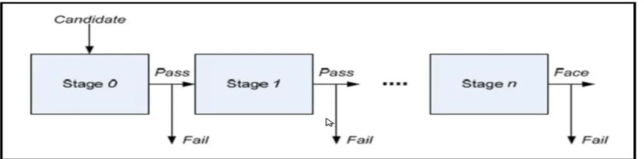
The Viola and Jones face detection algorithm eliminates face candidates quickly using a cascade of stages. The cascade eliminates candidates by making stricter requirements in each stage with later stages being much more difficult for a candidate to pass. Candidates exit the cascade if they pass all stages or fail any stage. A face is detected if a candidate passes all stages [3].

Figure 6: Cascade of stages. Candidate must pass all stages in the cascade to be concluded as a face.

3.3 Haar Cascade Classifiers:

The core basis for Haar classifier object detection is the Haar-like features. These features, rather than using the intensity values of a pixel, use the change in contrast values between adjacent rectangular groups of pixels. The contrast variances between the pixel groups are used to determine relative light and dark areas. Two or three adjacent groups with a relative contrast variance form a Haar-like feature [1][5].

11

3.4 Haar Features:

Haar features are composed of either two or three rectangles. Face candidates are scanned and searched for Haar features of the current stage. The weight and size of each feature and the features themselves are generated using a machine learning algorithm from AdaBoost [3].

Figure 8: Examples of Haar features. Areas of white and black regions are multiplied by their respective weights and then summed in order to get the Haar feature value.

3.5 AdaBoost:

AdaBoost, short for "Adaptive Boosting", is a machine learning meta-algorithm formulated by Yoav Freund and Robert Schapire. It can be used in conjunction with many other types of learning algorithms to improve their performance. The output of the other learning algorithms ('weak learners') is combined into a weighted sum that represents the final output of the boosted classifier. AdaBoost is adaptive in the sense that subsequent weak learners are tweaked in favor of those instances misclassified by previous classifiers. AdaBoost is sensitive to noisy data and outliers. In some problems, however, it can be less susceptible to the overfitting problem than other learning algorithms. The individual learners can be weak, but as long as the performance of each one is slightly better than random guessing (e.g., their error rate is smaller than 0.5 for binary classification), the final model can be proven to converge to a strong learner, While every learning algorithm will tend to suit some problem types better than others, and will typically have many different parameters and configurations to be adjusted before achieving optimal performance on a dataset, AdaBoost (with decision trees as the weak learners) is often referred to as the best out-of-the-box classifier. When used with decision tree learning, information gathered at each stage of the AdaBoost algorithm about the relative 'hardness' of each training sample is fed into the tree growing algorithm such that later trees tend to focus on harder-to-classify examples.

AdaBoost refers to a particular method of training a boosted classifier. A boost classifier is a classifier in the form

12

where each is a weak learner that takes an object as input and returns a real valued result indicating the class of the object. The sign of the weak learner output identifies the predicted object class and the absolute value gives the confidence in that classification. Similarly, the -layer classifier will be positive if the sample is believed to be in the positive class and negative otherwise.

Each weak learner produces an output, hypothesis , for each sample in the training set. At

each iteration , a weak learner is selected and assigned a coefficient such that the sum training error of the resulting -stage boost classifier is minimized.

Here is the boosted classifier that has been built up to the previous stage of

training, is some error function and is the weak learner that is being

considered for addition to the final classifier.

3.6 Feature Detection:

In computer vision and image processing the concept of feature detection refers to methods that aim at computing abstractions of image information and making local decisions at every image point whether there is an image feature of a given type at that point or not. The resulting features will be subsets of the image domain, often in the form of isolated points, continuous curves or connected regions.

3.7 Object Detection:

Object detection is the process of finding instances of real-world objects such as faces, bicycles, and buildings in images or videos. Object detection algorithms typically use extracted features and learning algorithms to recognize instances of an object category. Object recognition is a task of finding and identifying objects in an image or video sequence. Humans recognize a multitude of objects in images with little effort, despite the fact that the image of the objects may vary somewhat in different viewpoints, in many different sizes and scales or even when they are translated or rotated. Objects can even be recognized when they are partially obstructed from

13

view. This task is still a challenge for computer vision systems. Many approaches to the task have been implemented over multiple decades.

3.8 Viola-Jones Algorithm:

The Cascade Object Detector uses the Viola-Jones algorithm to detect people's faces, noses, eyes, mouth, or upper body.

detector = vision.CascadeObjectDetector creates a System object „detector‟, that detects objects using the Viola-Jones algorithm. The ClassificationModel property controls the type of object to detect. By default, the Detector is configured to detect faces.

detector = vision.CascadeObjectDetector(MODEL) creates a System object, detector, configured to detect objects defined by the input string, MODEL. The MODEL input describes the type of object to detect. There are several valid MODEL strings, such as 'FrontalFaceCART', 'UpperBody', and 'ProfileFace'.

The ClassificationModel is - Trained cascade classification model. Train cascade classification model, specified as a comma-separated pair consisting of „ClassificationModel‟ and a string. This value sets the classification model for the detector. It can be trained a custom classification model using the trainCascadeObjectDetector function. The function can train the model using Haar-like features, histograms of oriented gradients (HOG), or local binary patterns (LBP). The CassificationModel is set as Default: FrontalFaceCARTmodel string.

detector = vision.CascadeObjectDetector(XMLFILE) creates a System object,detector, and configures it to use the custom classification model specified with theXMLFILE input. The XMLFILE can be created using the trainCascadeObjectDetectorfunction or OpenCV (Open Source Computer Vision) training functionality. We have to specify a full or relative path to the XMLFILE.

detector = vision.CascadeObjectDetector(Name,Value) configures the cascade object detector object properties. You specify these properties as one or more name-value pair arguments. Unspecified properties have default values.

BBOX = step(detector,I) returns BBOX, an M-by-4 matrix defining M bounding boxes containing the detected objects. This method performs multi scale object detection on the input image, I. Each row of the output matrix, BBOX, contains a four-element vector, [x y width height], that specifies in pixels, the upper left corner and size of a bounding box. The input image I must be a gray scale or true color (RGB) image.

14

BBOX = step (Detector, I, roi) detects objects within the rectangular search region specified by roi. It is a must to specify roi as a 4-element vector, [xywidthheight], that defines a rectangular region of interest within image I& set the 'UseROI' property to true to use this syntax. UseROIis – Use region of interest. [false (default) | true]

Use region of interest, specified as a comma-separated pair consisting of „UseROI‟ and a logical scalar. Set this property to true to detect objects within a rectangular region of interest within the input image.

3.8.1 Properties:

 ClassificationModel – Trained cascade classification model

 MinSize – Size of smallest detectable object

 MaxSize – Size of largest detectable object

 ScaleFactor – Scaling for multi scale object detection

 MergeThreshold – Detection threshold

 UseROI – Use region of interest [false (default) | true]

3.8.2 Methods:

 clone - Create cascade object detector object with same property values

 getNumInputs - Number of expected inputs to step method

 getNumOutputs - Number of outputs from step method

 isLocked - Locked status for input attributes and non-tunable properties

 release - Allow property value and input characteristics changes

15

3.9 Face Detection Results:

a. a.

b. b.

c. c.

Figure 9: Input Images Figure 10: Detected Faces from the images.

16

Chapter 4

FACE RECOGNITION

4.1 Principal Component Analysis (PCA):

Principal component analysis (PCA) is a statistical procedure that uses an orthogonal transformation to convert a set of observations of possibly correlated variables into a set of values of linearly uncorrelated variables called principal components. The number of principal components is less than or equal to the number of original variables. This transformation is defined in such a way that the first principal component has the largest possible variance (that is, accounts for as much of the variability in the data as possible), and each succeeding component in turn has the highest variance possible under the constraint that it is orthogonal to the preceding components. The resulting vectors are an uncorrelated orthogonal basis set. The principal components are orthogonal because they are the eigenvectors of the covariance matrix, which is symmetric. PCA is sensitive to the relative scaling of the original variables [16].

PCA is one of the most successful techniques that have been used in face recognition. The objective of the Principal Component Analysis is to take the total variation on the training set of faces and to represent this variation with just some little variables. When we are working with great amounts of images, reduction of space dimension is very important. PCA intends to reduce the dimension of a group or to space it better so that the new base describes the typical model of the group. The maximum number of principal components is the number of variables in the original space. Even so to reduce the dimension, some principal components should be omitted [7]. In the PCA approach the component matching relies on good data to build eigenfaces. In other words, it builds M eigenvectors for an N x M matrix. They are ordered from largest to lowest where the largest eigenvalue if associated with the vector that finds the most variance in the image. To classify an image the eigenface with smallest Euclidean distance from the input face has been find out. For this purpose input image has been transformed to a lower dimension M’ by computing,

[v1 v2 … vM]^T

Where each vi = wi * ei ^T, viis the ith coordinate of the facial image in the new space, which came to be the principal component. The vectors ei, also called eigenimages, can also be represented as images and look like faces. These vectors represent the classes of faces to which a new instance of a face has been classified. Now with the help the transformed M the vector k has been find out to which the image is the closest [15].

17

Omega(Ω) represent the contribution of each eigenface to the representation of an image in a basis constructed from the eigenvectors. Then k has been find out such that

εk = || Ω - Ω k|| < Θ

Where Ω k is the vector describing the kth face class. When εk is less than some threshold value Θ the new face is classified to belong to class k [15].

4.2 Eigenfaces:

Eigenfaces refers to an appearance-based approach to face recognition that seeks to capture the variation in a collection of face images and use this information to encode and compare images of individual faces in a holistic (as opposed to a parts-based or feature-based) manner. Specifically, the eigenfaces are the principal components of a distribution of faces, or equivalently, the eigenvectors of the covariance matrix of the set of face images, where an image with N pixels is considered a point (or vector) in N-dimensional space. The idea of using principal components to represent human faces was developed by Sirovich and Kirby (Sirovich and Kirby 1987) and used by Turk and Pentland (Turk and Pentland 1991) for face detection and recognition. The Eigenface approach is considered by many to be the first working facial recognition technology, and it served as the basis for one of the top commercial face recognition technology products. Since its initial development and publication, there have been many extensions to the original method and many new developments in automatic face recognition systems. Eigenfaces is still often considered as a baseline comparison method to demonstrate the minimum expected performance of such a system [9][13][14].

The motivation of Eigenfaces is twofold:

 Extract the relevant facial information, which may or may not be directly related to human intuition of face features such as the eyes, nose, and lips. One way to do so is to capture the statistical variation between face images.

 Represent face images efficiently. To reduce the computation and space complexity, each face image can be represented using a small number of parameters.

The eigenfaces may be considered as a set of features which characterize the global variation among face images. Then each face image is approximated using a subset of the eigenfaces, those associated with the largest eigenvalues. These features account for the most variance in the training set [9][13]14].

18

4.3 Eigen Values and Eigen Vectors:

In linear algebra, the eigenvectors of a linear operator are non-zero vectors which, when operated on by the operator, result in a scalar multiple of them. The scalar is then called the eigenvalue (λ) associated with the eigenvector(X). Eigen vector is a vector that is scaled by a linear transformation. It is a property of a matrix. When a matrix acts on it, only the vector magnitude is changed not the direction.

AX = λX ………. (1) Where A is a Vector function [15].

4.4 Calculations of Eigen Values and Eigen Vectors:

(A-λI)X = 0 ………. (2)

Where I is the n x n Identity matrix. This is a homogeneous system of equations, and from fundamental linear algebra, it has been proved that a nontrivial solution exists if and only if

D(A-λI) = 0 ………. (3)

Where D() denotes determinant. When evaluated, becomes a polynomial of degree n. This is known as the characteristic equation of A, and the corresponding polynomial is the characteristic polynomial. The characteristic polynomial is of degree n. If A is n x n, then there are n solutions or n roots of the characteristic polynomial. Thus there are n eigenvalues of A satisfying the equation,

AXi = λXi ………. (4)

Where i=1, 2, 3….n If the eigenvalues are all distinct, there are n associated linearly independent eigenvectors, whose directions are unique, which span an n dimensional Euclidean space [15].

4.5 Repeated Eigenvalues:

In the case where there are r repeated eigenvalues, then a linearly independent set of n eigenvectors exist, provided the rank of the matrix is rank n-r.

(A-λI) ………. (5)

Then, the directions of the r eigenvectors associated with the repeated eigenvalues are not unique [15].

19

4.6 Face Image Normalization:

After the face area has been detected, it is normalized before passing to the face recognition module. We apply a sequence of image pre-processing techniques so that the image is light and noise invariant. We also need to apply some standard face recognition pre-requisite such as gray image conversion and scaling into a suitable sized image.

4.6.1 Face Image Scaling:

Detected face image first scaled into 180 x 200 pixels. An image of 180 x 200 pixels is used to resize and crop the input image in exactly this size without losing the quality if the image.

a. a.

b. b.

c. c.

Figure 11: Detected Face Images Figure 12: Resized & Cropped Images (a,b,c) (a,b,c)

20

4.6.2 Conversion to Grayimage:

Detected face is converted to grayscale using equation (1)

Gri = , i = 1 ………. (1)

Where Gri is the gray level of ith pixel of the gray image. Ri, Gi, Bi corresponds to red, green, blue value of the ith pixel in the color image.

Figure 13: RGB Image Figure 14: Grayimage

Figure 15: Red Image Figure 16: Green Image Figure 17: Blue Image

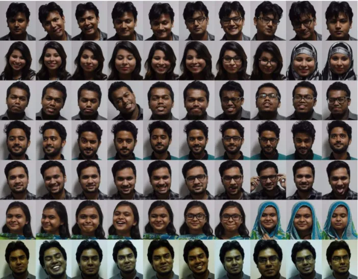
4.7 Database of Face Images:

We have created a database of 231 face images of 21 students and stuffs, each of them have 11 images which taken in both bright light and low light condition. In the database there are male and female student‟s faces, also the skin colors are various types. All the images of individual

21

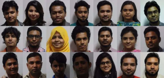
persons are taken with different facial expressions and with or without glasses. There are also two twin brothers face images in the database. The captured size of the images was 5184 x 3456 pixels which were resized and cropped into 180 x 200 pixels. There are two set of databases. First one is Train Database, where all the images are for train the machine. In this database there are 210 images of 21 persons, each one have 10 images with different facial expression. The second database is Test Database, where the captured images are stored. From this database the images first detect face, then resized and cropped into 180 x 200 pixels and then use the normalized image for face recognition.

22

Figure 19: Sample Test Database

4.8 Face Recognition Methodology:

A simple approach to extracting the information contained in an image of a face is to somehow capture the variation in a collection of face images, independent of any judgment of features, and use this information to encode and compare individual face images [7].

In mathematical terms, the principal components of the distribution of faces, or the eigenvectors of the covariance matrix of the set of face images, treating an image as point (or vector) in a very high dimensional space is sought. Each image location contributes more or less to each eigenvector, so that it is possible to display these eigenvectors as a sort of ghostly face image which is called an "eigenface". Eigenfaces can be viewed as a sort of map of the variations between faces. Each individual face can be represented exactly in terms of a linear combination of the eigenfaces. Each face can also be approximated using only the "best" eigenfaces, those that have the largest eigenvalues, and which therefore account for the most variance within the set of face images. The best M eigenfaces span an M-dimensional subspace which we call the "face space" of all possible images [7].

Kirby and Sirovich [7] developed a technique for efficiently representing pictures of faces using principal component analysis. Starting with an ensemble of original face images, they calculated a best coordinate system for image compression, where each coordinate is actually an image that they termed an "eigenpicture". In this research, we have followed the method which was proposed by M. Turk and A. Pentland [9] in order to develop a face recognition system based on the eigenfaces approach. They argued that, if a multitude of face images can be reconstructed by weighted sum of a small collection of characteristic features or eigenpictures, perhaps an efficient way to learn and recognize faces would be to build up the characteristic features by experience over time and recognize particular faces by comparing the feature weights needed to approximately reconstruct them with the weights associated with known individuals.

The basic steps involved in Face Recognition using Eigenfaces Approach are as follows: 1. Acquire initial set of face images known as Training Set (Γi).

2. The average matrix ψ has to be calculated. Then subtract this mean from the original faces (Γi) to calculate the image vector (Փi).

23

∑

Փi = Γi – ψ 3. Find the covariance matrix C by

∑ Փ ՓnT = AAT 4. Compute the eigenvectors and eigenvalues of C.

5. The M‟significant eigenvectors are chosen as those with the largest corresponding eigenvalues 6. Project all the face images into these eigenvectors and form the feature vectors of each face image.

4.9 Training Set of Images:

Let the training set consists of M images representing M image classes. Each of these images can be represented in vector form. Let these images be Γ1; Γ2; … ΓM. The average face of the set is

∑ ………. (1)

Each face image differs from the average face of the distribution, and this distance is calculated by subtracting the average face from each face image. This gives us new image space [7].

Փi = Γi – ψ (i = 1, 2, …, M) ………. (2)

An N x N matrix A is said to have an eigenvector X, and corresponding eigenvalue λ if

AX = λx ………. (3)

Evidently, Eq. (5) can hold only if

det | A – λI | = 0 ………. (4)

Which, if expanded out, is an Nth degree polynomial in λ whose root are the eigenvalues. A matrix is called symmetric if it is equal to its transpose,

A = AT or aij = aji ………. (5)

It is termed orthogonal if its transpose equals its inverse,

AAT = ATA = I ………. (6)

24

AAT = ATA ………. (7) 4.9.1 Theorem:

Eigenvalues of a real symmetric matrix are all real. Contrariwise, the eigenvalues of a real non symmetric matrix may include real values, but may also include pairs of complex conjugate values. The eigenvalues of a normal matrix with non-degenerate eigenvalues are complete and orthogonal, spanning the N dimensional vector space. Let the training set of face images be Γ1; Γ2; … ΓM then the average of the set is defined by

∑ ………. (8)

Each face differs from the average by the vector

Փi = Γi – ψ ………. (9)

An example training set is shown in Figure 18. This set of very large vectors is then subject to principal component analysis, which seeks a set of M ortho-normal vectors, Un which best describes the distribution of the data. The kth vector, Uk is chosen such that

λk ∑ ukTՓn)2 ………. (10)

is a maximum, subject to

ulTuk = δlk = 1, if l = k ………. (11)

= 0, otherwise

The vectors uk and scalars λk are the eigenvectors and eigenvalues, respectively of the covariance matrix

∑ Փ ՓnT = AAT ………. (12)

Where the matrix A = [Փ1, Փ2, … ՓM]. The covariance matrix C, however is N2 x N2 real symmetric matrix, and determining the N2 eigenvectors and eigenvalues is an intractable task for typical image sizes. If the number of data points in the image space is less than the dimension of the space (M < N2, there will be only M-1, rather than N2 meaningful eigenvectors. The remaining eigenvectors will have associated eigenvalues of zero. Consider the eigenvectors vi of AT A such that

AT A Vl = μl vl ………. (13)

Pre multiplying both sides by A, we have

A AT AVl = μl A vl ………. (14)

25

C = A AT………. (15)

Following these analysis, we construct the M x M matrix

L = ATA ………. (16)

Where Lmn = φmT

φn and find the eigenvectors, vl, of L.

These vectors determine linear combinations of the M training set face images to form the eigenfaces ul.

ul ∑ , l = 1, 2, … , M ………. (17)

With this analysis, the calculations are greatly reduced, from the order of the number of pixels in the images (N2) to the order of the number of images in the training set (M) [7].

26

Chapter 5

APPLICATION

5.1 Implementation:

The experiment is implemented over a training set of 210 (21 each of 10 Images). Each image is in RGB level which is normalized to gray level and has dimension of 180 x 200. Each one has 10 images with frontal view with different poses (like frontal view, side view (±45°), closed eyes, smile, blink etc.). In our face database which images we have taken, they are the students and stuffs of BRAC University of Bangladesh. All images are the same size. Some image contains glasses, beard or mustaches in face area. Face images are taken in both bright light and in low light condition. Firstly we construct overall average image. This is the image which is formed by adding all images and dividing by number of images in training set. The eigenvectors of covariance matrix is formed by combining all deviation of training set‟s image from average image. After finding overall average image, we have to find the eigenvectors of the covariance matrix. Since there are 210 images in the training set we need to find 210 eigenvectors that are used to represent our training set.

STEP 1:

A “Create_Database” function Aligns a set of face images from the Training Database (the training set T1, T2,...,TM ). This function reshapes all 2D images of the training database into 1D column vectors. Then, it puts these 1D column vectors in a row to construct 2D matrix 'T'. T is containing all 1D image vectors. Suppose all P images in the training database have the same size of (M x N). So the length of 1D column vectors is MN and 'T' will be a (MN x P) 2D matrix. This function returns the 2D matrix „T‟.

STEP 2:

A “Eigen_Face_Core” function uses Principle Component Analysis (PCA) to determine the most discriminating features between images of faces. This function gets a 2D matrix „T‟, containing all training image vectors and returns 3 outputs which are extracted from training database. It returns 3 values:

m = (MN x 1), Mean of the Training Database A = (MN x P), Matrix of centered image vectors

Eigen_Faces = (MN x (P-1)), Eigen vectors of the covariance matrix of the training database The mean image or the average face image is calculated by

m = (1/P) x sum (Tj's) (j = 1 : P)

Then it calculates the deviation of each image from the mean image. The calculation of the difference image for each image in the training set

27

Ai = Ti – m Then it merges all centered images into A.

We know from linear algebra theory that for a (P x Q) matrix, the maximum number of non-zero eigenvalues that the matrix can have is minimum (P-1, Q-1). Since the number of training images (P) is usually less than the number of pixels (MN), the most non-zero eigenvalues that can be found are equal to P-1. So we can calculate eigenvalues of A' x A (a P x P matrix) instead of A x A' (a MN x MN matrix).

It is clear that the dimensions of A x A' is much larger that A' x A. So the dimensionality will decrease.

L = A' x A; L is the surrogate of covariance matrix C = A x A'.

The Diagonal elements are the eigenvalues for both L = A' x A and C = A x A'.

Then all eigenvalues of matrix L are sorted and those who are less than a specified threshold are eliminated. So the number of non-zero eigenvectors may be less than (P-1).

Eigenvectors of covariance matrix C (or so-called "Eigen_Faces") can be recovered from L‟s Eigenvectors.

Eigen_Faces = A x L‟s Eigenvectors, A is matrix of centered image vectors STEP 3:

A “Face_Recognition” function compares two faces by projecting the images into „facespace‟ and measuring the Euclidean distance between them. Then return the recognized image.

First, it‟s projected centered image vectors into facespace. All centered images are projected by multiplying in Eigen_Face basis‟s vector. Projected vector of each face will be its corresponding feature vector.

Then, it calculates the Euclidean distances between the projected test image and the projection of all centered training images. Test_Image is supposed to have minimum distance with its corresponding image in the training database. The minimum distance with the training image is returned as recognized image.

TRAINING PROCEDURE

Number of images taken for the training procedure

210

Size 180 x 200

Format JPG

Output Minimum Euclidean Distance

Elapsed Time Current Time (for time

calculation)

Recognized image number Detected face image Resized & Cropped image

Recognized image Table 1: Training Procedure

28

5.2 Result Analysis:

The resultant analysis has given below with table and diagram.

FACE DETECTION PROCEDURE

Total number of images taken for the test

231

Number of Detected faces 231

Number of miss detected images 0

Average time elapsed for face detection

0.037416 seconds

Accuracy 100%

Table 2: Face Detection Procedure

FACE RECOGNITION PROCEDURE

Number of images in the Train Database

210 Number of images in the Test

Database

21

Number of recognized images (for manually resized images)

21 Number of misrecognized images

(for manually resized images)

0

Average time elapsed for face recognition

1.163945 seconds

Accuracy 100%

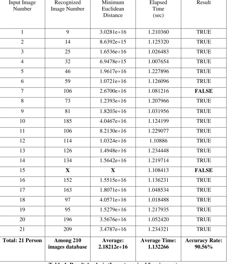
29 Input Image Number Recognized Image Number Minimum Euclidean Distance Elapsed Time (sec) Result 1 9 3.0281e+16 1.210360 TRUE 2 14 8.6392e+15 1.125320 TRUE 3 25 1.6536e+16 1.026483 TRUE 4 32 6.9478e+15 1.007654 TRUE 5 46 1.9617e+16 1.227896 TRUE 6 59 1.0721e+16 1.126096 TRUE 7 106 2.6700e+16 1.081216 FALSE 8 73 1.2393e+16 1.207966 TRUE 9 81 1.8203e+16 1.031956 TRUE 10 185 4.0467e+16 1.124199 TRUE 11 106 8.2130e+16 1.229077 TRUE 12 114 1.0324e+16 1.10886 TRUE 13 126 1.4948e+16 1.234448 TRUE 14 134 1.5642e+16 1.219714 TRUE 15 X X 1.108413 FALSE 16 152 1.5515e+16 1.136231 TRUE 17 163 1.8071e+16 1.048534 TRUE 18 97 4.0571e+16 1.018488 TRUE 19 95 1.5279e+16 1.217935 TRUE 20 196 3.5676e+16 1.052420 TRUE 21 209 3.4787e+16 1.234321 TRUE

Total: 21 Person Among 210 images database Average: 2.18212e+16 Average Time: 1.132266 Accuracy Rate: 90.56%

30

5.3 Face Detection and Recognition Results:

Figure 20: Sample Result 1 (a,b,c)

Figure 21: Sample Result 2 (a,b,c)

31

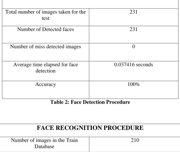
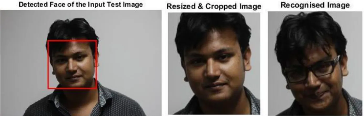
Figure 23: Sample Result 4 (a,b,c) [Twins 1]

Figure 24: Sample Result 5 (a,b,c) [Twins 2]

Figure 25: Sample Result 6 (a,b,c)

32

Chapter 6

FUTURE WORK PLAN

Our future work plan is by using this face detection and recognition system find out a specific person from a crowded place like market place, busy roads, fairs or from a stadium. This can be used to find out a wanted person. In the training database there will be only one person‟s face images with different expression, and the system will captured different images of different people and compare them with the given database. If it finds out similar face it will give an alert.

CONCLUSION

In this paper eigenface based face recognition has been described. The eigenface approach for face recognition process is fast and simple which works well under constrained environment. It is one of the best practical solutions for the problem of face recognition. Eigenfaces method is a principal component analysis approach, where the eigenvectors of the covariance matrix of a small set of characteristic pictures are sought. These eigenvectors are called eigenfaces due to their resemblance of face images. Recognition is performed by obtaining feature vectors from the eigenvectors space.

Many applications which require face recognition do not require perfect identification but just low error rate. So instead of searching large database of faces, it is better to give small set of likely matches. By using Eigenface approach, this small set of likely matches for given images can be easily obtained.

For given set of images, due to high dimensionality of images, the space spanned is very large. But in reality, all these images are closely related and actually span a lower dimensional space. By using eigenface approach, we try to reduce this dimensionality. The lower the dimensionality of this image space, the easier it would be for face recognition. Any new image can be expressed as linear combination of these eigenfaces. This makes it easier to match any two images and thus face recognition.

One of the limitations for eigenface approach is in the treatment of face images with varied facial expressions and with glasses. Also as images may have different illumination conditions. This can be removed by RMS (root mean square) contrast stretching and histogram equalization. In the present work, we used 231 face images as face database. The procedure we used is quite satisfactory. It can recognize both the known and unknown images in the database in various conditions with accuracy 98% to 100% (depend on the database). We think when we use a huge database such as thousand number of images or more, then some misdetection (2%-5%) may happened in the recognition procedure.

33

REFERENCES

[1] Phillip Ian Wilson and Dr. John Fernandez, “Facial Feature Detection Using Haar Classifiers”, Journal of Computing Sciences in Colleges, Volume 21, Issue 4, Pages

127-133, April 2006.

[2] Zhaomin Zhu, Takashi Morimoto, Hidekazu Adachi, Osamu Kiriyama, Tetsushi Koide

and Hans Juergen Mattausch, “Multi-view Face Detection and Recognition Using Haar-like Features”, ResearchGate, January 2004.

[3] M. Gopi Krishna, A. Srinivasulu and Prof (Dr.) T.K.Basak, “Face Detection System on

Ada boost Algorithm Using Haar Classifiers”, International Journal of Modern

Engineering Research (IJMER), Volume 2, Issue.6, Nov-Dec 2012.

[4] Paul Viola and Michael J. Jones, “Robust Real-Time Face Detection”, International Journal of Computer Vision, Volume 57, Issue 2, Pages 137-154, May 2004.

[5] Staffan Reinius, “Object Recognition Using the OpenCV Haar Cascade-classifier on the

iOS Platform”, Uppsala University, Department of Information Technology, 2013.

[6] Pinar Santemiz, Luuk J. Spreeuwers and Raymond N.J. Veldhuis, “Video-based

Side-view Face Recognition for Home Safety”, 33rd WIC Symposium on Information Theory

in the Benelux, Boekelo, the Netherlands, Pages 220-227, 24-25 May 2012.

[7] Dulal Chakraborty, Sanjit Kumar Saha and Md. Al-Amin Bhuiyan, “Face Recognition

using Eigenvector and Principle Component Analysis”, International Journal of

Computer Applications (0975-8887), Volume 50, No.10, July 2012.

[8] B S Venkatesh, S Palanivel and B Yegnanarayana, “Face Detection and Recognition in

an Image Sequence using Eigenedginess”, Indian Conference on Computer Vision,

Graphics and Image Processing, Ahmedabad, India, 2002.

[9] M. Turk and A. Pentland, "Eigenfaces for Recognition", Journal of Cognitive Neuroscience, Volume 3, No.1, Pages 71-86, 1991.

[10] Philipp Wagner, “Face Recognition with GNU Octave/MATLAB”,

34

[11] Anne Hendrikse, Raymond Veldhuis and Luuk Spreeuwers, “Eigenvalue correction

results in face recognition”, 29th Symposium on Information Theory in the Benelux, Leuven, Belgium, Page 27-35, 29-30 May 2008.

[12] Prashant Sharma, Amil Aneja, Amit Kumar and Dr.Shishir Kumar, “Face Recognition using Neural Network and Eigenvalues with Distinct Block Processing”, International Journal of Scientific & Engineering Research, Volume 2, Issue 5, May 2011.

[13] Matthew A. Turk and Alex P. Pentland, “Face Recognition Using Eigenfaces”, Proc. IEEE Conference on Computer Vision and Pattern Recognition: 586–591, 1991.

[14] Matthew A. Turk and Alex P. Pentland, “Eigenfaces for Recognition”, Journal of Cognitive Neuroscience, Volume 3, No.1, Massachusetts Institute of Technology, 1991.

[15] Rajib Saha and Debotosh Bhattacharjee, “Face Recognition Using Eigenfaces”,

International Journal of Emerging Technology and Advanced Engineering, Volume 3, Issue 5, May 2013.

[16] P. N. Belhumeur, J. Hespanha, and D. J. Kriegman, “Eigenfaces vs. Fisherfaces: Recognition using class specific linear projection”, In ECCV (1), 1996.

[17] Kirby, M., and Sirovich, L., "Application of the Karhunen-Loeve procedure for the characterization of human faces", IEEE PAMI, Vol. 12, pp. 103-108, (1990).

[18] Sirovich, L., and Kirby, M., "Low-dimensional procedure for the characterization of human faces", J. Opt. Soc. Am. A, 4, 3, pp. 519-524, (1987).

[19] Kerin, M. A., and Stonham, T. J., "Face recognition using a digital neural network with self-organizing capabilities", Proc. 10th Int. Conf. On Pattern Recognition, pp.738-741, (1990).

[20] Yuille, A. L., Cohen, D. S., and Hallinan, P. W., "Feature extraction from faces using deformable templates", Proc. of CVPR, (1989).