2015
A comparison of QPF from WRF simulations with
operational NAM and GFS output using multiple
verification methods
Haifan Yan Iowa State University
Follow this and additional works at:https://lib.dr.iastate.edu/etd Part of theMeteorology Commons
This Thesis is brought to you for free and open access by the Iowa State University Capstones, Theses and Dissertations at Iowa State University Digital Repository. It has been accepted for inclusion in Graduate Theses and Dissertations by an authorized administrator of Iowa State University Digital Repository. For more information, please [email protected].
Recommended Citation
Yan, Haifan, "A comparison of QPF from WRF simulations with operational NAM and GFS output using multiple verification methods" (2015).Graduate Theses and Dissertations. 14866.
output using multiple verification methods by Haifan Yan
A thesis submitted to the graduate faculty
in partial fulfillment of the requirements for the degree of MASTER OF SCIENCE
Major: Meteorology Program of Study Committee: William A. Gallus, Jr., Major Professor
Xiaoqing Wu Raymond W. Arritt
Iowa State University Ames, Iowa
2015
TABLE OF CONTENTS
ABSTRACT iv
CHAPTER 1 GENERAL INTRODUCTION 1
1.1 Background and Overview
1
1.2 Thesis Organization
3
CHAPTER 2. LITERATURE REVIEW
5
CHAPTER 3. A COMPARISON OF QPF FROM 4 KM GRID
SPACING WRF SIMULATIONS WITH OPERATIONAL NAM AND
GFS OUTPUT USING MULTIFLE VERIFICATION METHODS
8
3.1 Abstract
8
3.2 Introduction
10
3.3 Data and Methodology
13
3.3.1 Model Setup and Data Description
13
3.3.2 Verification Methods
15
3.4 Analysis and Results
19
3.4.1 Climatology Distribution
19
3.4.2 Traditional Verification Methods
20
3.4.3 FSS Analysis
23
3.4.4 MODE
26
a. Intensity Sum
26
b. Location Errors
28
c. Areal Coverage
30
3.5 Conclusions and Discussions
30
3.6 Acknowledgments
33
3.7 References
34
3.8 Tables
37
3.9 Figures
38
CHAPTER 4 ADDITIONAL RESULTS
49
4.1 Introduction
49
4.2 Case Study
50
4.3 River Basins
52
4.4 Figures
54
4.5 Tables
57
CHAPTER 5. GENERAL CONCLUSIONS
58
ACKNOWLEDGMENTS
61
REFERENCES
62
ABSTRACT
The goal for this study was to examine the performance of quantitative precipitation forecasting (QPF) obtained from a high resolution convection-‐allowing model and two coarser resolution operational weather prediction models to better understand any QPF improvements in the convection-‐allowing runs. The ARW-‐WRF model was run over the period from March through November 2013 with 4 km grid spacing to better understand the limits of predictability of short-‐term (12 h) QPF that might be used in hydrology models. WRF runs were performed using NAM and GFS output as the first guess fields in the 3-‐dimensional variational data assimilation system. Radar data were assimilated in WRF runs. Several verification methods were used to compare the QPF from the high-‐resolution runs with coarser operational GFS and NAM QPF. Three traditional grid-‐to-‐grid verification methods, as well as two spatial techniques, neighborhood and object-‐based, were used to verify QPF for 1h, 3h, 6h and 12h precipitation accumulation intervals and two grid configurations.
In general, skill increased more as accumulation interval increased than for spatial scale increasing. At the same neighborhood scale, the grid spacing on which the verifications were done had less impact on the high resolution WRF model than the coarser models. NAM had the worst performance not only for model skill but also for spatial features due to the existence of large dry bias and location errors. Even for some severe floods with large rain coverage, NAM still underpredicted the magnitude of the total rain volume. Moreover, the finer resolution of NAM did not offer any advantages in predicting small-‐scale storms compared to the coarser GFS
model. Both neighborhood and traditional techniques suggested that WRF had much higher skill for larger precipitation thresholds. In addition, WRF had the smallest displacement errors and was able to most correctly forecast the intensity magnitude of simple precipitation objects. The total rain volume obtained from WRF for severe floods is the closest to the observations though WRF still underestimated it. All of the models had the best performance from midnight to early morning, because the least wet bias, location and coverage errors were present then. The lowest skill happened from late morning through afternoon. The major challenge for skill improvement during this period was large displacement errors. The displacement errors started to grow in late morning and reached peak values around late afternoon.
QPF for river basins had higher biases than for the full domain. WRF overpredicted the total rain volume for all river basins and diurnal time periods examined. The skill for the largest basin shared similar characteristics with the full domain, but the smaller basins had much larger discrepancies.
CHAPTER 1. GENERAL INTRODUCTION
1.1 Background and Overview
Numerical weather prediction (NWP) takes current observations of weather to serve as input to the numerical computer models through a process known as data assimilation to produce the future state of weather. Because NWP models are highly nonlinear, a subtle discrepancy in one of hundreds of elements in NWP models such as input lateral conditions, thermodynamic circulations, and physical and chemical processes, may cause the crash of models or produce unpredictable outputs (Cuo et al 2011).
Precipitation is one of the key elements forecast with NWP, as a variety of communities such as agriculture, transportation, airlines, etc, require such information. Moreover, QPF is also the most intractable challenge for NWP because QPF is sensitive to dynamic and thermodynamic processes whose interaction ranges from synoptic scale mechanisms to microscale turbulence (Pereira et al. 1998). Hence, the demands of high resolution and accurate QPF have continued to increase, but QPF still is often poor. The slow improvement of QPF is partly due to the simple treatment of condensation and precipitation processes and also partly due to the underestimates of latent heat release (Zhao and Carr 1996).
Compared with the cold season, warm season QPF is widely known to have low skill, and weather systems during that time are particularly difficult to forecast, because half of warm season precipitation is directly related to meso-‐scale forcing mechanisms, and over 80% of total rainfall is directly or indirectly associated with thunderstorms (Heideman and Fritsch, 1988). Moreover, when storm coverage is
smaller than 10% of the whole domain, QPF will have large displacement discrepancies, and as a result, QPF will lose its skill on small-‐scale high intensity storm cells, which often cause severe flash floods (Johnson and Olsen, 1997). Thus, hydrology forecasters can only use quantitative precipitation estimates (QPE) instead of QPF due to this low skill.
In order to evaluate how poor the model performed and the reasons for the terrible performance, more and more researchers are concerned about the behavior of model verification. Traditional verification methods, such as equitable threat score (ETS; also know as Gilbert skill score), critical success index, odds ratio, probability of detection (PODY) and frequency bias (FBIAS), have been widely used in the past several decades. However, most of the traditional verifications are grid-‐ to-‐grid methods, so they requires near-‐perfect spatial and temporal placement for a forecast to be considered good. Thus, for high-‐resolution models, traditional methods may indicate low skill, so the improvements of numerical models will be hidden by the subtle displacements. In order to better understand the high resolution QPF, a large number of new spatial verification methods have been carried out in recent years.
In this paper, a matrix of verifications including traditional, neighborhood and object-‐based methods will be used to verify the performance of QPF within a convection-‐allowing version of the Weather Research and Forecasting (WRF) model that incorporates radar data assimilation, in order to provide more beneficial information for model developers. Fractions Skill Score (FSS) and Method for Object-‐based Diagnostic Evaluation (MODE), which are recently proposed
neighborhood and object-‐based methods, respectively, will be the two major verifications used in this study to provide a comprehensive scenario about the performance of numerical models over different scales, and for location errors, intensity errors, structure errors, etc. Convection-‐allowing WRF model simulations can help us better understand the spatial and temporal limits of QPF in order to improve QPF for hydrologic use. All the verification methods used in this paper are included in a NWP verification software package developed by Developmental Testbed Center (DTC; http://www.dtcenter.org/), known as Model Evaluation Tools (MET).
The verifications were performed over a long time period during 2013, and covered Iowa and immediately adjacent areas of other states. The QPF of western and northeastern parts of contiguous United States are generally more skillful than central and southeastern regions because of less influence of convective storms in those areas (Sukovich et al 2014). Hence, more information about how QPF skill compares among models in the central United States can assist forecasters and model developers.
1.2 Thesis Organization
This thesis follows the journal paper format. Chapter 1 includes the general introduction to the thesis. Chapter 2 contains a literature review of the studies about QPF improvements and model verifications. Chapter 3 is the paper that will be submitted to Weather and Forecasting. Chapter 4 includes additional results of the study of flood cases and model performance over several river basins. Chapter 5
contains general conclusions from the journal paper and the additional results. The last two chapters are acknowledgments and references separately.
CHAPTER 2. LITERATURE REVIEW
Because QPF skill is still relatively poor, numerous studies have tried to find the limitations of QPF and methods to improve it. However, the formidable challenge in short and medium range QPF is that numerical models are highly nonlinear, so the uncertainties in the models are still poorly understood. It is very difficult to determine which parameter is responsible for a certain deficiency (Fritsch and Heideman, 1989; Cloke and Pappenberger 2009). QPF can be largely influenced by different initializations, microphysics and PBL schemes in the WRF model (Jankov et al. 2007), and the sensitivity of physical schemes depends on initialization data (Jankov et al. 2006).
Many studies have shown that radar data assimilation has a very obvious positive effect on short range (≤12h) QPF (Xiao et al. 2002; Moser et al. 2015). Although model runs with radar assimilation are generally too wet in the first one or two hours (often called hot starts), in general, hot starts have much better performance in intensity, displacement and skill scores than model runs without data assimilation (often called cold starts) (Moser et al. 2015). With higher resolution initializations and data assimilation, the skill of QPF can be improved up to 8-‐9h (Sun et al. 2012). Some studies also try to investigate whether model resolution or interpolation can improve QPF skills. Schwartz et al. (2009) found that although 2km resolution WRF was able to simulate finer structures, but both of the 2km and 4km resolutions had similar convective initiation, evolution and organization. Thus, it is no rush to increase horizontal resolution and ensemble forecasting and post-‐processing should be paid more attention in stead.
The large variety of spatial verification techniques proposed in recent years to evaluate model improvement, Gilliland et al. (2009) summarized the new verification methods into four categories: (i) neighborhood, (ii) scale separation, (iii) object-‐based, and (iv) field deformation. The first two methods both use a spatial filter on one or both of the observation and forecast fields. The last two methods both try to figure out how much the forecast field needs to be corrected in order to achieve meaningful skill. Each type of methods has different advantages to show model performance. Some methods may sensitive to some types of error while some other methods are not (Gilliland et al. 2010). Some methods can both show skill with scales, location errors, intensity errors, structure errors and occurrences, but some methods are not capability to or can only indirectly show some of these feature attributes (Gilliland et al. 2009; 2010). Object-‐based and field deformation can both detect displacement errors and field deformation is the best approach to capture the error of aspect ratio, which will influence the scores from neighborhood and scale separation techniques (Ahijevych et al. 2009).
The FSS, which is one of the neighborhood methods used in this thesis, is dependent on both the neighborhood scales and the spatial rain coverage (Roberts 2008). When the spatial rain coverage is small, many near-‐threshold misses caused by subtle differences can result in large changes in FSS magnitude difference (Mittermaier and Roberts 2009). Thus, it is difficult to have a satisfactory FSS for localized strong convection. FSS is widely used to explore how model skills vary with horizontal resolution. Duc et al. (2013) extended the 2-‐demension spatial FSS to the temporal dimension and demonstrated that temporal resolution is important
for short range QPF at small fuzzy scales. The most remarkable advantage for MODE is that MODE is able to match storm objects in the model field with observed storms. The matching ability is strongly dependent on the object size so the objects of synoptic scale systems can be more predictable, and less simulated objects can not be matched (Davis et al. 2005). Davis et al. (2005) evaluated the performance of WRF using MODE, suggesting that WRF had no large location errors but largely overestimated the size of objects. The overestimation of area reached a maximum in the late afternoon. WRF tends to produce too many rain areas at the scale over 80km and the rain systems are lasting too long (Davis et al. 2005). Numerous studies have used spatial methods as well as traditional techniques for model verifications. Advanced Research version of WRF model (WRF-‐ARW) had a better performance than Nonhydrostatic Mesoscale Model (NMM), but the skill can differ significantly from day to day (Davis et al. 2009).
CHAPTER 3. A COMPARISON OF QPF FROM 4 KM GRID SPACING
WRF SIMULATIONS WITH OPERATIONAL NAM AND GFS OUTPUT
USING MULTIFLE VERIFICATION METHODS
Haifan Yan and William A. Gallus, Jr.
3.1 ABSTRACT
The ARW-‐WRF model was run over 9 months with 4 km grid spacing to better understand the limits of predictability of short-‐term (12 h) quantitative precipitation forecasts (QPF) that might be used in hydrology models. Radar data assimilation was performed to reduce spin-‐up problems that could negatively impact QPF in the first few hours of the simulations. Three traditional grid-‐to-‐grid verification methods, as well as two spatial techniques, neighborhood and object-‐ based, were used to compare the QPF from the high-‐resolution runs with coarser operational GFS and NAM QPF to verify QPF for various precipitation accumulation intervals and the two grid configurations.
In general, NAM had the worst performance not only for model skill but also for spatial features due to the existence of large dry bias and location errors. The finer resolution of NAM did not offer any advantage in predicting small-‐scale storms than the coarser GFS. WRF had a large advantage for high precipitation thresholds. Skill increased more as accumulation interval increased than for spatial scale increasing. At the same neighborhood scale, the high resolution WRF model was less influenced by the grid on which verification was done than the other two models. All
the models had the highest skill from midnight to early morning, because the least wet bias, location and coverage errors were present then. The lowest skill happened from late morning through afternoon. The main barrier for skill improvement during this period was large displacement errors.
3.2 Introduction
Numerical weather prediction (NWP) has been substantially improved over the past decade due to improvements in observation datasets and computation power. Precipitation is one of the key elements forecast with NWP, as a variety of communities such as agriculture, transportation, airlines, etc, require such information. Hence, the demands of high resolution and accurate QPF have continued to increase, but QPF still are often poor.
Warm season QPF is widely known to have low skill as weather systems during that time are particularly difficult to forecast because half of warm season precipitation is directly related to meso-‐scale forcing mechanisms and over 80% of total rainfall is directly or indirectly associated with thunderstorms (Heideman and Fritsch, 1988). Moreover, when storm coverage is smaller than 10% of the whole domain, QPF has been found to have large displacement discrepancies, and as a result, QPF will lose its skill on small-‐scale high intensity storm cells, which can cause severe flash floods (Heideman and Fritsch, 1988). Thus, hydrology forecasters can only use quantitative precipitation estimates (QPE) instead of QPF due to this low skill. Numerous studies have tried to find the limitations of QPF and methods to improve it. However, the essential challenge in short and medium range QPF is that numerical models are highly nonlinear, so the uncertainties of the models are still poorly understood. It is very difficult to determine which parameter is responsible for a certain deficiency (Fritsch and Heideman, 1989; Cloke and Pappenberger 2009). QPF can be largely influenced by different initializations, microphysics and
PBL schemes (Jankov et al. 2007), and the sensitivity of physical schemes depends on initialization data (Jankov et al. 2006).
Many studies have shown that radar data assimilation has a very obvious positive effect on short range (≤12h) QPF (Xiao et al. 2002; Moser et al. 2015). Although model runs with radar assimilation are generally too wet in the first one or two hours (often called hot starts), in general, hot starts have much better performance in intensity, displacement and skill scores than model runs without data assimilation (often called cold starts) (Moser et al. 2015). With higher resolution initializations and data assimilation, the skill of QPF can be improved up to 8-‐9h (Sun et al. 2012).
As grid resolution has been refined, an increasing number of researchers have expressed concern about the verification metrics used to evaluate the performance of these models. Traditional verification methods, such as equitable threat score (ETS; also know as Gilbert skill score), critical success index, odds ratio, probability of detection (PODY) and frequency bias (FBIAS), have been widely used in the past several decades. However, most of the traditional verifications are grid-‐to-‐grid methods, so they are sensitive to small-‐scale errors. Thus, for high-‐resolution models, traditional methods may indicate low skill, so the improvements of numerical models will be hidden by the subtle displacements. In order to better understand high resolution QPF, a large number of new spatial verification methods have been carried out in recent years. Gilliland et al. (2009) summarized the new verification methods into four categories: (i) neighborhood, (ii) scale separation, (iii) object-‐based, and (iv) field deformation. The first two methods both use a
spatial filter on one or both of the observation and forecast fields. The last two methods both try to figure out how much the forecast field needs to be corrected in order to achieve meaningful skill.
In this paper, a matrix of verifications including traditional, neighborhood and object-‐based methods will be used to verify the performance of QPF in a hot start convection-‐allowing model and to compare it with QPF from two operational models in order to provide more beneficial information for model developers. Fractions Skill Score (FSS) and Method for Object-‐based Diagnostic Evaluation (MODE), which are recently proposed neighborhood and object-‐based methods, respectively, will be the two major verification approaches used in this study to provide a comprehensive analysis about the performance of numerical models over different scales, and for location errors, intensity errors, structure errors, etc. Convection-‐allowing WRF-‐ARW model simulations can help us better understand the spatial and temporal limits of QPF in order to improve QPF for hydrologic use. All the verification methods used in this paper are included in a NWP verification software package developed by the Developmental Testbed Center (DTC; http://www.dtcenter.org/), known as Model Evaluation Tools (MET).
The verifications were performed over a long time period during 2013, and covered Iowa and immediately adjacent areas of other states. The QPF of western and northeastern parts of the contiguous United States are generally more skillful than that for the central and southeastern regions because of less influence from small-‐scale convective storms in those areas (Sukovich et al 2014). Hence, more information about how QPF skill compares among models in the central United
States can assist forecasters and model developers. In this paper, section 2 describes model configuration and verification methodology. Section 3 is the analysis of model performance via various verification methods. A discussion and conclusions follow in section 4.
3.3 Data and methodology
3.3.1 Model setup and data description
The ARW-‐WRF version 3.5 (Skamarock et al. 2008) was run every 6 hours (00, 06, 12 and 18 UTC) in order to have a better understanding about the limits of predictability of short-‐term (12h) high resolution QPF that might be used in hydrology models. Both the 12km grid spacing NCEP NAM and 0.5°×0.5° NCEP GFS forecasting output archived from the NOAA National Operational Model Archive and Distribution System (NOMADS) were used as the first guess field in the ARPS three-‐dimensional variational data assimilation (ARPS 3DVAR) system. The ARPS 3DVAR system is part of the Advanced Regional Prediction System (ARPS) which is a regional to storm-‐scale atmospheric modeling system. The ARPS 3DVAR system was used to assimilate into the initial NAM or GFS background fields the corresponding NEXRAD Level II radar data of 9 sites located within the domain region in order to reduce spin up problems normally encountered in model simulations that simply use output from other models for initialization. The 9 sites (Fig. 1) were KABR (Aberdeen, SD), KARX (Lacrosse, WI), KDMX (Des Moines, IA), KDVN (Davenport, IA), KEAX (Kansas City, MO), KFSD
(Sioux Falls, SD), KLSX (St. Louis, MO), KMPX (Minneapolis, MN) and KOAX (Omaha, NE). The input radar data covered the whole simulated domain.
The initial conditions created in the ARPS 3DVAR were then integrated into WRF (hereafter WRF and WRF-‐GFS for NAM and GFS initializations, respectively). The model domain (Fig. 1) was centered at 41.916N and 93.342W with 200×200 horizontal grid points and 4km cell spacing on a Lambert Conformal map projection. The model top pressure was roughly around 60hPa. The physics parameterizations used in this study included the 2-‐moment Thompson microphysics scheme (Thompson et al., 2008), the local MYJ PBL scheme (Janjic, 1994) and the New Goddard longwave and shortwave radiation schemes (Chou and Suarez, 1999).
The two operational models used for WRF initialization, NAM and GFS, were also examined using QPF verification to establish a benchmark to which the WRF runs could be compared. NCEP Stage IV precipitation data were used to represent ground truth in the verification process. The QPF in all of the verified models was interpolated to the same domain configuration as WRF (Hres) through the Unified Postprocessor using the budget method which is able to conserve the more accurate total precipitation magnitude. In addition, in order to study the possible effects of interpolation on various verification metrics, all three models were also interpolated to a lon-‐lat map projection with 0.5°×0.5° GFS (Lres) resolution, which is roughly around 55km. The domain region used for the Lres verification was the portion of the GFS grid for which data were also available from the WRF simulations. Note that since the GFS is a
global model, the 0.5°×0.5° GFS grid has already been regridded, but it is common to use these gridded data for research purposes. Hourly WRF total precipitation output, 3-‐hourly NAM and GFS forecast precipitation data, and hourly and 6-‐hourly STAGE IV data are summed or subtracted into 3h, 6h and 12h accumulation intervals for the verifications performed in the present study.
3.3.2 Verification methods
In this study, five metrics were used to verify the models: ETS, PODY, FBIAS, FSS and MODE. The first three traditional methods were used because they are simple and easy to calculate, and they are also among the most widely used grid-‐to-‐ grid methods. The last two are spatial methods, which will be the focus of verification in this paper. The verification techniques were applied to the precipitation accumulation intervals of 1h, 3h, 6h and 12h.
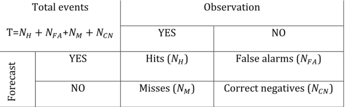
Traditional grid-‐to-‐grid verification methods such as ETS, PODY and FBIAS are calculated based on a contingency table of the form shown in Table 1. Of the total T forecast-‐observation pairs, whether accumulated precipitation (APCP) exceeds a specified threshold is used to define whether a event should fall into hit, false alarm, miss or correct negative category. The ETS is calculated based on the number of counts the events are correctly forecasted to occur to the number of counts they are either forecasted or observed. It is further corrected by the chance forecasts (ref), also widely known as random chance, which is the product of forecasted events and observed events, divided by the total counts. The value of ETS ranges from -‐1/3 to 1. A forecast with no skill will have the value of 0 while a perfect forecast will have the
value of 1. The PODY, which is also called hit rate, represents the fraction of the event occurrences that were forecasted. The FBIAS compares the total number of forecasts and the number of observations. The formulas of ETS, PODY and FBIAS are defined as 𝐸𝑇𝑆 = !!!!"# !!!!!"!!!!!"# (1) 𝑟𝑒𝑓 =(!!!!!")(!!!!!) ! (2) 𝑃𝑂𝐷𝑌= !! !!!!! (3) 𝐹𝐵𝐼𝐴𝑆= !!!!!" !!!!! (4)
where the different subscripts N represent the counts in hits (𝑁!), false
alarms (𝑁!") or misses (𝑁!) category, shown in Table 1. For ETS and PODY, mean values averaged from the 9-‐months of simulations will be shown. However, for FBIAS, it is possible that the count of a forecast event is hundreds of times larger than the number of occurrences which may be a very small value, yielding an enormous FBIAS that would inflate the mean FBIAS in a misleading way. Hence, the counts of events used in the formula above are the total counts of the 9 months rather than the counts of each 3-‐h run. Note that the ETS, PODY and FBIAS are related to each other. Unlike PODY, ETS and FBIAS consider the amount of false alarms. .
The thresholds used to generate binary fields in traditional methods as well as FSS and MODE were 0.254mm (0.01in), 2.54mm (0.1in), 6.35mm (0.25in), and 12.7mm (0.5in), so verifications cover a range from light to relatively heavy intensity.
FSS is a recently proposed neighborhood verification method by Roberts and Lean (2008) and further discussed by Roberts (2008). It is normalized based on Fractions Brier Score (FBS) and is able to show how forecast skill varies with different spatial scales and thresholds. FSS is calculated in the following three steps. First, both forecast (F) and observation (O) fields are transformed into binary fields. A grid box will have the value of 1 if APCP exceeds a specified threshold, otherwise it will have a value of 0. Although APCP is the only variable which will be verified for QPF in this research, other variables such as wind speed and radar reflectivity can also be verified using FSS. Second, the fraction of each grid point (i,j) in the binary observation field O(i,j) (or forecast field F(i,j)) is generated from the neighborhood box centered in (i,j). The fraction (𝑃!! 𝑜𝑟 𝑃!(!)) is calculated by the number of grid
boxes having the value of 1 over the number of all grid boxes within the neighborhood square. Third, FSS is calculated using the following formula:
𝐹𝑆𝑆(!) = 1− 1 𝑁(!) !(!)[𝑃!(!) −𝑃!(!)]! 1 𝑁(!)[ 𝑃!(!) ! + !(!) 𝑃!(!) ! ! ]
where 𝑁(!) is the number of valid neighborhoods at the neighborhood scale of L. The forecasts can be regarded as reasonably skillful when FSS reaches up to 0.5+𝑓! according to Roberts and Lean (2008). The 𝑓! is a sample climatology variable known as base rate (BR), which means the fraction of event occurrences over the whole domain in the binary raw observation field without smoothing; in other words, 𝑓! is the climatological chance of precipitation happening so it is also used to represent random skill. Because FSS is calculated through a fuzzy box, some
displacement errors considered as misses or false alarms in a traditional contingency table can be considered hits as long as the displacement happened within the neighborhood box.
In this study, in order to show how skill varies with scale, an arithmetic sequence of neighborhood sizes, 5, 9, 13 ⋯ 101, was used for smoothing. The largest fuzzy box contained 101×101 pixels, which was around a quarter of the whole domain. Fractions were not calculated if part of a neighborhood box was outside of the domain boundaries.
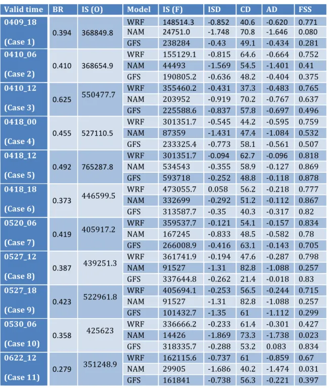
MODE is a newly developed feature-‐based verification methodology based on Davis et al. (2006a,b). Many features of matched pairs between model simulations and observations can be investigated using MODE, such as centroid distance (CD), boundary distance, intensity sum (total rain volume), angle orientation, areal coverage, etc. The raw forecast and observation data are convolved using a cylinder filter with a specified radius. Then the APCP falling within the circular region is averaged to get the convolved field. The filtered regions used for feature comparisons can be obtained after the threshold is applied on the convolved field. The raw data within filtered regions is restored to get simple objects which are individual objects without matching or merging into cluster objects.
In addition to FSS, MODE has a great advantage in directly showing location and structure errors. In correspondence with FSS, the same thresholds were applied to convolved fields to determine the boundaries of filtered regions. Two simple objects of forecast and observation fields were defined as matched pairs only when CD was smaller than 100 grid points. Because a 5-‐grid-‐point radius is almost the
smallest radius that can be used as a practical minimum value according to Davis et al. (2006a) and scale analysis is excluded from the purpose of applying MODE, in order to avoid too much smoothing, this specified radius was applied to generate convolved fields in this study.
Intensity sum (IS) and areal coverage use a normalized formula to link the feature attributes in forecast and observation fields for MODE analysis. The IS difference of the whole domain (ISD) is presented in the following as an example to show the form of normalization:
𝐼𝑆𝐷= 1𝐼𝑆!−𝐼𝑆!
2(𝐼𝑆!+𝐼𝑆!)
where 𝐼𝑆! and 𝐼𝑆! represent the total IS (in mm) over the whole domain in the forecast and observation fields, respectively. Besides the ISD, IS differences for matched pairs (ISDP), areal coverage difference (in grid squares) of the whole domain (AD) and areal coverage difference for matched pairs (ADP) are also normalized using the form of the formula above.
3.4 Analysis and results 3.4.1 Climatology distribution
Before presenting results from various skill metrics, some general rainfall characteristics of the forecasts will be discussed. A climatological frequency distribution of domain averaged 12h accumulated APCP (Fig. 2) suggests that WRF under-‐predicted and NAM over-‐predicted the number of null precipitation cases – these under-‐predicted and over-‐predicted cases have no skill when using FSS. For
flood cases, WRF was the only model able to suggest the true magnitude of heavy rain potential even though it still under-‐predicted the frequency of extreme heavy rainfall cases; NAM and GFS largely underestimated the rainfall amount and greatly underestimated the potential for flash floods. The dry bias of NAM, which might result in low skill at moderate and high thresholds, was the most outstanding issue seen in the climatology.
3.4.2 Traditional verification methods
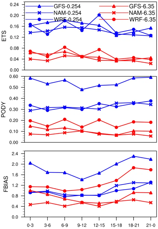
Traditional point-‐to-‐point verification methods are widely used to determine whether simulations can be regarded as “good forecasts”. Although traditional methods are sensitive to subtle displacements and deformations, they are applied on the raw fields without smoothing or convolving, so fewer tunable parameters affect results. In addition, traditional methods can also be used to evaluate the improvements of newly developed verification methods. Hence, ETS, PODY and FBIAS of the three models are shown in Fig. 3 to provide some baseline scores before the application of spatial methods. Because a 3h accumulation interval is the minimum common temporal resolution for the three models, it is the primary accumulation interval that will be used in the following analysis. Diurnal curves in Fig. 3 were performed using a low threshold of 0.254mm and a high threshold of 6.35mm.
The diurnal curves (Fig. 3) not only can directly show model variations with valid time, but also can indirectly show diversification with lead time. The oscillation of ETS for WRF was an indicator of model skill changing with lead time,
because all the peaks occurred during the 0-‐3h and 6-‐9h periods of each simulation, and the periodic low scores occurred in the 3-‐6h and 9-‐12h periods. The skill of hot runs will decrease from a high value during the first three hours and keep decreasing during the 3-‐6h model simulation time and finally will become steady during 6-‐12h according to Moser et al. (2015), resulting in the periodic oscillation evident every 6 hours in the 3-‐h verifications. ETS gave a general score for the whole domain field. Without considering the peak values dominated by data assimilation, WRF did not show large advantages over the two operational models for the light threshold. Because only WRF used radar data assimilation, it was the only model that oscillated with lead time, and the amplitude of the oscillation was smaller for the larger threshold. For GFS at the low threshold, the high value of PODY did not show up in the ETS plot. One possible reason was that GFS had a large number of false alarms.
The skill scores for NAM were not as good as those for GFS, suggesting that the interpolation from the NAM grid to the 4km WRF grid should not be the major reason for the low skill of NAM. However, for GFS, the interpolation to Hres might result in too much smoothing, yielding unreasonably good scores. In general, models had higher ETS and relatively lower PODY during the early morning (6-‐15 UTC) and lower ETS and higher PODY during late afternoon (18-‐00 UTC), indicating that the portion of false alarms became larger from morning to afternoon resulting in the decrease of model skill. This phenomenon was more obvious when comparing PODY and FBIAS. The great variation of FBIAS from late morning to afternoon and the much smoother PODY curves also imply the large fraction of false alarms in the
afternoon because the only difference between FBIAS compared with PODY is the inclusion of false alarms. The much larger FBIAS of GFS at the low threshold was because the interpolation of GFS to a much finer resolution would greatly expand the areas with light precipitation. Meanwhile, the FBIAS reduced to a reasonable magnitude at a larger threshold. Because for light thresholds, there were a large amount of cases that there were no precipitation happening or only a small portion of the domain had rainfall. The interpolation would further enlarge this difference. However, for large thresholds, observed and forecasted precipitation mostly existed at the same time, and also only a much smaller amount of cases contained data over the large thresholds, so the difference between forecasted and observed frequencies can be reduced.
Due to the probability of interpolation effects on model skill scores, ETS, PODY and FBIAS of 3-‐hourly aggregated QPF were also computed on Lres using the threshold of 2.54mm, which is a moderate threshold for 3h QPF. As shown in Fig. 4, when all models were verified on the coarser resolution grid, WRF showed a larger advantage for both ETS and PODY even though GFS was verified on its own grid. This result is likely because the small-‐scale systems simulated by WRF were more realistic than those shown in the coarse resolution operational models. NAM had the lowest skill no matter which configuration was used. In addition, the differences between NAM and the other two models on the same grid were larger in Lres than at the finer resolution. As discussed above, FBIAS includes the fraction of false alarms, unlike PODY, so that the higher PODY of Hres than Lres while having almost the same FBIAS means that false alarms were more common in Lres. With
traditional grid to grid metrics, it is often more difficult for high resolution simulations to reach the same level of accuracy as low resolution model runs because smooth features tend to be rewarded, and fine-‐scale details are penalized if spatial or temporal errors exist. Thus, it makes sense that Lres scores were higher than those of Hres. Thus, verifications will also be performed using the
neighborhood method in order to further check the interpolation effects on model skill scores at the same scale.
3.4.3 FSS analysis
In order to contrast model performance with the increasing of horizontal and temporal scales, the mean FSS, which was aggregated to various accumulation intervals from the whole 12 hour simulation period, is presented in Fig. 5 using different thresholds. Useful skill can be approximated to be 0.5 because of the low mean BR over the 9 months. However, for larger thresholds such as 6.35mm and 12.7mm, almost none of the accumulation intervals and scales were as high as 0.5, and for moderate thresholds such as 2.54mm, only 12 hourly QPF at the scales over 40 grid spacings could reach this useful skill value. Hence, short-‐range QPF for heavy precipitation may still not be skillful enough for hydrology use, and improvements are still needed.
The FSS curves spanning 9 months (Fig. 5) show that, in general, the high resolution WRF model performed better than NAM and GFS, but the GFS interpolated from the coarsest resolution among the three had a better performance than NAM partly due to the dry bias of the NAM. For low and moderate thresholds
such as 0.254mm and 2.54mm, the superiority of WRF was not obvious and the skill of GFS was comparable with WRF for the threshold of 2.54mm and the 12h time accumulation. However, WRF showed an advantage for high thresholds, and the improvements of the scores compared with other models were as large as 0.05-‐0.1. Due to the better performance of GFS, WRF-‐GFS was also evaluated in the experiment in order to check whether a better initialization applied to WRF would improve QPF skill. However, skill scores for WRF-‐GFS did not differ much compared with WRF (not shown here), so these different initializations do not seem to have large effects on the high-‐resolution model QPF of this nine month period making use of radar data assimilation.
WRF showed a larger improvement with the increasing of horizontal scales, suggesting that the main issue for high resolution models is that they are challenged at small scales especially for larger thresholds. Moreover, the improvement of FSS from 5 to 101 fuzzy lengths did not change with longer time accumulations once the period was larger than 1h.. For example, the increase of FSS with scales at a 3h interval was similar to the increase with scales at a 12h interval. In addition, the increase of FSS with increasing spatial scales at the same time interval was smaller than the increase of FSS with increasing time intervals at the same neighborhood size. Thus, for the purpose of increasing simulation QPF skill, an increased accumulation time interval is more important than increased spatial scales because doubling time intervals had a larger skill improvement than doubling neighborhood scales regardless of the model examined.
Because 3h mean FSS failed to meet the threshold for useful skill, an appropriate criterion is needed to select a reasonable neighborhood scale for further analysis. For the threshold of 2.54mm, FSS had a higher rate of increase within 25 smoothing scales though it was also valid for other time intervals and thresholds. Furthermore, at the scale around 25 grid lengths, FSS could reach half of the total FSS augmentation within the neighborhood scales used in this study. Moreover, this neighborhood scale would not cause too much smoothing. Hence, the following QPF skill analysis will use the control scale of 25 grid lengths.
Diurnal cycles of QPF skill are presented in Fig. 6. Verifications were performed on 3 hourly QPF for the threshold of 2.54mm at the smoothing scale of 25 grid lengths. Hourly FSS of WRF was also shown in Fig. 6 in order to provide some detail on variation with lead time. Similar to point-‐to-‐point verifications, NAM and GFS did not show an obvious variation with simulation lead time. The dry bias of NAM existed all day long except for a short period in the afternoon while the wet bias of WRF and GFS existed the entire day except early morning according to the domain averaged APCP (DAP). The lowest skill happened when the rain volume had only small bias errors (late morning, 15-‐18 UTC), so displacement or area/shape errors might be the main cause, which a more detailed study is needed to verify. In the afternoon (18-‐24 UTC), the largest diurnal wet biases were shown by WRF and GFS, which is reasonable because of the preponderance of strong convection, but FSS of GFS and NAM had increased compared to the previous 3 hours. Compared with night and morning, WRF did not lose skill during 18-‐00 UTC as it should due to the variation with lead time indicated by hourly WRF FSS. However, ETS suggested a